Nonequilibrium Anderson model made simple with density functional theory

Abstract

The single-impurity Anderson model is studied within the i-DFT framework, a recently proposed extension of density functional theory (DFT) for the description of electron transport in the steady state. i-DFT is designed to give both the steady current and density at the impurity, and it requires the knowledge of the exchange-correlation (xc) bias and on-site potential (gate). In this work we construct an approximation for both quantities which is accurate in a wide range of temperatures, gates and biases, thus providing a simple and unifying framework to calculate the differential conductance at negligible computational cost in different regimes. Our results mark a substantial advance for DFT and may inform the construction of functionals applicable to other correlated systems.

The description of strongly correlated systems in and, particularly, out of equilibrium is a challenge for any theoretical method. Density functional theory (DFT), despite its many successes in the ab-initio description of atoms, molecules, and solids, is certainly not the first method which comes to mind to tackle strong electronic correlation. In recent years, however, it has been realized that effects of strong correlation may indeed be within reach of the DFT framework CapelleCampo:13 ; LimaSilvaOliveiraCapelle:03 ; MaletGoriGiorgi:12 ; MirtschinkSeidlGoriGiorgi:13 ; MosqueraWasserman:14 ; HodgsonRamsdenChapmanLillystoneGodby:13 ; HodgsonRamsdenGodby:16 ; LorenzanaYingBrosco:12 ; YingBroscoLorenzana:14 ; sf.2008 . For instance, the Kondo plateau in the zero-bias conductance may already be captured at the level of standard Landauer theory combined with DFT Lang:95 ; tgw.2001 ; bmots.2002 provided that an accurate exchange-correlation (xc) potential is used sk.2011 ; blbs.2012 ; tse.2012 . Similarly, it has been shown how the description of Coulomb blockade can be achieved within a DFT framework both in the zero-bias limit ks.2013 ; LiuBurke:15 ; YangPerfettoKurthStefanucciDAgosta as well as at finite bias StefanucciKurth:15 .

The single-impurity Anderson model (SIAM) Anderson:61 is the minimal model for the description of transport through a correlated system. Naturally, it has been studied with a wealth of techniques, especially in recent years. An incomplete list includes the time-dependent density matrix renormalization group HeidrichMeisnerFeiguinDagotto:09 , functional renormalization group (fRG) in the linear KarraschMedenSchoenhammer:10 and non-linear regimes EckelHeidrichJakobsThorwartPletyokhovEgger:10 ; JakobsPletyukhovSchoeller:10 , the numerical renormalization group (NRG) IzumidaSakaiSuzuki:01 ; IzumidaSakai:05 , diagrammatic many-body methods ThygesenRubio:07 ; UimonenKhosraviStanStefanucciKurthLeeuwenGross:11 , and Quantum Monte Carlo (QMC) techniques WernerOkaMillis:09 ; WernerOkaEcksteinMillis:10 . A recent comparative study EckelHeidrichJakobsThorwartPletyokhovEgger:10 shows the level of agreement reached between some of these methods, giving confidence that their results can be considered as accurate reference.

In the present work we exploit state-of-the-art reference values of the nonequilibrium SIAM to construct an accurate DFT functional allowing for the calculation of density and current at negligible computational cost for arbitrary interaction strength. The DFT results are shown to reproduce previously published differential conductances in a wide range of temperatures, on-site potentials and biases with very high accuracy. Our functional does not only provide a fast solution of the nonequilibrium SIAM but also offers an alternative perspective on how to attack more complicated models and/or other physical situations such as, e.g., time-dependent correlated transport.

We work in the i-DFT framework, a recently proposed extension of DFT, designed to study open systems in the steady state StefanucciKurth:15 . i-DFT establishes a one-to-one map between the steady density $n({\bf r})$ of the open system and the steady current $I$ on one hand and the external potential (gate) and bias on the other hand. In the spirit of DFT there exists an open Kohn-Sham (KS) system of non-interacting electrons with the same $n({\bf r})$ and $I$ as the interacting system. In the KS system the Hartree-xc (Hxc) contribution to the gate and the xc contribution to the bias are functionals of $n({\bf r})$ and $I$.

i-DFT for the SIAM – In the SIAM the open system consists of a single-impurity (hence $n$ is the same as the total number of particles $N$) with on-site repulsion $U$ between opposite spin electrons and with energy independent tunneling rate $1/\gamma$ between the impurity and the left/right ($L/R$) electrodes. Denoting by $V$ the external bias, i-DFT leads to two coupled self-consistent KS equations for the steady density $N$ and current $I$ (hereafter $\int\equiv\int\frac{d\omega}{2\pi}$):

$$N=\sum_{\alpha=L,R}\int f\left(\omega+s_{\alpha}\frac{V+V_{\rm xc}}{2}\right)A_{s}(\omega)\;,$$ (1a)

$$I=\frac{\gamma}{2}\sum_{\alpha=L,R}\int f\left(\omega+s_{\alpha}\frac{V+V_{\rm xc}}{2}\right)s_{\alpha}A_{s}(\omega)$$ (1b)

where $s_{R/L}=\pm$ and $f(\omega)=1/(1+e^{\beta(\omega-\mu)})$ is the Fermi function at inverse temperature $\beta=1/T$ and chemical potential $\mu$. Furthermore,

$$A_{s}(\omega)=\frac{\gamma}{(\omega-v_{s})^{2}+\frac{\gamma^{2}}{4}}$$ (2)

is the KS spectral function with KS gate $v_{s}=v+v_{\rm Hxc}$, $v$ being the external gate. Both the Hxc gate $v_{\rm Hxc}=v_{\rm Hxc}[N,I]$ and the xc bias $V_{\rm xc}=V_{\rm xc}[N,I]$ are functionals of the steady density and current, and need to be approximated in practice.

Equations (1b) are the basic self-consistency conditions of the i-DFT approach. They can also be used to derive an expression for the finite-bias differential conductance. The right-hand sides of Eqs. (1b) depend on $V$ both explicitly through the Fermi functions and implicitly through $N$ and $I$ (which enter as arguments of the xc potentials). Differentiation of Eqs. (1b) with respect to $V$ leads to a linear system of coupled equations for $\frac{{\rm d}N}{{\rm d}V}$ and $\frac{{\rm d}I}{{\rm d}V}$ which can easily be solved. Since we are mainly concerned with differential conductances, we only give the explicit solution for this quantity

$$\frac{{\rm d}I}{{\rm d}V}=\frac{1}{D}\left(\frac{G_{-}+G_{+}}{2}+\frac{4}{\gamma}G_{-}G_{+}\frac{\partial v_{\rm Hxc}}{\partial N}\right)$$ (3)

where the denominator is defined as

$$D \equiv 1-\frac{1}{\gamma}(G_{-}-G_{+})\frac{\partial V_{\rm xc}}{\partial N}+\frac{2}{\gamma}(G_{-}+G_{+})\frac{\partial v_{\rm Hxc}}{\partial N}$$ (4)

$$-\frac{1}{2}(G_{-}+G_{+})\frac{\partial V_{\rm xc}}{\partial I}+(G_{-}-G_{+})\frac{\partial v_{\rm Hxc}}{\partial I}$$

$$+\frac{4}{\gamma}G_{-}G_{+}\left(\frac{\partial v_{\rm Hxc}}{\partial I}\frac{\partial V_{\rm xc}}{\partial N}-\frac{\partial v_{\rm Hxc}}{\partial N}\frac{\partial V_{\rm xc}}{\partial I}\right)$$

and

$$G_{\pm}\equiv-\frac{\gamma}{2}\int f^{\prime}\left(\omega\pm\frac{V+V_{\rm xc}}{2}\right)A_{s}(\omega)\;.$$ (5)

For given external gate $v$ and bias $V$, Eq. (3) has to be evaluated at the self-consistent values of $N$ and $I$ found by solving Eqs. (1a) and (1b). Interestingly, at zero bias and arbitrary gate $v$ we have $\frac{\partial v_{\rm Hxc}}{\partial I}|_{I=0}=\frac{\partial V_{\rm xc}}{\partial N}|_{I=0}=0$ and $G_{-}=G_{+}=G_{s}(v)$, where $G_{s}(v)$ is the zero-bias KS conductance. It is straightforward to show that in this case Eq. (3) simplifies to StefanucciKurth:15

$$G(v)\equiv\left.\frac{{\rm d}I}{{\rm d}V}\right|_{V=0}=\frac{G_{s}(v)}{1-G_{s}(v)\left.\frac{\partial V_{\rm xc}}{\partial I}\right|_{I=0}}\;.$$ (6)

Similarly, at the particle-hole (ph) symmetric point $v=-U/2$ (hence $N=1$) and arbitrary bias $V$, we have $\frac{\partial v_{\rm Hxc}}{\partial I}|_{N=1}=\frac{\partial V_{\rm xc}}{\partial N}|_{N=1}=0$. Furthermore, since $v_{\rm Hxc}[1,I]=U/2$ the KS spectral function is even in $\omega$ and therefore $G_{-}=G_{+}=G_{{\rm ph},s}(V)$, where $G_{{\rm ph},s}(V)$ is the finite bias KS conductance at the ph symmetric point. Then Eq. (3) reduces to

$$G_{\rm ph}(V)\equiv\left.\frac{{\rm d}I}{{\rm d}V}\right|_{v=-U/2}=\frac{G_{{\rm ph},s}(V)}{1-G_{{\rm ph},s}(V)\left.\frac{\partial V_{\rm xc}}{\partial I}\right|_{N=1}}\;.$$ (7)

xc potentials at zero temperature – In order to use the i-DFT formulas we need an approximation for $v_{\rm Hxc}$ and $V_{\rm xc}$. In Ref. 20 we showed that the Coulomb blockade diamond is correctly described by the (H)xc potentials

$$\tilde{v}_{\rm Hxc}[N,I] = \frac{U}{4}\sum_{s=\pm}\!\left[1+\frac{2}{\pi}\,{\rm atan}\left(\frac{N+\frac{s}{\gamma}I-1}{\lambda_{1}W_{0}}\right)\right]$$ (8a)

$$\tilde{V}_{\rm xc}[N,I] = -U\sum_{s=\pm}\frac{s}{\pi}\,{\rm atan}\left(\frac{N+\frac{s}{\gamma}I-1}{\lambda_{1}W_{0}}\right)\quad\quad$$ (8b)

where $W_{0}=0.16\gamma/U$ and the fitting parameter $\lambda_{1}$ was chosen to be $\lambda_{1}=1$. The essential property of the (H)xc potentials of Eq. (8) are step-like features occuring at the lines $N\pm I-1=0$ in the $N$-$I$ plane. Unfortunately, these potentials miss the Kondo plateau in $G(v)$ found at zero temperature. In fact, at $T=0$ we have $G=G_{s}$ mera-1 ; mera-2 and the Kondo plateau stems from the KS conductance alone (provided that the exact Hxc gate is used) sk.2011 ; blbs.2012 ; tse.2012 . Although Eq. (8a) at $I=0$ well approximates the exact $v_{\rm Hxc}$ (exhibiting a smeared step of height $U$ at half filling), we see from Eq. (6) that $\frac{\partial V_{\rm xc}}{\partial I}\big{|}_{I=0}$ needs to vanish for the equality $G=G_{s}$ to hold. This is not the case for the approximation in Eq. (8b). To incorporate the Kondo physics in the functionals we have to make sure that (a) the correction to $G_{s}$ vanishes and (b) the Hxc gate at zero current is as accurate as possible. Both requirements can be satisfied with the following ansatz:

$$v_{\rm Hxc}[N,I] = \!\left(1-\tilde{a}^{(0)}[I]\right)\!\tilde{v}_{\rm Hxc}[N,I]+\tilde{a}^{(0)}[I]v_{\rm Hxc}^{(0)}[N]\quad\;\;\;$$ (9a)

$$V_{\rm xc}[N,I] = \!\left(1-\tilde{a}^{(0)}[I]\right)\!\tilde{V}_{\rm xc}[N,I]$$ (9b)

where $v_{\rm Hxc}^{(0)}[N]$ is the parametrization of the $T=0$ Hxc gate of Ref. 15. There are a few constraints which restrict the choice of the function $\tilde{a}^{(0)}$. By symmetry, $\tilde{a}^{(0)}$ should be an even function of the current and, for $\frac{\partial V_{\rm xc}}{\partial I}\big{|}_{I=0}$ to vanish, its value at vanishing current should be unity. Furthermore, the effect of $\tilde{a}^{(0)}$ should fade out as the current increases since the (H)xc potentials of Eq. (8) already give the physically correct picture at finite current. Here we choose the following form satisfying all these conditions

$$\tilde{a}^{(0)}[I]=1-\left[\frac{2}{\pi}\arctan\left(\frac{I}{\gamma W_{0}}\right)\right]^{2}\;.$$ (10)

Equations (9) and (10) completely specify the zero-temperature (H)xc potentials once a value of $\lambda_{1}$ in Eqs. (8) is chosen. In the left panel of Fig. 1 we show that for $\lambda_{1}=2$ the i-DFT $I$-$V$ characteristics at the ph symmetric point is on top of the fRG results EckelHeidrichJakobsThorwartPletyokhovEgger:10 in a wide bias window and for various values of $U/\gamma$. The value $\lambda_{1}=2$ performs well even away from the ph symmetric point, thus supporting the general validity of the functional forms.

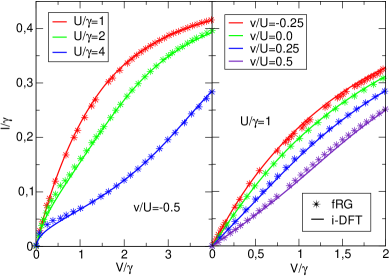
Figure 1: Comparison between fRG and i-DFT $I$-$V$ characterisitcs at zero temperature. Left: at the ph symmetric point $v=-U/2$ for different $U/\gamma$. Right: at fixed $U/\gamma=1$ for different $v/U$. fRG results from Ref. 24.

In the right panel of Fig. 1 we compare the $I$-$V$ characteristics from fRG and i-DFT for various gates at a fixed value of $U/\gamma=1$; the agreement is excellent. We emphasize that in addition to the conceptual simplicity i-DFT is also numerically very efficient: the self-consistent solution of Eqs. (1b) is so fast that the calculation of one $I$-$V$ characteristics requires less than a CPU second.

xc-potentials at finite temperature – We now turn to the construction of the xc potentials at finite temperatures. At the ph symmetric point the zero-bias conductance $G_{\rm ph}(0)$ is known to be a universal function $G_{\rm univ}(T/T_{K})$ of the ratio between $T$ and the Kondo temperature $T_{K}$ AleinerBrouwerGlazman:02 which is given by JakobsPletyukhovSchoeller:10

$$T_{K}=\frac{4}{\pi}\sqrt{U\gamma}\exp\left(-\frac{\pi}{4}\left(\frac{U}{\gamma}-\frac{\gamma}{U}\right)\right).$$ (11)

The function $G_{\rm univ}$ has been calculated using the NRG method in Ref. 35. To reproduce this universal behavior we keep the form in Eqs. (9) except for replacing $W_{0}$ with a temperature dependent $W(T)$ and $\tilde{a}^{(0)}[I]$ with a temperature-dependent functional of $N$ and $I$:

$$a^{(T)}[N,I]=b^{(T)}[N]\tilde{a}^{(T)}[I]\;.$$ (12)

Here $\tilde{a}^{(T)}$ is given by the r.h.s. of Eq. (10) with $W_{0}\to W(T)$ and $b^{(T)}$ is chosen such that $G_{\rm ph}(0)=G_{\rm univ}(T/T_{K})$. The function $W(T)$ (with $W(0)=W_{0}$) accounts for the temperature-dependent broadening of the step-like features of the zero-temperature xc potentials in Eqs. (9). Using Eq. (7) together with our ansatz for the xc bias we obtain the following condition on the function $b^{(T)}$:

$$b^{(T)}[N]=1+\frac{c^{(T)}[N]}{\frac{\partial\tilde{V}_{\rm xc}}{\partial I}\big{|}_{\begin{subarray}{c}N=1\\ I=0\end{subarray}}}\left(\frac{1}{G_{\rm univ}}-\frac{1}{G_{{\rm ph},0}}\right),$$ (13)

where $c^{(T)}[1]=1$ and $G_{{\rm ph},0}\equiv G_{{\rm ph},s}(0)$ is the KS zero-bias conductance at the ph symmetric point. Since $v^{(0)}_{\rm Hxc}[1]=U/2$, from Eqs. (2) and (5) we find $G_{{\rm ph},0}=-\frac{\gamma^{2}}{2}\int f^{\prime}(\omega)/(\omega^{2}+\gamma^{2}/4)$; thus the term in paranthesis is a well defined function of temperature (independent of the functional form of $a^{(T)}$). This construction allows for reproducing with high accuracy the numerical values of $G_{\rm ph}(0)$ of all the reference calculations we compared with.

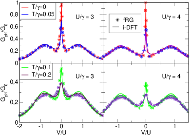
Figure 2: Comparison between fRG and i-DFT differential conductances at the ph symmetric point (in units of the quantum of conductance $G_{0}=1/\pi$) as function of bias $V$ for $U/\gamma=3$ (left) and $U/\gamma=4$ (right). fRG results from Ref. 25.

Although we have not yet specified $c^{(T)}[N]$ for all densities, the property $c^{(T)}[1]=1$ is enough to calculate $G_{\rm ph}(V)$ at finite bias. Aiming to reproduce the results presented in Ref. 25, we found good agreement if we choose the temperature-dependent broadening

$$W(T)=W_{0}\left(1+9\left(\frac{T}{\gamma}\right)^{2}\right)\;.$$ (14)

The dependence on the ratio $T/\gamma$ reflects the physical expectation that broadening is dominated by $\gamma$ at small temperatures and by $T$ at high temperatures. In Fig. 2 we show the differential conductances at the ph symmetric point for $U/\gamma=3$ and $U/\gamma=4$ in a large bias window. In both cases the i-DFT potentials accurately reproduce the fRG results.

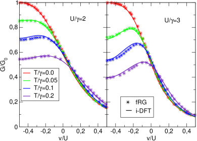
Figure 3: Comparison between fRG and i-DFT zero-bias conductances (in units of $G_{0}=1/\pi$) as function of gate $v$ for $U/\gamma=2$ (left) and $U/\gamma=3$ (right). fRG results from Ref. 25.

We still need an expression for $c^{(T)}$ which, by ph symmetry, is an even function of $(N-1)$. Again good agreement between the i-DFT and fRG finite-temperature zero-bias conductances is found by choosing

$$c^{(T)}[N]=1+\frac{2}{\pi}\delta(T)\arctan\left(\left(\frac{N-1}{\lambda_{2}W(T)}\right)^{2}\right).$$ (15)

As the temperature increases the Kondo plateau in $G(v)$ is suppressed, and this suppression is strongest at the ph symmetric point. The height of the resulting “side peaks” is controlled by

$$\delta(T)=\frac{2}{\pi}\arctan\left(\frac{(U_{c}-U)/\gamma}{\lambda_{2}W(T)}\right)\;,$$ (16)

where the values $\lambda_{2}=3$ and $U_{c}=6\gamma$ best fit the fRG results of Ref. 25. The quality of the i-DFT results for moderate values of $U/\gamma$ can be appreciated in Fig. 3.

Having fixed the parameters $\lambda_{1}$, $\lambda_{2}$ and $U_{c}$ the xc potentials can be used to calculate the differential conductance for any $U/\gamma$ in a wide range of temperature, gate and bias. As a severe test we have analyzed the performance of i-DFT in the very strongly correlated regime. In Fig. 4 we compare the zero-bias conductance of i-DFT and NRG IzumidaSakaiSuzuki:01 ; IzumidaSakai:05 for several temperatures. Once more the agreement is rather satisfactory, only for $U/\gamma=15.91$ and low temperatures the shape of the “side peaks” is slightly different.

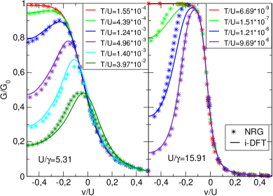
Figure 4: Comparison between NRG and i-DFT zero-bias conductances (in units of $G_{0}=1/\pi$) as function of gate $v$ for $U/\gamma=5.31$ (left) and $U/\gamma=15.91$ (right). NRG results from Ref. 26.

In conclusion, we demonstrated that i-DFT can be used to study the SIAM out of equilibrium, thus disproving the common notion that DFT is not suited for transport through strongly correlated systems. Of course, as the construction of the widely used local density approximation in DFT relies heavily on accurate xc energies of the uniform electron gas (obtained with, e.g., QMC techniques), so the construction of our (H)xc potentials relies heavily on accurate conductances of the SIAM obtained with other methods. However, with an explicit form of the Hxc gate and xc bias the computational problem simplifies enormously since the i-DFT equations describe an effectively non-interacting system. For any temperature, gate, and interaction strength the actual calculation of an $I$-$V$ curve requires only negligible computational effort. With the (H)xc potentials proposed in this work i-DFT becomes a useful and inexpensive method to test and benchmark future theoretical techniques in the SIAM. Furthermore, the ideas behind the construction of the (H)xc potentials are easily transferable to more complicated systems like, e.g., the Constant Interaction Model StefanucciKurth:13 ; ks.2013 ; StefanucciKurth:15 , or to time-dependent transport (through the adiabatic approximation) kskvg.2010 ; Verdozzi:08 ; KarlssonPriviteiraVerdozzi:11 ; HofmannKuemmel:12 ; sds.2013 ; PertsovaStamenovaSanvito:13 ; FuksMaitra:14 and may inform the construction of functionals applicable to ab-initio calculations of correlated materials.

S.K. acknowledges funding by a grant of the ”Ministerio de Economia y Competividad (MINECO)” (FIS2013-43130-P) and by the “Grupos Consolidados UPV/EHU del Gobierno Vasco” (IT578-13). G.S. acknowledges funding by MIUR FIRB Grant No. RBFR12SW0J and EC funding through the RISE Co-ExAN (GA644076).

References

- (1) K. Capelle and V. L. Campo Jr., Phys. Rep. 528, 91 (2013).
- (2) N. A. Lima, M. F. Silva, L. N. Oliveira, and K. Capelle, Phys. Rev. Lett. 90, 146402 (2003).
- (3) F. Malet and P. Gori-Giorgi, Phys. Rev. Lett. 109, 246402 (2012).
- (4) A. Mirtschink, M. Seidl, and P. Gori-Giorgi, Phys. Rev. Lett. 111, 126402 (2013).
- (5) M. A. Mosquera and A. Wasserman, Phys. Rev. A 89, 052506 (2014).
- (6) M. J. P. Hodgson, J. D. Ramsden, J. B. J. Chapman, P. Lillystone, and R. W. Godby, Phys. Rev. B 88, 241102 (2013).
- (7) M. J. P. Hodgson, J. D. Ramsden, and R. W. Godby, Phys. Rev. B 93, 155146 (2016).
- (8) J. Lorenzana, Z.-J. Ying, and V. Brosco, Phys. Rev. B 86, 075131 (2012).
- (9) Z.-J. Ying, V. Brosco, and J. Lorenzana, Phys. Rev. B 89, 205130 (2014).
- (10) P. Schmitteckert and F. Evers, Phys. Rev. Lett. 100, 086401 (2008).
- (11) N. D. Lang, Phys. Rev. B 52, 5335 (1995).
- (12) J. Taylor, H. Guo, and J. Wang, Phys. Rev. B 63, 245407 (2001).
- (13) M. Brandbyge, J.-L. Mozos, P. Ordejón, J. Taylor, and K. Stokbro, Phys. Rev. B 65, 165401 (2002).
- (14) G. Stefanucci and S. Kurth, Phys. Rev. Lett. 107, 216401 (2011).
- (15) J. P. Bergfield, Z.-F. Liu, K. Burke, and C. A. Stafford, Phys. Rev. Lett. 108, 066801 (2012).
- (16) P. Tröster, P. Schmitteckert, and F. Evers, Phys. Rev. B 85, 115409 (2012).
- (17) S. Kurth and G. Stefanucci, Phys. Rev. Lett. 111, 030601 (2013).
- (18) Z.-F. Liu and K. Burke, Phys. Rev. B 91, 245158 (2015).
- (19) K. Yang, E. Perfetto, S. Kurth, G. Stefanucci, and R. D’Agosta, arXiv:1512.07540.
- (20) G. Stefanucci and S. Kurth, Nano Lett. 15, 8020 (2015).
- (21) P. W. Anderson, Phys. Rev. 124, 41 (1961).
- (22) F. Heidrich-Meisner, A. E. Feiguin, and E. Dagotto, Phys. Rev. B 79, 235336 (2009).
- (23) C. Karrasch, V. Meden, and K. Schönhammer, Phys. Rev. B 82, 125114 (2010).
- (24) J. Eckel, F. Heidrich-Meisner, S. G. Jakobs, M. Thorwart, M. Pletyukhov, and R. Egger, New J. Phys. 12, 043042 (2010).
- (25) S. G. Jakobs, M. Pletyukhov, and H. Schoeller, Phys. Rev. B 81, 195109 (2010).
- (26) W. Izumida, O. Sakai, and S. Suzuki, J. Phys. Soc. Jpn. 70, 1045 (2001).
- (27) W. Izumida and O. Sakai, J. Phys. Soc. Jpn. 74, 103 (2005).
- (28) K. S. Thygesen and A. Rubio, J. Chem. Phys. 126, 091101 (2007).
- (29) A.-M. Uimonen, E. Khosravi, A. Stan, G. Stefanucci, S. Kurth, R. van Leeuwen, and E.K.U. Gross, Phys. Rev. B 84, 115103 (2011).
- (30) P. Werner, T. Oka, and A. J. Millis, Phys. Rev. B 79, 035320 (2009).
- (31) P. Werner, T. Oka, M. Eckstein, and A. J. Millis, Phys. Rev. B 81, 035108 (2010).
- (32) H. Mera, K. Kaasbjerg, Y. M. Niquet, and G. Stefanucci, Phys. Rev. B 81, 035110 (2010).
- (33) H. Mera and Y. M. Niquet, Phys. Rev. Lett. 105, 216408 (2010).
- (34) I. Aleiner, P. Brouwer, and L. Glazman, Phys. Rep. 358, 309 (2002).
- (35) T. A. Costi, Phys. Rev. Lett. 85, 1504 (2000).
- (36) S. Kurth and G. Stefanucci, Phys. Status Solidi B 250, 2378 (2013)
- (37) S. Kurth, G. Stefanucci, E. Khosravi, C. Verdozzi, and E. K. U. Gross, Phys. Rev. Lett. 104, 236801 (2010).
- (38) C. Verdozzi, Phys. Rev. Lett. 101, 166401 (2008).
- (39) D. Karlsson, A. Privitera, and C. Verdozzi, Phys. Rev. Lett. 106, 116401 (2011).
- (40) D. Hofmann and S. Kümmel, Phys. Rev. B 86, 201109 (2012).
- (41) P. Schmitteckert, M. Dzierzawa, and P. Schwab, Phys. Chem. Chem. Phys. 15, 5477 (2013).
- (42) A. Pertsova, M. Stamenova, and S. Sanvito, J. Phys.: Cond. Matter 25, 105501 (2013).
- (43) J. I. Fuks and N. T. Maitra, Phys. Rev. A 89, 062502 (2014).