Transformation optics: a time- and frequency-domain analysis of electron-energy loss spectroscopy

Abstract

Electron energy loss spectroscopy (EELS) and Cathodoluminescence (CL) play a pivotal role in many of the cutting edge experiments in plasmonics. EELS and CL experiments are usually supported by numerical simulations, which, whilst accurate, may not provide as much physical insight as analytical calculations do. Fully analytical solutions to EELS and CL systems in plasmonics are rare and difficult to obtain. This paper aims to narrow this gap by introducing a new method based on Transformation optics that allows to calculate the quasi-static frequency and time-domain response of plasmonic particles under electron beam excitation.

Electron energy loss spectroscopy (EELS) has always been at the heart of plasmonics research, playing a major role in the experimental discovery and characterization of plasmons [1, 2, 3]. Experimental and system design progress has been steep since then, now allowing for an energy resolution of a few tens of meV, while maintaining a sub-nanometer spatial resolution [4]. This makes EELS the ideal tool to study plasmons in metallic nano-particles. Particularly, the high spatial resolution and ability to excite the ‘dark’ modes of a nano-particle provide advantages over optical methods. This makes it possible to map out plasmon modes on a sub-nanometer scale and gather information on the local density of states [5, 6], as has been shown in numerous experiments [7, 8, 9, 10, 11, 12]. Quantum effects are negligible in plasmonic systems down to the nanometer scale [13], however for separations between nano-particles less than one nanometer quantum effects become important [14, 15]. Here too, EELS provides an effective method to probe this regime, thanks to its high spatial resolution [14, 16, 13].

Complementing EELS is the method of cathodoluminescence (CL). As in EELS, fast electrons are used in CL to excite plasmons, however, instead of measuring the energy loss experienced by the electrons, CL measures the energy scattered by the nano-particle. This too, gives important insights into the nature of plasmons and has found widespread application in recent experiments [17, 9, 18, 19]. A nice review on both EELS and CL can be found in [20].

On the theoretical side, these experiments are supported by a wide range of numerical methods [13, 21, 22, 23, 24, 25]. Fully analytical methods are rare [20], but have been obtained in the non-retarded limit for geometries for which Poisson’s equation is separable as in, e.g. [26, 27]. This is where Transformation optics (TO) comes in, as it has been shown to be a versatile method in the analytical study of plasmon excitations in nano-particles of more complex shapes [28].

TO is a relatively new tool for the study of Maxwell’s equations that has been developed over the last couple of decades [29, 30, 31, 32]. Early research focused on the design of invisibility cloaks and other functional devices such as beam splitters, beam shifters etc. [33, 34, 35, 36, 37, 38]. In recent years, TO has been applied as an analytical, rather than a design tool and has been used to solve a range of problems in plasmonics [30, 39, 40]. Amongst them, the interaction of closely spaced nano-particles [41], non-locality in plasmonic nano-particles [42] and the calculation of van-der-Waals forces [43, 44]. Most recently, TO has also been used to reveal hidden symmetries in seemingly unsymmetrical structures [45], calculate the optical properties and dispersion relation of plasmonic metal gratings [46], as well as graphene gratings with periodically modulated conductivities [47, 48]. More comprehensive reviews and introductions to TO as used in this paper can be found in [30, 39, 28].

Here we introduce a new application of TO; the analysis of electron energy loss spectroscopy (EELS) problems for plasmonic nano-particles. We will derive analytical expressions for the electron energy loss and photon scattering spectra of a non-concentric annulus and an ellipse (Supplementary Material), calculate the electrostatic potential in frequency space and deduce the time-evolution of the system from this.

Transformation optics for EELS

In a nutshell, TO works by relating two geometries via a coordinate transformation. This is useful if a complicated geometry can be mapped onto a simpler one with higher symmetry, as the higher symmetry often simplifies analytical calculations and makes otherwise intractable problems soluble. In the present case, we consider two-dimensional problems and use conformal transformations [49] to analyze our system. The great advantage of conformal transformations is that they preserve the material properties of the structure, i.e. the in-plane components of the permittivity and permeability tensor are invariant, the electrostatic potential is invariant under these transformations, too [50]. Figure 1 (a) and (b) show examples of systems related via conformal maps (here $z=x+iy$ and $z^{\prime}=x^{\prime}+iy^{\prime}$).

In figure 1 (a) a non-concentric annulus, an ellipse and two nearly touching cylinders can be related to a concentric annulus. These structures have at most two mirror planes, but possess a hidden rotational symmetry evident upon transformation to the concentric annulus [45, 28]. The higher symmetry greatly simplifies calculations of the plasmon eigenmodes of these systems and, as it turns out, also allows us to derive analytical solutions to these systems if an electron moves past. The non-concentric annulus is analyzed in the main body of the paper, the ellipse is given in the Supplementary Materials and results for the cylindrical dimers are published elsewhere together with an analysis of two nearly touching spheres [51]. We would like to mention to the reader that we have developed an open-source GUI software package implementing the TO calculations for the three two-dimensional cases, calculating electron energy loss and scattering spectra. It is available from the authors.

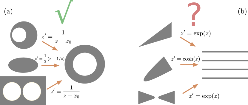
Figure 1: Schematics of conformal transformations between related systems. Figure (a) shows a set of different geometries, for which a transformation optics analysis of EELS calculations is possible. The ellipse is studied in the supplemental material and results for the dimer are published elsewhere. Figure (b) shows some proposed structures for future applications of the TO approach to EELS calculations.

Figure 1 (b) shows another set of geometries, a sharp knife-edge, a hyperbolic knife and a bow-tie antenna with blunt tips, which can all be related to a system of periodic slabs [52, 53]. These structures have also been previously analyzed with TO, so we feel confident that EELS calculations for these structures can be tackled with TO. We do not provide an analysis of them here, but would like to highlight the generality of the approach.

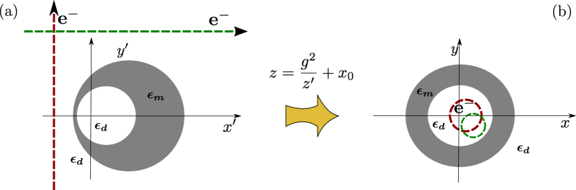
Figure 2: Schematics of conformal transformations between related systems. Figure (a) shows the system under investigation in this paper. It can be related to the concentric annulus shown in (b). The simple geometry of the annulus allows for an analytical solution of the problem.

The remainder of this paper focuses on the non-concentric annulus. A more detailed view of the problem considered here is shown in figure 2. It shows the relation between the non-concentric annulus frame (physical frame) and concentric annulus (virtual frame). We consider a (line) electron moving past the non-concentric annulus in the vertical (red line) and horizontal direction (green line). Since charge is a conserved quantity, the transformation automatically gives us the electron’s trajectory in the virtual frame. There the electron moves on a closed circular trajectory, however, it does so with a non-uniform speed. This makes it difficult to calculate the electrostatic potential of the electron in the virtual frame. In the physical frame the electrostatic potential of the moving electron is very simple to calculate, since the electron moves on a straight line with constant velocity. We will thus adopt a hybrid approach here. We will first calculate the source potential of the electron in the original, physical frame, then transform it to the virtual frame. We then calculate the response of the metal nano-particle in the virtual frame of the concentric annulus and finally transform the electrostatic potential back to the physical frame.

A word of caution is needed here. The calculation presented below is strictly in 2-D, this means the moving electron really is a line electron and all results are per unit length. In reality, the electron is a point particle, so when it moves past the nano-particle it not only loses momentum/energy in the in-plane direction, but also in the out-of plane direction. This is not captured by the 2-D calculation, however there is a workaround. The trick is to filter out the electrons which have not lost any momentum out-of plane. Those effectively behave as line charges.

The electrostatic potential of an electron moving in a straight line in the vertical direction at position $x_{e}^{\prime}$ is easily deduced as

$$\phi^{sou}= -\frac{\lambda}{4\pi\epsilon_{0}\omega}e^{-i\frac{\omega}{v}y^{\prime}}e^{-|x^{\prime}-x^{\prime}_{e}|\frac{\omega}{v}}.$$ (1)

Here $c_{e}$ is the (line) electron’s velocity, $\lambda$ is the charge per unit length and both $\omega$ and $c_{e}$ are positive. If the electron passes to the left of the non-concentric annulus, the potential at the surface of the non-concentric annulus can be written as

$$\phi^{sou}= \frac{\lambda\exp\left[\frac{\omega}{c_{e}}x_{e}\right]}{4\pi\epsilon_{0}\omega}\exp\left[-\frac{\omega}{c_{e}}(z^{\prime})^{*}\right],$$ (2)

since $x_{e}^{\prime}<x^{\prime}$. The potential in the virtual frame is obtained by substituting coordinates

$$\phi^{sou}= \frac{\lambda\exp\left[\frac{\omega}{c_{e}}x_{e}\right]}{4\pi\epsilon_{0}\omega}\exp\left[-\frac{\omega}{c_{e}}\left(\frac{g^{2}}{z-x_{0}}\right)^{*}\right]$$ (3)

$$= \frac{\lambda\exp\left[\frac{\omega}{c_{e}}x_{e}\right]}{4\pi\epsilon_{0}\omega}\exp\left[-\frac{\omega}{c_{e}}\left(\frac{g^{2}}{re^{i\phi}-x_{0}}\right)^{*}\right],$$ (4)

which can be expanded into the eigenfunctions of the concentric annulus [51]

$$\phi^{sou}= \sum_{n=0}^{\infty}a_{n}^{s\pm}\left(\frac{r}{x_{0}}\right)^{\pm n}e^{\mp in\phi}.$$ (5)

Expressions for the expansion coefficients can be found in the Supplementary Material.

The form of the source potential suggests that the total electrostatic potential in the virtual frame can be written as

$$\phi_{I} =\sum_{n=0}^{\infty}\left[a_{n}^{s+}e^{-in\phi}+(b_{n}+a_{n}^{rad})e^{in\phi}\right]\left(\frac{r}{x_{0}}\right)^{n}\quad \mbox{for}\quad r<x_{0}$$ (6)

$$\phi_{II} =\sum_{n=0}^{\infty}\left[(a_{n}^{s-}+a_{n}^{rad})\left(\frac{x_{0}}{r}\right)^{n}e^{in\phi}+b_{n}\left(\frac{r}{x_{0}}\right)^{n}e^{in\phi}\right] \mbox{for}\quad R_{0}>r>x_{0}$$ (7)

$$\phi_{III} =\sum_{n=0}^{\infty}\left[c_{n}\left(\frac{x_{0}}{r}\right)^{n}e^{in\phi}+d_{n}e^{in\phi}\left(\frac{r}{x_{0}}\right)^{n}\right] \mbox{for}\quad R_{1}>r>R_{0}$$ (8)

$$\phi_{IV} =\sum_{n=0}^{\infty}e_{n}e^{in\phi}\left(\frac{x_{0}}{r}\right)^{n} \mbox{for}\quad R_{1}>r,$$ (9)

where $R_{0}$ and $R_{1}$ are the inner and outer radius of the annulus, respectively. The coefficients $b_{n},c_{n},d_{n}$ and $e_{n}$ are the usual electrostatic scattering coefficients and can be determined by demanding continuity of the tangential component of the electric field and normal component of the displacement field at the interfaces. The coefficients $a_{n}^{rad}$ are not present in a purely electrostatic calculation; they encode information about the radiative reaction of the system and have to be determined from an additional ‘radiative’ boundary condition [46, 51]. Details can be found in the supplementary. Using this additional boundary condition all scattering coefficients can be uniquely determined.

Spectra for non-concentric annulus

Energy is a conserved quantity. This means the energy absorbed by the annulus in the virtual frame is the same as the energy absorbed by the non-concentric annulus in the physical frame and similarly for the power scattered by the nano-particles.

The power absorbed by the annulus can be deduced from the resistive losses in the metal, i.e. from

$$Q= \frac{1}{2}\int_{S}dS\mbox{Re}(\mathbf{j}^{*}\cdot\mathbf{E}),$$ (10)

with the integration area $S$ corresponding to the area of the annulus. As the electrostatic potential is known, formulas for the electric fields and currents are easily deduced and the integration readily carried out (see Supplementary Material). After a straightforward calculation the power absorbed by the annulus and hence also by the non-concentric annulus is obtained as,

$$Q= \pi\omega\epsilon_{0}\mbox{Im}(\epsilon_{m})\sum_{n=0}^{\infty}\left[n|c_{n}|^{2}x_{0}^{2n}(R_{0}^{-2n}-R_{1}^{-2n})+n|d_{n}|^{2}x_{0}^{-2n}(R_{1}^{2n}-R_{0}^{2n})\right].$$ (11)

The power scattered by the nano-particles can also be calculated analytically. It can be obtained by imagining that the non-concentric annulus is surrounded by a fictional absorber far away from the boundary of the non-concentric annulus. One can then imagine that the power scattered by the nano-particle is going to be equal to the power absorbed by the fictional absorber. In the annulus frame this fictional absorber corresponds to a point particle at position $x_{0}$ with non-zero polarizability. The power scattered is then simply equal to the power absorbed by the fictional point particle. Details on this approach can be found in [54] and the Supplementary Material. Carrying out the detailed calculation one arrives at the following formula for the power scattered by the non-concentric annulus

$$P_{sca}= \frac{\pi^{2}\epsilon_{0}k_{0}^{2}g^{4}\omega}{2}\left|\sum_{n}\frac{nb_{n}}{x_{0}}\right|^{2}.$$ (12)

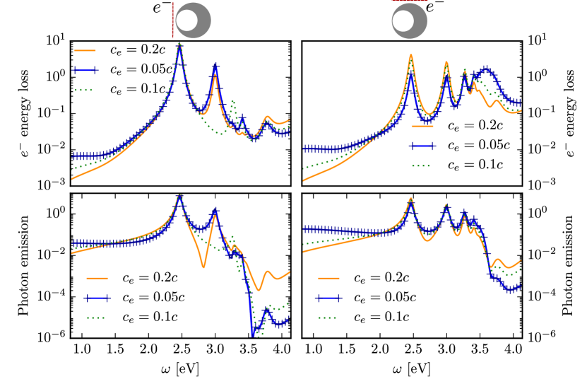
Figure 3: Electron energy loss (top) and photon emission spectra (bottom) for an electron passing to the left (left) and electron passing along the top (right). The electron energy loss spectra give the energy loss probability density for the exciting electron. It is in units of [eV^-1 per electron per unit length]. The photon emission spectra give the photon emission probability density in units of [eV^-1 per electron per unit length]. Both curves are normalized such that the area under the curve is unity. The total energy lost by the electron and the total energy scattered over all frequencies is given in table 1 for all the cases shown here. The geometrical parameters were set to $g^{2}=2\times 10^{-8}$, $x_{0}=1.5$, $R_{0}=\exp(1)$ and $R_{1}=\exp(1.2)$. This gives a diameter of $\approx 21nm$ for the outer cylinder and $\approx 15nm$ for the diameter of the inner cylinder of the non-concentric annulus. The thickness at the thinnest point is $\approx 0.6nm$. The distance of the electron to the particle was $\approx 3.3nm$.

It is well known that moving electrons can probe both bright and dark modes of plasmonic nano-particles (this is also one major advantage over far field light excitation of plasmons). Eq.11 and Eq.12 are in accordance with this statement, as they contain contributions from all plasmon modes of the system.

In EELS and cathodoluminescence experiments measurable quantities are the total electron energy loss, i.e. the amount of energy an electron passing the nano-particle loses and the photon scattering spectrum, i.e. the amount of energy the nano-particle scatters. The total electron energy loss is obtained by adding the power absorbed and power scattered by the nano-particle. The photon scattering spectrum is often given in terms of photon number emission spectrum, i.e. the number of photons emitted at a particular frequency. In this case the expression in Eq. 12 has to be divided by $\hbar\omega$ to convert an energy to a photon number.

Figure 3 gives both electron energy loss spectra and photon emission spectra for an electron passing the non-concentric annulus vertically and horizontally. Both spectra are given as loss probability density and photon emission probability density, i.e. the area under the curves is unity. The total energy lost by the electron and total energy scattered by the nano-particle is given in table 1.

	Vertical		Horizontal
	$e^{-}_{loss}$ $[eVm^{-1}]$	$N(\gamma)$	$e^{-}_{loss}$ $[eVm^{-1}]$	$N(\gamma)$
$c_{e}=0.05c$	$6.05\times 10^{-11}$	$3.76\times 10^{-12}$	$3.05\times 10^{-11}$	$8.71\times 10^{-13}$
$c_{e}=0.1c$	$8.62\times 10^{-11}$	$5.69\times 10^{-12}$	$7.56\times 10^{-11}$	$3.63\times 10^{-12}$
$c_{e}=0.2c$	$6.55\times 10^{-11}$	$4.15\times 10^{-12}$	$6.97\times 10^{-11}$	$3.65\times 10^{-12}$

Table 1: Table giving the total energy loss defined by $\int e_{loss}^{-}(\omega)d\omega$ in units of [eV per unit length] and the total number of photons emitted $N(\gamma)$. The different rows are for different electron velocities, the first two columns are for a (line) electron moving past the particle in the vertical direction and the last two columns are for a (line) electron moving horizontally past the particle. The geometrical parameters were set to $g^{2}=2\times 10^{-8}$, $x_{0}=1.5$, $R_{0}=\exp(1)$ and $R_{1}=\exp(1.2)$, giving a particle of diamater $\approx 21nm$. The distance of the electron to the particle was $\approx 3.3nm$.

In figure 3 we consider an electron passing the non-concentric annulus vertically (left) and horizontally (right). We used experimental data for the permittivity of silver for the non-concentric annulus [55]. The different curves correspond to different electron velocities $c_{e}=0.05c,0.1c,0.2c$ with corresponding kinetic energies of $\approx 0.64eV,2.57eV,10.54eV$.

The intuitive picture of what is happening is this. The electron moves past the nano-particle very rapidly, transferring energy to the particle over a very short window of time. The faster the electron, the smaller this time window. Heisenberg’s uncertainty principle $t_{\Delta}\omega_{\Delta}\approx\hbar$ then lets us estimate the spread of frequencies over which excitations will happen (a few $eV$ in this case). The faster the electron, the larger the range of frequencies present, meaning that we would expect faster electrons to be better suited to excite higher frequency modes. A conclusion which is supported by the source potential in Eq.1, which decays much faster for slower velocities or higher frequencies. This is not what is observed. In the energy loss spectrum of the vertical case the loss probability for the mode at $\omega\approx 3.5$ is larger for the electrons with $c_{e}=0.05$ and $c_{e}=0.1c$ than for the fastest electrons. But this is not a universal behavior as the first mode at $\omega\approx 2.4eV$ is excited similarly for all three speeds, whereas the mode at $\omega=2.5$ is entirely absent for the electron with velocity $c_{e}=0.1c$. The results indicate that not all modes of the system might be observable with electrons of arbitrary velocity.

The reason for the vanishing of this mode is an ‘accidental degeneracy’. While the formulae for the resistive losses and scattering spectrum run over all modes of the system, they are all proportional to the expansion coefficients of the source, $a_{n}^{s-}$. These are damped oscillating functions with respect to the parameter $\omega/c_{e}$. For the quadrupole mode at $\omega\approx 2.5eV$ the zero of the expansion coefficient $a_{2}^{s-}$ coincides with the resonance frequency of this particular mode. Hence, the mode is not present in the exciting source potential and it remains dark.

This accidental degeneracy does not have to be a nuisance, since it allows the ‘switching off’ of a particular mode by tuning the energy of the exciting electrons. For example, switching off the mode at $\omega\approx 2.5eV$ for the electron with $c_{e}=0.1c$ resulted in a much stronger excitation of the next order mode at $\omega\approx 3.2$, which is barely visible for the slower and faster electron. In the horizontal case this is not as easily achieved, as the expansion coefficients have both real and complex components, which means it is harder to tune them to vanish at the same time in the relevant frequency range. This explains why the spectra for the electrons moving horizontally vary much more smoothly with respect to different electron velocities. The other difference between the horizontal and vertical case is that the higher order modes near the surface plasma frequency are excited much more efficiently when the electrons move past the nano-particle in the horizontal direction.

The photon emission spectra show similar behavior for the even modes below the surface plasma frequency, but drop sharply (in both cases) for the odd modes above the surface plasma frequency, as would be expected.

Time-Response of non-concentric annulus

The great advantage of the TO approach to EELS calculations is that analytical expressions for the electrostatic potential $\phi(x^{\prime},y^{\prime},\omega)$ can be derived and easily computed. The time-evolution of these systems can thus be efficiently reconstructed from the frequency domain via a fourier transform

$$\phi(x^{\prime},y^{\prime},t) =\int_{-\infty}^{\infty}d\omega\phi(x^{\prime},y^{\prime}\omega)e^{-i\omega t}$$ (13)

$$=2\mbox{Re}\left[\int_{0}^{\infty}d\omega\phi(x^{\prime},y^{\prime}\omega)e^{-i\omega t}\right].$$ (14)

Here we used the reality condition on the potential $\phi(-\omega)=\phi^{*}(\omega)$ [56]. These calculations are fast enough to be carried out on a state-of-the-art laptop within a couple of seconds (or minutes depending on the number of spatial points), which makes it possible to create videos of the time-evolution of these systems. See supplementary files. For the time-evolution analysis we used a Drude model, $\epsilon_{m}=1-\omega_{p}^{2}/(\omega(\omega+i\gamma))$, with $\gamma=0.32eV$ and $\omega_{p}=8$ for the permittivity of the nano-particle and assumed the surrounding dielectric was air with $\epsilon_{d}=1$.

An electron moving past a nano-particle excites many modes at once. The number of excited modes and there relative strength can be inferred from the energy electron loss spectrum. The different spectra for electrons passing the particle in the vertical and horizontal direction indicate that the time response for the vertical case will be dominated by the first two (dipole and quadrupole) modes, while the one for the horizontally moving electron is expected to be more complicated with contributions from higher order modes as well. This is exactly what can be observed in the videos provided as supplementary materials. They show the time evolution of the vertical and horizontal electric field components as the electron moves past the nano-particle. While the electric field pattern observed for the vertical case only shows one or two oscillations of the electric field as one moves around the particle, the pattern for the horizontal case is much more complicated and shows many nodes and anti-nodes, indicating that higher order modes are contributing significantly to the scattered and induced fields.

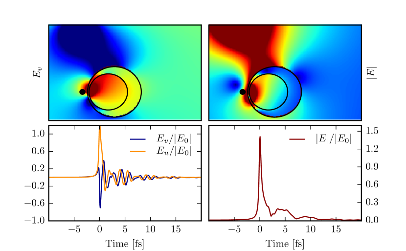
Figure 4: The top panel shows the electric field distribution at a specific time point (indicated by the arrow). $E_{v}$ on the left and $|E|$ on the right. The bottom panel shows the time response of the crescent at a particular point (marked by the black dot in the top panel). In this case the electron moves vertically to the left of the nano-particle. The plots in the bottom panel have been normalised by the maximum source field at the particular point. The geometrical parameters were set to $g^{2}=2\times 10^{-8}$, $x_{0}=1.5$, $R_{0}=\exp(1)$ and $R_{1}=\exp(1.2)$, giving a particle of diamater $\approx 21nm$. The distance of the electron to the particle was $\approx 3.3nm$.

Singular nano-crescents have been shown to efficiently harvest light and concentrate it at their singular point. This focusing of the energy into a small area can also be observed here. For the electron passing horizontally modes are excited at the ‘fat’ end of the non-concentric annulus, but can then be seen to propagate towards the thinnest point, squeezing the energy into a tiny area. Unlike the singular crescent, where the fields never reach the singularity, they can travel past this point in the non-concentric annulus and travel on a circle until all the energy is lost through scattering or resistive losses [40, 28].

Figure 4 and 5 give snapshots of the video. The upper panels show contour plots of the electric fields at a particular point in time, while the lower ones give the time-evolution of the fields at a particular point in space. The fields in the time-evolutions graphs have been normalized by the maximum source field at that particular point. $t=0$ has been chosen as the point in time when the electron moves through $x^{\prime}=0$ (horizontal case) and $y^{\prime}=0$ (vertical case). As expected the time-evolution looks more complicated for the horizontal case, with many more oscillations in the fields than for the vertically passing electron. It should also be noted that the response in the vertical case is much more sudden, both in excitation and decay.

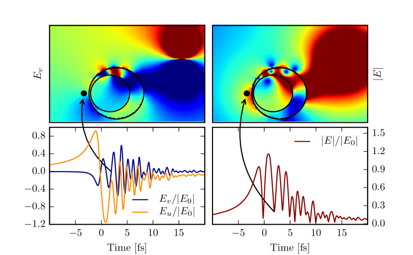
Figure 5: The top panel shows the electric field distribution at a specific time point (indicated by the arrow). $E_{v}$ on the left and $|E|$ on the right. The bottom panel shows the time response of the crescent at a particular point (marked by the black dot in the top panel). In this case the electron moves horizontally along the top of the nano-particle. The plots in the bottom panel have been normalised by the maximum source field at the particular point. The geometrical parameters were set to $g^{2}=2\times 10^{-8}$, $x_{0}=1.5$, $R_{0}=\exp(1)$ and $R_{1}=\exp(1.2)$, giving a particle of diamater $\approx 21nm$. The distance of the electron to the particle was $\approx 3.3nm$.

Conclusion

In this paper, we introduced a new approach based on Transformation optics to calculate the frequency and time-domain response of plasmonic systems under electron beam excitation. Transformation optics previously proved to be a valuable tool in the analysis of the mode spectra and optical response of plasmonic particle of complex geometries. Here, we showed that it can also be employed to calculate the electron energy loss and photon scattering spectra of plasmonic nano-particles under electron beam excitation, with very good agreement between analytics numerical simulations (see Supplementary Material). Moreover, due to the analytical nature of this approach, it has been possible to obtain the time-domain response of the nano-particle in a very time-efficient manner by Fourier transforming the frequency domain solution. We believe that Transformation optics is very well suited to analyze EELS and CL systems in plasmonics and will give additional physical insight into these.

References

- [1] R. H. Ritchie. Plasma Losses by Fast Electrons in Thin Films. Phys. Rev., 106(5):874–881, 1957.
- [2] Hiroshi Watanabe. Experimental evidence for the collective nature of the characteristic energy loss of electrons in solids - Studies on the dispersion relation of plasma frequency. Journal of the Physical Society of Japan, 11(2):112–119, 1956.
- [3] C. J. Powell and J. B. Swan. Origin of the characteristic electron energy losses in aluminum. Physical Review, 115(4):869–875, 1959.
- [4] Ondrej L Krivanek, Jonathan P Ursin, Neil J Bacon, George J Corbin, Niklas Dellby, Petr Hrncirik, Matthew F Murfitt, Christopher S Own, and Zoltan S Szilagyi. High-energy-resolution monochromator for aberration-corrected scanning transmission electron microscopy/electron energy-loss spectroscopy. Philosophical transactions. Series A, Mathematical, physical, and engineering sciences, 367(1903):3683–3697, 2009.
- [5] F. J. García De Abajo and M. Kociak. Probing the photonic local density of states with electron energy loss spectroscopy. Physical Review Letters, 100(10):1–4, 2008.
- [6] Ulrich Hohenester, Harald Ditlbacher, and Joachim R. Krenn. Electron-energy-loss spectra of plasmonic nanoparticles. Physical Review Letters, 103(10):1–4, 2009.
- [7] Jaysen Nelayah, Mathieu Kociak, Odile Stéphan, F. Javier García de Abajo, Marcel Tencé, Luc Henrard, Dario Taverna, Isabel Pastoriza-Santos, Luis M. Liz-Marzán, and Christian Colliex. Mapping surface plasmons on a single metallic nanoparticle. Nature Physics, 3(5):348–353, 2007.
- [8] Olivia Nicoletti, Martijn Wubs, N. Asger Mortensen, Wilfried Sigle, Peter a. van Aken, and Paul a. Midgley. Surface plasmon modes of a single silver nanorod: an electron energy loss study. Opt. Express, 19(16):15371, 2011.
- [9] R. Gómez-Medina, N. Yamamoto, M. Nakano, and F. J García De Abajo. Mapping plasmons in nanoantennas via cathodoluminescence. New Journal of Physics, 10:105009, 2008.
- [10] Pratik Chaturvedi, Keng H Hsu, Anil Kumar, Kin Hung Fung, James C Mabon, and Nicholas X Fang. Imaging of Plasmonic Modes of Silver Nanoparticles Using High-Resolution. ACS Nano, 3(10):2965–2974, 2009.
- [11] Ai Leen Koh, Kui Bao, Imran Khan, W. Ewen Smith, Gerald Kothleitner, Peter Nordlander, Stefan A. Maier, and David W. Mccomb. Electron energy-loss spectroscopy (EELS) of surface plasmons in single silver nanoparticles and dimers: Influence of beam damage and mapping of dark modes. ACS Nano, 3(10):3015–3022, 2009.
- [12] Ai Leen Koh, A Fernandez-Dominguez, S Maier, J Yang, and D McComb. Mapping of Electron-Beam-Excited Plasmon Modes in Lithographically-Defined Gold Nanostructures. Nano Lett., 11:1323–1330, 2011.
- [13] Huigao Duan, Antonio Fernandez, Michel Bosman, Stefan a Maier, and Joel K W Yang. Nanoplasmonics : Classical down to the Nanometer Scale Nanoplasmonics : Classical down to the Nanometer Scale. Nano Letters, 2012.
- [14] Jonathan a Scholl, Aitzol García-Etxarri, Ai Leen Koh, and Jennifer a Dionne. Observation of quantum tunneling between two plasmonic nanoparticles. Nano Lett., 13(2):564–9, 2013.
- [15] Kevin J Savage, Matthew M Hawkeye, Rubén Esteban, Andrei G Borisov, Javier Aizpurua, and Jeremy J Baumberg. Revealing the quantum regime in tunnelling plasmonics. Nature, 491(7425):574–577, 2012.
- [16] Jonathan a. Scholl, Ai Leen Koh, and Jennifer a. Dionne. Quantum plasmon resonances of individual metallic nanoparticles. Nature, 483(7390):421–427, 2012.
- [17] M. Kuttge, E. J R Vesseur, and A. Polman. Fabry-Perot resonators for surface plasmon polaritons probed by cathodoluminescence. Applied Physics Letters, 94(18):29–32, 2009.
- [18] Toon Coenen and Albert Polman. Polarization-sensitive cathodoluminescence Fourier microscopy. Optics Express, 20(17):18679, 2012.
- [19] Ashwin C. Atre, Benjamin J. M. Brenny, Toon Coenen, Aitzol García-Etxarri, Albert Polman, and Jennifer a. Dionne. Nanoscale optical tomography with cathodoluminescence spectroscopy. Nature Nanotechnology, 10(5):429–436, 2015.
- [20] F. J. García De Abajo. Optical excitations in electron microscopy. Reviews of Modern Physics, 82(1):209–275, 2010.
- [21] Yang Cao, Alejandro Manjavacas, Nicolas Large, and Peter Nordlander. Electron Energy-Loss Spectroscopy Calculation in Finite-Difference Time-Domain Package. ACS Photonics, 2(3):369–375, 2015.
- [22] Christian Matyssek, Jens Niegemann, Wolfram Hergert, and Kurt Busch. Computing electron energy loss spectra with the Discontinuous Galerkin Time-Domain method. Photonics and Nanostructures - Fundamentals and Applications, 9(4):367–373, 2011.
- [23] Nahid Talebi, Wilfried Sigle, Ralf Vogelgesang, and Peter van Aken. Numerical simulations of interference effects in photon-assisted electron energy-loss spectroscopy. New Journal of Physics, 15(5):053013, 2013.
- [24] Nicholas W. Bigelow, Alex Vaschillo, Vighter Iberi, Jon P. Camden, and David J. Masiello. Characterization of the electron- and photon-driven plasmonic excitations of metal nanorods. ACS Nano, 6(8):7497–7504, 2012.
- [25] F. J. García de Abajo and A. Howie. Retarded field calculation of electron energy loss in inhomogeneous dielectrics. Physical Review B, 65(11):115418, 2002.
- [26] B.L. Illman, V.E. Anderson, R.J. Warmack, and T.L. Ferrell. Spectrum of surface-mode contributions to the differential energy-loss probability for electrons passing by a spheroid. Physical Review B, 38(5):3045–3049, 1989.
- [27] N. Zabala, A. Rivacoba, and P. Echenique. Coupling effects in the excitations by an external electron beam near close particles. Physical Review B, 56(12):7623–7635, 1997.
- [28] A. Aubry and J. B. Pendry. Active Plasmonics and Tuneable Plasmonic Metamaterials, chapter 4, pages 105–152. John Wiley & Sons, Inc., 2013.
- [29] A. J. Ward and J. B. Pendry. Refraction and geometry in maxwell’s equations. J. Mod. Opt., 43(4):773–793, 1996.
- [30] J. B. Pendry, A. Aubry, D. R. Smith, and S. A. Maier. Transformation optics and subwavelength control of light. Science, 337(6094):549–552, 2012.
- [31] H. Y. Chen, C. T. Chan, and Sheng P. Transformation optics and metamaterials. Nat. Mater., 9(5):387–AC396, 2010.
- [32] U. Leonhardt and T. G. Philbin. Transformation optics and the geometry of light. Prog. Opt., 53:69–152, 2009.
- [33] J. B. Pendry, D. Schurig, and D. R. Smith. Controlling electromagnetic fields. Science, 312(5781):1780–1782, 2006.
- [34] Ulf Leonhardt. Optical conformal mapping. Science, 312(5781):1777–1780, 2006.
- [35] Marco Rahm, Steven A. Cummer, David Schurig, John B. Pendry, and David R. Smith. Optical design of reflectionless complex media by finite embedded coordinate transformations. Phys. Rev. Lett., 100:063903, Feb 2008.
- [36] Do-Hoon Kwon and Douglas H. Werner. Polarization splitter and polarization rotator designs based on transformation optics. Opt. Express, 16(23):18731–18738, Nov 2008.
- [37] Paloma a Huidobro, Maxim L Nesterov, Luis Martín-Moreno, and Francisco J García-Vidal. Transformation optics for plasmonics. Nano letters, 10(6):1985–90, June 2010.
- [38] Yongmin Liu, Thomas Zentgraf, Guy Bartal, and Xiang Zhang. Transformational plasmon optics. Nano letters, 10(6):1991–7, June 2010.
- [39] J. B. Pendry, Yu Luo, and Rongkuo Zhao. Transforming the optical landscape. Science, 348(6234):521–524, 2015.
- [40] J. Zhang and A. V. Zayats. Multiple fano resonances in single-layer nonconcentric core-shell nanostructures. Opt. Express, 21(7):8426–8436, 2013.
- [41] A. Aubry, D. Y. Lei, S. A. Maier, and J. B. Pendry. Interaction between plasmonic nanoparticles revisited with transformation optics. Phys. Rev. Lett., 105(23):233901, 2010.
- [42] A. I. Fernández-Domínguez, A. Wiener, F. J. García-Vidal, S. A. Maier, and J. B. Pendry. Transformation-optics description of nonlocal effects in plasmonic nanostructures. Phys. Rev. Lett., 108:106802, 2012.
- [43] J. B Pendry, A. I. Fernandez-Dominguez, Y. Luo, and R. Zhao. Capturing photons with transformation optics. Nature Physics, 9(8):518–522, 2013.
- [44] Y. Luo, R. Zhao, and J. B. Pendry. van der waals interactions at the nanoscale: the effects of non-locality. Proc. Natl. Acad. Sci. U.S.A., 111:18422, Dec 2014.
- [45] Matthias Kraft, J. B. Pendry, S. A. Maier, and Yu Luo. Transformation optics and hidden symmetries. Phys. Rev. B, 89:245125, Jun 2014.
- [46] Matthias Kraft, Yu Luo, S. A. Maier, and J. B. Pendry. Designing plasmonic gratings with transformation optics. Physical Review X, 5(3):1–9, 2015.
- [47] P A Huidobro, M Kraft, R Kun, S A Maier, and J B Pendry. Graphene, plasmons and transformation optics. Journal of Optics, 18(4):044024, 2016.
- [48] Paloma A. Huidobro, Matthias Kraft, Stefan A. Maier, and John B. Pendry. Graphene as a tunable anisotropic or isotropic plasmonic metasurface. ACS Nano, 10(5):5499–5506, 2016.
- [49] Ablowitz Mark J. and Fokas A. S. Complex variables: introduction and applications, volume Cambridge texts in applied mathematics. Cambridge University Press, 2003.
- [50] Y. Luo. Transformation optics applied to plasmonics. Dissertation of doctoral degree, Imperial College London, London, 2012.
- [51] Yu Luo, Matthias Kraft, and J.B. Pendry. Harnessing transformation optics for understanding electron energy loss and cathodoluminescence. submitted to PNAS, May 2016.
- [52] Y. Luo, J. B. Pendry, and A. Aubry. Surface plasmons and singularities. Nano Lett., 10(10):4186–4191, 2010.
- [53] V. Pacheco-Pena, M. Beruete, A.I. Fernandez-Dominguez, Y. Luo, and M. Navarro-Cia. Conformal transformation for nanoantennas. In Meta ’15 New York - USA Proceedings, 6th International Conference on Metamaterials, Photonic Crystals and Plasmonics, META’15, New York, USA, Aug. 2015.
- [54] A. Aubry, D. Lei, S. A. Maier, and J. B. Pendry. Conformal transformation applied to plasmonics beyond the quasistatic limit. Phys. Rev. B, 82:205109, Nov 2010.
- [55] P. B. Johnson and R. W. Christy. Optical constants of the noble metals. Phys. Rev. B, 6(12):4370–4379, 1972.
- [56] John D. Jackson. Classical Electrodynamics. Wiley, third edition, August 1998.