Labyrinthine water flow across multilayer graphene-based membranes: molecular dynamics versus continuum predictions

Abstract

In this paper we investigate the hydrodynamic permeance of water through graphene-based membranes, inspired by recent experimental findings on graphene-oxide membranes. We consider the flow across multiple graphene layers having nanoslits in a staggered alignment, with an inter-layer distance ranging from sub-nanometer to a few nanometers. We compare results for the permeability obtained by means of molecular dynamics simulations to continuum predictions obtained by using the lattice Boltzmann calculations and hydrodynamic modelization. This highlights that, in spite of extreme confinement, the permeability across the graphene-based membrane is quantitatively predicted on the basis of a continuum expression, taking properly into account entrance and slippage effects of the confined water flow. Our predictions refute the breakdown of hydrodynamics at small scales in these membrane systems. They constitute a benchmark to which we compare published experimental data.

I Introduction

Recent progress in chemical modification and conversion technology concerning graphene sheets has opened up the possibility of producing a bulk carbon material having a molecular-scale porous structure with well-controlled pores and inter-layer distances, as represented by the graphene oxide (GO) membrane. Dikin et al. (2007); Novoselov et al. (2012); Joshi et al. (2015); Yoon, Cho, and Park (2016) In contrast to the graphite, in which the graphene sheets are held together by van der Waals forces with the distance around $3.4$ Å and there is no space for fluid molecules, the inter-layer distance in GO membrane is maintained typically at $\sim 1$ nm, i.e., a few times larger than fluid molecules, and it works as a membrane for fluids flowing through the gap between the layers. The inter-layer distance may be systematically tuned in the range of sub-nanometers up to $10$ nm. Yang et al. (2013) Such graphene-based materials have attracted significant attentions as multi-functional membranes that exhibit peculiar transport phenomena relevant to nano-scale flows. Qiu et al. (2011); Nair et al. (2012); Sun et al. (2013); Cheng and Li (2013); Huang et al. (2013); Huang, Ying, and Peng (2014); Park and Jung (2014); Aghigh et al. (2015); Hegab and Zou (2015); Cheng et al. (2016); Cruz-Silva, Endo, and Terrones (2016); Koltonow and Huang (2016) In Ref. Nair et al., 2012, a GO film fabricated to have pores (or slits) was shown to allow high-speed water flow across the film, whereas it was almost completely impermeable to any other liquids or gases. The GO film in Ref. Huang et al., 2013, which was designed to have channels of $3-5$ nm in width, was shown to permeate water very efficiently. More recently, ion transports through nanoslits in stacking multiple graphene sheets have been examined and the phenomena specific to the complex geometries have been reported. Cheng et al. (2016)

Since the inter-layer distance ranges from a few to tens of the size of fluid molecules, the transport phenomena unique to multi-layered graphene membranes observed experimentally are often attributed to atomic-scale effects that can not be addressed in the continuum theory. However, a systematic investigation of the flow across such complex porous structure, which lies at the edge between the atomic scale and the continuum framework, is still lacking. In particular, it is still difficult to clarify whether the peculiar transport phenomena observed experimentally are indeed dominated by the breakdown of hydrodynamics, the specific geometrical complexity of a small-scale structure, or caused by other effects such as the surface chemistry of the modified graphene. Boukhvalov, Katsnelson, and Son (2013); Wei, Peng, and Xu (2014); Ban et al. (2016)

In the present study, we investigate the water flow across a multi-layered graphene with arrays of staggered nanoslits using the molecular dynamic (MD) simulation, and develop a corresponding continuum model for comparison, in order to clarify the applicability of classical hydrodynamics and to benchmark its predictions. Focusing on the influence of the geometry, we assume that the layers consist of pure graphene sheets without chemical modification, but the width of the nanoslits and the inter-layer distance are controllable from several angstroms to a few nanometers, mimicking the porous structure of GO membranes. Nair et al. (2012); Xia et al. (2015); Hu and Mi (2013); Ban et al. (2016); Akbari et al. (2016) Here, we measure the water flux across the membrane and make systematic comparison with the permeance predicted by the developed continuum model. Good agreement is obtained if the model parameters are chosen appropriately, the values of which are discussed by analyzing basic problems such as an independent nanoslit and a flow through two parallel graphene sheets.

II Geometrical set-up and MD simulations

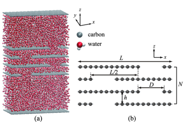
Figure 1: (a) A snapshot of the system. (b) Geometrical parameters characterizing the multi-layered graphene membrane.

We consider a physical model of multi-layered graphene membrane as depicted in Fig. 1, where graphene sheets having nanoslits of width $D$ are laminated in the $z$ direction. The nanoslits are arranged in a staggered fashion such that the displacement in the $x$ direction is $L/2$, and the common inter-layer distance is $h$. The membrane is sandwiched by two water reservoirs, and each of the two ends is closed by a graphene sheet with no slit. The graphene sheet at the ends plays the role of a piston controlling the pressure in the reservoir. The periodic boundary condition is assumed in the $x$ and $y$ directions. The system is considered as a pseudo two-dimensional problem (Fig. 1(b)), as treated in Refs. Nair et al., 2012; Joshi et al., 2014. The porous structure of the membrane is characterized by the four geometrical parameters, namely, the periodicity $L$ in the $x$ direction, the width $D$ of the nanoslit, the inter-layer distance $h$, and the number of graphene layers $N$. Here, it is emphasized that $D$ and $h$ are defined as distances between the centers of carbon atoms (in contrast with the continuum model discussed in Sec. III).

In the MD simulation, the interaction potential employed for water molecules is the TIP4P model. Jorgensen et al. (1983) The water-graphene interaction potential is determined by the Lorentz–Berthelot mixing rule, Allen and Tildesley (1989); Hansen and McDonald (2006) employing the Lenard–Jones (LJ) parameters of AMBER96 for carbon atoms. Cornell et al. (1995) The contact angle of a water droplet on a pure graphene sheet is $66^{\circ}$, which we evaluated using the method described in Ref. Werder et al., 2003, and thus the surface of the graphene in the present study is hydrophilic.

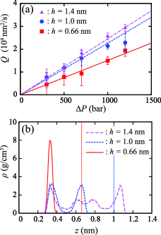
Figure 2: (a) Volumetric flux $Q$ per unit length in the $y$ direction versus applied pressure difference $\Delta P$. The geometrical parameters are $D=0.99$ nm, $L=6.82$ nm, and $N=2$. The cases of $h=0.66$, $1.0$, and $1.4$ nm are shown in the figure. The error bar indicates the standard deviation for the data measured at every $1$ ps (see also the main text). The linear fit for each $h$ is also indicated by the lines. (b) The cross-sectional density distribution of water between two graphene layers. The origin of the $z$ coordinate is the position of one graphene layer, and the positions of the other graphene layer for the cases of $h=0.66$ and $1.0$ nm are indicated by the dotted line.

The MD simulations are implemented using the open-source code LAMMPS. LAM The number of molecules and the size of the simulation box are fixed during each simulation, while the temperature is maintained at $300$ K using the Nosé–Hoover thermostat (NVT ensemble). The time integration is carried out with the time step $1$ fs, and SHAKE algorithm is employed to maintain the water molecules as rigid. Ryckaert, Ciccotti, and Berendsen (1977) The LJ interactions are treated using the standard method with spherical cutoff of $9.8$ Å, while the long-range Coulomb interactions are treated using the particle-particle particle-mesh (PPPM) method. The non-periodicity in the $z$ direction is dealt with by applying the periodic boundary condition with empty spaces outside the pistons, and the artifacts from the image charges due to periodic conditions in the $z$ direction are removed by using the method in Ref. Yeh and Berkowitz, 1999.

The pressure in the reservoirs is controlled by tuning the force acting on the pistons. More precisely, the atoms of the pistons are constrained such that they move only in the $z$ direction, and the force on all atoms is tuned so that the force per unit surface corresponds to the desired pressure.

The water permeance is evaluated by measuring the fluxes induced by the pressure difference $\Delta P$ between the reservoirs. Before running each simulation with the pressure difference, the system is equilibrated for $0.5$ ns with maintaining the pressures of both reservoirs at $1$ bar ($10^{5}$ Pa). The size of the simulation box is $1.97\sim 3.94$ nm in the $y$ direction, and the initial height of the reservoirs in the $z$ direction is more than $3.5$ nm. In Fig. 1(a), the length in the $y$ direction is $3.94$ nm, and the geometrical parameters are $L=6.82$ nm, $D=1.42$ nm, $h=1$ nm, and $N=4$. The number of molecules contained in this case is $8640$.

Figure 2(a) plots the volumetric flux $Q$ as a function of $\Delta P$ in the cases of $h=0.66$, $1.0$, and $1.4$ nm with $D=0.99$ nm, $L=6.82$ nm, and $N=2$. The volumetric flux is obtained from the linear fit of the motion of piston $z_{p}(t)$. The time-series values of $z_{p}(t)$ averaged over $1$ ps at every $1$ ps are used for the linear fit, and the standard deviation is shown by the error bar in the figure. Although the error bar is large for the small values of $\Delta P$, the measured flux is found to increase linearly with $\Delta P$, and the water permeance ${\cal L}_{\rm hyd}=Q/\Delta P$ is obtained independent of $\Delta P$ in the range considered here.

The water density between two graphene sheets during the production runs for Fig. 2(a) is shown in Fig. 2(b). The density distribution along the $z$ axis at the midpoint of the two nanoslits staggered in the $x$ direction is plotted, for the case of $\Delta P=1000$ bar. The excluded volume near the carbon atoms in the graphene is clearly observed, which should be properly taken into account in the continuum model. The consistency of this density profile with the model parameter describing this excluded volume will be shown in Sec. IV.1 in the course of determination of the parameters contained in the continuum model.

In Fig. 3, we show the MD results for the permeance as a function of the inter-layer distance. Since the flux $Q$ increases linearly with $\Delta P$ as shown in Fig. 2, the permeance is evaluated for at least four values of $\Delta P$ in the range $\Delta P\leq 1200$ bar and the averaged value is plotted. The standard deviation for different values of $\Delta P$ is shown by the error bars in the figure. The geometrical parameters are $L=6.82$ nm, $N=2$, and $D=0.99$ nm in Fig. 3(a) or $D=1.42$ nm in Fig. 3(b). Since the diameter of a water molecule is about $3$ Å, the width of the nanoslit is twice as large as a water molecule in Fig. 3(a), and three times in Fig. 3(b), taking into account the excluded volume near the carbon atoms (cf. Fig. 2(b)). The model equations plotted by the lines will be derived in the following section, and the MD results in comparison with the model predictions will be discussed in Sec. IV.

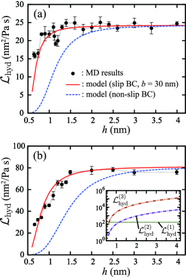
Figure 3: Two-dimensional hydrodynamic permeance ${\cal L}_{\rm hyd}$ versus the inter-layer distance $h$ obtained by means of the MD simulations. The solid and dashed lines are the prediction of the continuum model in Eq. (4), with respectively a slip length of $b=30$ nm and no-slip boundary conditions, see Sec. III. The geometrical parameters are $L=6.82$ nm, $N=2$ and $D=0.99$ nm in panel (a) or $D=1.41$ nm in panel (b). The error bar indicates the standard deviation for the data obtained for different values of the pressure differences $\Delta P$. The inset of panel (b) shows the contributions of decomposed permeances defined in Sec. III, in the case of $b=30$ nm.

III Continuum model of hydrodynamic permeance

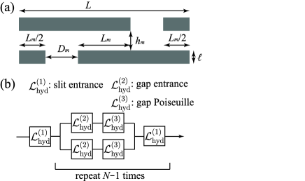
Figure 4: (a) Coarse-grained geometry of the membrane. (b) Continuum model of water permeance.

In this section, we develop a model based on continuum hydrodynamics in order to predict the flow through the membrane in Fig. 1. To this end, we define a two-dimensional channel depicted in Fig. 4(a), as a coarse-grained model for the original porous structure of carbon atoms. The definition of the width of the slit $D_{m}$ and the inter-layer distance $h_{m}$ differs from the molecular parameters $D$ and $h$ defined in Fig. 1(b) in terms of the distance between carbon atoms, due to the exclusion of water molecules close to the graphene surfaces (see Fig. 2(b)). At this stage, we introduce exclusion distances for the slit width and inter-layer distance, defined as $\delta D=D-D_{m}$ and $\delta h=h-h_{m}$, respectively.

The model is built by decomposing the flow from the entrance to the exit of the membrane into three parts. First, the permeance describing the flow resistance at the entrance of a nanoslit is written as: Hasimoto (1958)

$${\cal L}_{\rm hyd}^{(1)}=\dfrac{\pi D_{m}^{2}}{32\eta},$$ (1)

where $\eta$ is the viscosity of water. This is the two-dimensional version of the Sampson formula for the flow through a single circular pore in an infinitely thin wall. Sampson (1891) Note that this is a hydrodynamic permeance per unit length in the $y$ direction (with unit m${}^{2}/$Pa s).

The effect at the entrance into the gap $h_{m}$ between the layers is described by essentially the same formula as Eq. (1). A slight modification is necessary, however, because there is only one edge at this entrance, and the other side is in contact with the plane surface. We consider this situation as the half of the entrance of width $2h_{m}$, which results in:

$${\cal L}_{\rm hyd}^{(2)}=\dfrac{1}{2}\dfrac{\pi(2h_{m})^{2}}{32\eta}.$$ (2)

Finally, the permeance of the flow through the gap $h_{m}$ of length $L_{m}$ is given by the formula for the plane Poiseuille flow with Navier’s slip boundary condition:

$${\cal L}_{\rm hyd}^{(3)}=\dfrac{h_{m}^{3}}{12\eta L_{m}}+\dfrac{bh_{m}^{2}}{2\eta L_{m}},$$ (3)

where the second term on the right-hand side arises from the slip boundary condition with $b$ being the slip length.

The hydrodynamic permeance of the whole membrane is obtained by combining ${\cal L}_{\rm hyd}^{(1)}\sim{\cal L}_{\rm hyd}^{(3)}$ as in Fig. 4(b). Since the permeances in series are combined through the harmonic mean while those in parallel are simply added, the complete model is expressed as:

$${\cal L}_{\rm hyd}=\left[\dfrac{N}{{\cal L}_{\rm hyd}^{(1)}}+(N-1)\left(\dfrac{{\cal L}_{\rm hyd}^{(2)}+{\cal L}_{\rm hyd}^{(3)}}{2{\cal L}_{\rm hyd}^{(2)}{\cal L}_{\rm hyd}^{(3)}}\right)\right]^{-1}.$$ (4)

In order to verify the accuracy of Eq. (4) at this stage within the continuum description, we carry out a direct numerical analysis of the Navier–Stokes equations for the geometry in Fig. 4(a). We employ the lattice Boltzmann method (LBM) Chen and Doolen (1998); Succi (2001) as the numerical method, the detailed algorithm of which is described in Ref. Yoshida and Hayashi, 2014. The no-slip boundary condition is implemented using the standard halfway bounce-back rule, and the perfect-slip condition is realized with the specular reflection. At a boundary sufficiently far form the membrane in the $z$ direction, a pressure difference of $\Delta P=1$ bar is imposed using the method in Ref. Zou and He, 1997. The hydrodynamic permeance ${\cal L}_{\rm hyd}$ is then evaluated by measuring the flux $Q$ in the $z$ direction.

The hydrodynamic permeance ${\cal L}_{\rm hyd}$ predicted by the LBM is plotted as a function of $h_{m}$ in Fig. 5. The geometrical parameters used in the LBM are $D_{m}=1$ nm, $L_{m}=3.7$ nm, $\ell=0.31$ nm and $N=2$ in Fig. 5(a) or $N=3$ in Fig. 5(b). The results of Eq. (4) with $b=0$ (no-slip), $0.2$ and $b=1$ nm are also shown in the figure. The permeance of the perfect-slip case shown in the figure is obtained by taking the limit of $b\to\infty$ in Eq. (4):

$${\cal L}_{\rm hyd}=\left(\dfrac{N}{{\cal L}_{\rm hyd}^{(1)}}+\dfrac{N-1}{2{\cal L}_{\rm hyd}^{(2)}}\right)^{-1}.$$ (5)

In the model equations, the same values of the geometrical parameters as those in the LBM are used. Note furthermore that for completeness, the dissipation across the thickness $\ell$ of the slit could be accounted for. A crude approximation consists in using a Poiseuille like dissipation, with a permeance given as $D_{m}^{3}(1+6b/D_{m})/(12\eta\ell)$. This is actually a small correction as compared to ${\cal L}_{\rm hyd}$ in Eq. (4), but using a value $\ell=0.2$ nm allows to reach perfect agreement with numerical LBM results, as shown in Fig. 5. As a further remark, we quote that the perfect-slip case ($b\to\infty$, i.e. $b\gg D_{m},\,h_{m}$) does not contain $\ell$, so that no parameter is tuned. It is clear form the figure that the model in Eqs. (4) reproduces the LBM results very accurately. As a conclusion, the prediction Eq. (4) is a quantitative prediction for the permeance within the continuum framework.

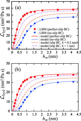
Figure 5: Two-dimensional hydrodynamic permeance ${\cal L}_{\rm hyd}$ versus the inter-layer distance $h_{m}$ obtained by means of the LBM, in comparison with the continuum model in Eq. (4) (Eq. (5) for the perfect slip boundary condition.) The geometrical parameters are $D_{m}=1$ nm, $L_{m}=3.7$ nm, $\ell=0.31$ nm, and $N=2$ in panel (a) or $N=3$ in panel (b).

IV Comparison of MD results with hydrodynamic predictions

We now gather the various results and compare the water permeance obtained using the MD simulations in Sec. II with the model prediction in the previous section.

IV.1 Flow parameters

The comparison between the MD simulations and hydrodynamic calculation requires to define several quantities: the viscosity, the slip length $b$, and the corrections $\delta D$ and $\delta h$, which determine the effective lengths $D_{m}$ and $h_{m}$, respectively. The value of the viscosity used in the hydrodynamic model is taken from Ref. González and Abascal, 2010. It is evaluated for the interaction potential used in the present study. In order to determine unambiguously the values of $b$, $\delta D$ and $\delta h$, we consider alternative geometries: (i) the flow through a slit across a single layer graphene, as well as (ii) a slab geometry with water confined between two graphene walls to determine the slip length.

First, in Fig. 6(a), the permeance of an independent nanoslit across a single layer of graphene is plotted versus the slit width. These data are compared to the corresponding continuum model ${\cal L}_{\rm hyd}^{(1)}$ given in Eq. (1), in order to estimate the effective hydrodynamic width $D_{m}$. The results of Eq. (1) for a few values of $\delta D$ are shown. If one sets $D_{m}=D$ (or $\delta D=0$), the permeance is overestimated, as expected considering the excluded volume around the carbon atoms. Clearly, the choice of $\delta D=0.5$ nm does approximate well the excluded volume and yields a precise prediction for the permeance. The gap correction $\delta h$, which also accounts for exclusion effects, is expected to be quantitatively similar to $\delta D$, i.e. $\delta h\approx 0.5$ nm. This was actually checked in the comparison between the MD results for the flux in the slab geometry described below and the hydrodynamic model ${\cal L}_{\rm hyd}^{(3)}$ in Eq. (3) with different values of $\delta h$ (not shown). As a result, the choice of $\delta h=0.5$ nm (or $h_{m}=h-0.5$ nm) is found to give a good agreement. We note that the values for the exclusion volume determined here in terms of the measurement of the flux, i.e. $\delta D=\delta h=0.5$ nm, are consistent with the density profile shown in Fig. 2(b), and a relevant discussion is also found in Ref. Gravelle et al., 2014. In the following, we set accordingly $\delta D=\delta h=0.5$ nm (or $D_{m}=D-0.5$ nm, $h_{m}=h-0.5$ nm) to compare with MD data in Fig. 3.

In order to estimate the slip length $b$, we next consider a water slab confined between two parallel graphene sheets with no slit. We examine the friction coefficient $\lambda$ between the water and the graphene walls by means of the methods described in Ref. Falk et al., 2012. The slip length is then evaluated from the friction coefficient via the relation $b=\eta/\lambda$. The friction coefficient is obtained using two different methods. First, we measure the fluctuation of the friction force $F$ (force acting in the lateral direction to the water form the graphene) at an equilibrium state without external force, in order to obtain the friction coefficient through the Green–Kubo formula. Bocquet and Barrat (1994, 2007) Second we measure the average slip velocity $v$ of water during a non-equilibrium MD simulation with a constant force acting on each water molecule in the direction parallel to the graphene sheet. The friction coefficient is then directly evaluated using the relation $\lambda=-F/Av$ ($A$ is the area of the sheet). Figure 6(b) shows the obtained friction coefficient as a function of the gap between the two sheets. As in Ref. Falk et al., 2012, the friction coefficient is measured to be independent of the gap. The resulting slip length is $b=30$ nm, which is also consistent with the previous results, Thomas and McGaughey (2008); Falk et al. (2012); Kannam et al. (2012) and this value is used in Fig. 3.

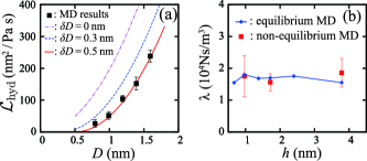
Figure 6: (a) Two-dimensional hydrodynamic permeance of an independent slit obtained using the MD simulation measured at $\Delta P=1000$ bar, in comparison with the continuum model in Eq. (1) with different values of $\delta D$. See the caption of Fig. 2 for the meaning of the error bar. (b) Friction coefficient $\lambda$ for the slab geometry of the gap $h$. The results of the equilibrium and non-equilibrium MD simulations are shown. The error bar indicates the standard deviation for the data obtained with different values of the applied body force.

Table 1: Model parameters.

slip length $b$	$30$ nm
slit width correction $\delta D$	$0.5$ nm
inter-layer distance correction $\delta h$	$0.5$ nm

Table 1 lists the model parameters for Eq. (4) determined from the discussion above, and Fig. 7 shows the comparison of the MD results for $N\geq 2$ with the model prediction using these parameters. The geometrical parameters are $L=6.82$ nm, $h=1$ nm, and $D=1.42$ nm. The MD results are the permeance evaluated at $\Delta P=1000$ bar. Even for the very complex geometry with many entrances and gaps up to $N=7$, the permeance is well predicted by the model. A typical profile of the flow velocity in the case of $N=3$ is also shown in Fig. 8, in comparison with the corresponding profile obtained using the LBM. As mentioned above, since the slip length is very large and the model is almost identical to the perfect-slip case, the decreasing of the permeance as $N$ is caused by the increase of the number of entrances, rather than the increase of the length of the flow path.

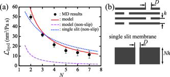
Figure 7: (a) Two-dimensional hydrodynamic permeance ${\cal L}_{\rm hyd}$ versus number of graphene layers $N$. The symbol indicates the MD results evaluated at $\Delta P=1000$ bar, and the lines indicate the model predictions. The dashed blue line is the predicted permeance of an single-slit membrane depicted in panel (b). The geometrical parameters are $L=6.82$ nm, $h=1$ nm, and $D=1.41$ nm. See the caption of Fig. 2 for the meaning of the error bar.

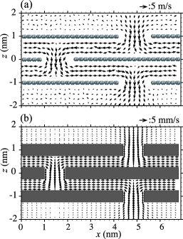
Figure 8: Flow velocity profiles in the $x$-$z$ plane. (a) MD result for the case of $L=6.82$ nm, $h=1$ nm, $D=1.41$ nm, and $N=3$ obtained applying the pressure difference $\Delta P=1000$ bar, and (b) the corresponding profile obtained using the LBM with the perfect-slip boundary condition applying $\Delta P=1$ bar. The scale of the vector is shown above each panel.

IV.2 Multi-layered graphene membrane: MD versus hydrodynamics

We can now discuss the MD results for the permeance, as shown in Fig. 3, in light of hydrodynamic predictions in Eq. (4).

A first result is that the model with the no-slip boundary condition ($b=0$) greatly underestimates the permeance for $h\leq 2$ nm. Now the hydrodynamic model with $b=30$ nm for the slip length, as obtained above, gives a good agreement with the MD results for various inter-layer distance and for the two typical conditions in Fig. 3. Altogether this comparison confirms that the continuum framework provides a quantitative prediction for the permeance down to sub-nanometer gaps between the layers, if the model parameters are appropriately chosen.

More into the details of the results, one observes two regimes for the permeance in Fig. 3. One is the range $h>D$ where the flow is dominantly limited by the resistance at the entrance of the nanoslits (${\cal L}_{\rm hyd}^{(1)}$). The dependence on $h$ is thus relatively weak in this regime. On the other hand, the resistance at the entrance of the gap (${\cal L}_{\rm hyd}^{(2)}$) starts to limit the flow at $h\sim D$ and the permeance rapidly decreases as decreasing $h$ in the range $h<D$. The quantitative explanation of this scenario is given by the plot of the decomposed permeances in the inset of Fig. 3(b), and consequently the hydrodynamic model in Eq. (4) accurately captures this two-regime behavior. The validity of this hydrodynamic model in atomic scale is further supported by the very recent MD results for a similar geometry in Ref. Muscatello  et al., 2016 (published after the submission of the present work,) where a detailed molecular analysis of the hydrogen-bonding shows a sufficient mixing of water even for a small inter-layer distance down to $0.6$ nm, thus promoting hydrodynamic behavior.

Finally, in Fig. 7, the MD results for the multi-layer graphene membrane are compared to the permeance of an artificial single-slit, solid, membrane with thickness $Nh$. We define the permeance of the single-slit geometry as ${\cal L}_{\rm hyd}=(1/{\cal L}_{\rm hyd}^{(1)}+1/{\cal L}_{\rm hyd}^{(3)})^{-1}$ with $L_{m}$ and $h_{m}$ in Eq. (3) replaced by $Nh$ and $D_{m}$, respectively, and the boundary condition inside the slit is assumed to be that of no-slip condition ($b=0$). The permeance of this single-slit no-slip membrane is found to be comparable to that of the multi-layered graphene membrane. This means that, in the nano-structured membrane, the slip effect becomes significant and compensates the reduction of the permeance due to the labyrinthine complexity of the geometry. The significance of this effect is clear if one compares with the model prediction for the multi-layer membrane with the no-slip condition, as shown in Fig. 7 (bottom curve). Also, if one assumes $b=30$ nm for the single-slit case, the permeance is far larger than that in Fig. 7(a) because the main resistance is that of the single slit entrance.

Table 2: Comparison with experimental data.

	${\cal L}_{\rm A}^{\rm(experiment)}$	${\cal L}_{\rm A}^{\rm(model)}$	$h\,^{\rm a)}$	$D\,^{\rm b)}$	$L\,^{\rm b)}$	$N\,^{\rm a)}$
	(nL$/$m2Pa s)	(nL$/$m2Pa s)	(nm)	(nm)	(nm)
Xia et al.Xia et al. (2015)	$75.3$	$74.2$	$1.38$	$10$	$190$	$14$
$\uparrow$	$30.6$	$23.3$	$0.99$	$10$	$190$	$14$
Hu & MiHu and Mi (2013)	$62.9$	$62.3$	$1.75$	$10$	$315$ c)	$15$
Nair et al.Nair et al. (2012)	$10^{4}$	$0.19$	$1.0$	$10$	$1000$ c)	$100$

^a) taken from the references. ^b) estimated. ^c) estimated within the range provided in the references.

V Concluding remarks

In the present study, we investigated the hydrodynamic permeance of the water flow past the geometrically complex graphene-based membrane, by means of a combined analysis of the atomic-scale MD simulation and the continuum hydrodynamics framework. To construct the continuum model, we first defined the coarse-grained geometry approximating the original configuration of the atomic-scale graphene walls. Then the derived simplified model was proven to be sufficiently accurate within the continuum description, by comparing with the results of the direct numerical simulation using the lattice Boltzmann method. The parameters appearing in the model from the coarse-graining of the geometry, i.e., the slip length $b$ and the corrections to the slit width $\delta D$ and to the gap $\delta h$, were identified as in Table 1, by means of the MD simulations of the decomposed basic problems. With these values of the parameters, the model was shown to predict the full MD results as shown in Figs. 3 and 7.

An important consequence in the present study is that the continuum description is still valid for explaining the small-scale flows down to sub-nanometers, if the parameters are carefully chosen. This is a benchmark result which is essential to examine critically the experimental results reported for graphene-based membranes. An example is shown in Table 2, where the experimental results reported in Refs. Xia et al., 2015; Hu and Mi, 2013; Nair et al., 2012 are compared to the present model in Eq. (4). In the table, the water permeance per unit area of the membranes ${\cal L}_{\rm A}$ is listed, which is related to ${\cal L}_{\rm hyd}$ via ${\cal L}_{\rm A}={\cal L}_{\rm hyd}/L$. The present model exhibits good agreements with the experimental results in Refs. Xia et al., 2015; Hu and Mi, 2013, if the values of the geometrical parameters $D$ and $L$ are estimated within reasonable ranges, for which the precise values are unavailable in the references. (Since the geometries in the experiments are not strictly identical to the setup considered in the present study, the tuned values are regarded as the effective values for the experimental membranes that include random configurations. Note that in the regime of $D\gg h$, the permeance is barely sensitive to $D$.)

On the other hand, the present model strongly underestimates the result of Ref. Nair et al., 2012, suggesting that other effects may contribute to the giant permeance measured in Ref. Nair et al., 2012. A possible reason lies in the driving force used to measure the permeability. While in Refs. Xia et al., 2015; Hu and Mi, 2013 it is obtained with an imposed pressure drop, in Ref. Nair et al., 2012 water evaporation is used to measure the permeability. In this case, a very large capillary contribution to the disjoining pressure due to the nanometric inter-layer distance Gravelle et al. (2016) may add up to the imposed pressure drop and increase accordingly the driving force. This supplementary capillary pressure would lead to a strong flow in spite of a small imposed pressure drop, thus affecting the extracted value of the permeance. Note that reversely the independent knowledge of the permeance in this system would allow to get much insights into the capillary pressure and disjoining effects at small scales. Gravelle et al. (2016) This suggests further experimental work along these lines.

One of extensions of the present study would be investigating flow properties of fluids other than water, and exploring the performance as filtration and separation membranes. A validation of the model prediction, by comparing with the permeance observed experimentally under a well-defined situation, would also be an important topic.