Noise-Resistant Quantum Teleportation, Ansibles, and the No-Projector Theorem

Abstract

A method is presented for achieving entanglement-free teleportation of a quantum state subject to any quantum noise. We apply this as a light-speed noise-resistant communicator, but also treat the possibility of a quantum ansible, a device for effectively superluminal communication and quantum broadcasting. The results suggest a “no-projector theorem” analogous to the no-cloning theorem. We then show how to build a pseudo-ansible for connection-free light-speed communication.

I Introduction

Since the birth of special relativity in 1905 Einstein (1905); Einstein et al. (1952), many have tried to break the classical light-speed limit to achieve superluminal communication. The most popular attempts use entanglement and quantum cloning Herbert (1979, 1982), but such methods have been proven impossible Bussey (1982); Westmoreland and Schumacher (1998); Bruss et al. (2000); Simon et al. (2001).

Here, we propose a new communication method that pairs two big ideas: entanglement-free quantum teleportation to send information as a state, and quantum error correction (QEC) to protect the state during teleportation. We call this noise-resistant quantum teleportation (NRQT). In one realization, it is light-speed limited and requires a physical connection. However, the theory also suggests that if true projectors are possible, then information could be sent faster than light, without violating special relativity. We can call any device that achieves this an ansible, a term coined by science-fiction author Ursula K. Le Guin for the idea proposed by earlier authors like Isaac Asimov, inspired by Einstein. This suggests a “no-projector theorem,” but also indicates that a connection-free light-speed pseudo-ansible is possible.

Figure 1: (color online) Unassisted QEC (UQEC) combined with teleportation to achieve NRQT. $\mathcal{E}$ is any error channel, $L_{j}$ and $L_{j}^{{\dagger}}$ are synchronized encoding/decoding operations, and $\mathcal{R}$ is a recovery channel, all in the space of $\rho$. Alice can send any message to Bob, regardless of noise.

The protection against quantum noise comes from a new form of QEC that is capable of correcting all errors, without help from ancillas, called unassisted quantum error correction (UQEC), depicted in Fig.1. UQEC both protects against noise and enables the teleportation, but is impractical for quantum computation (see App.A).

To present ideas organically, Sec.II reviews UQEC and its role in NRQT, showing how the existence of projectors leads to effective superluminality. Then, Sec.III shows how to build an ansible if true projectors could be realized, motivating a “no-projector theorem” in Sec.IV. Finally, Sec.V shows how to build a pseudo-ansible for connection-free light-speed communication.

II UQEC Applied to Noise-Resistant Quantum Teleportation

Unassisted quantum error correction (UQEC) in its full form can protect any quantum state from any noise channel, as shown in App.A. However, for conceptual simplicity we begin by reviewing a special case called limited-direct UQEC, which only protects a limited family of states from all noise. We then discuss how to realize the process and examine the crucial role of projectors.

II.1 Overview of Unassisted Quantum Error Correction

The process of limited-direct UQEC starts by only considering as input families of states with the form

$$\rho\equiv\rho_{(\bm{\theta})}\equiv\sum\limits_{j=1}^{n}{\lambda_{j}(\bm{\theta})|e_{j}\rangle\langle e_{j}|},$$ (1)

where $\{|e_{j}\rangle\}$ is a set of $n$ orthonormal states that are the defining constant of the family $\rho_{(\bm{\theta})}$, and where $\lambda_{j}\equiv\lambda_{j}(\bm{\theta})\in[0,1]$ are eigenvalues where $\sum\nolimits_{j=1}^{n}{\lambda_{j}}=1$, so the family’s free parameters are $\bm{\theta}\equiv\{\theta_{1},\ldots,\theta_{n-1}\}\in[0,{\textstyle{\pi\over 2}}]$.

Given input $\rho_{(\bm{\theta})}$, we can get limited-direct UQEC as

$$\rho_{(\bm{\theta})}=\sum\limits_{j=1}^{n}{\sum\limits_{q=1}^{n}{\sum\limits_{k}{L_{j}^{{\dagger}}R_{q}E_{k}L_{j}\rho_{(\bm{\theta})}L_{j}^{{\dagger}}E_{k}^{{\dagger}}R_{q}^{{\dagger}}L_{j}}}},$$ (2)

where we define encoding and recovery operators as

$$L_{j}\equiv|\psi\rangle\langle e_{j}|\;\;\text{and}\;\;R_{q}\equiv|\psi\rangle\langle\phi_{q}|,$$ (3)

where $|\psi\rangle$ is the reference state, which is any pure state, $\{|\phi_{q}\rangle\}$ is any orthonormal complete basis, $\{|e_{j}\rangle\}$ is the constant set of orthonormal eigenstates defining $\rho_{(\bm{\theta})}$, and $\{E_{k}\}$ are Kraus operators of noise channel $\mathcal{E}$ where $\sum\nolimits_{k}\!E_{k}^{{\dagger}}E_{k}=I$. Operators like those in (3) can be decomposed as a unitary operation and rank-$1$ projector, as shown in Sec.II.4.3. See App.A for a derivation of (2).

Next, to see how (2) enables us to protect any family of states $\rho_{(\bm{\theta})}$ in the form of (1) from any quantum noise channel, we will look at a single-qubit example.

II.2 Single-Qubit Example of UQEC

Here, we do a step-by-step example showing that all possible input states of a certain family can be recovered from all possible error channels acting on one qubit ($n=2$). For simplicity, let $\{|u\rangle\}$ be computational basis kets generically labeled starting on $1$ as $\{|1\rangle,\ldots,|n\rangle\}$.

First, define the state family of constant eigenstates by picking $\{|e_{j}\rangle\}\equiv\{|1\rangle,|2\rangle\}$, so that

$$\rho\equiv\rho_{(\theta)}\equiv\sum\limits_{j=1}^{2}{\lambda_{j}|e_{j}\rangle\langle e_{j}|}=c_{\theta}^{2}|1\rangle\langle 1|+s_{\theta}^{2}|2\rangle\langle 2|,$$ (4)

where $c_{\theta}\equiv\cos(\theta)$ and $s_{\theta}\equiv\sin(\theta)$. Then, choosing $|\psi\rangle\!=\!|1\rangle$ and $\{|\phi_{q}\rangle\}\equiv\{|1\rangle,|2\rangle\}$, where $|1\rangle\!\equiv\!\binom{1}{0}$ and $|2\rangle\!\equiv\!\binom{0}{1}$, (3) gives both the encoding and recovery operators as

$$L_{1}=R_{1}=\left(\!{\begin{array}[]{*{20}c}1&0\\ 0&0\\ \end{array}}\!\right)\;\;\text{and}\;\;\,L_{2}=R_{2}=\left(\!{\begin{array}[]{*{20}c}0&1\\ 0&0\\ \end{array}}\!\right)\!,$$ (5)

where Sec.II.4.3 explains their physical implementation.

The first step in the protection procedure is to randomly choose and apply one of the $L_{j}$ to $\rho$, keeping in mind that later, we will also have to apply its adjoint $L_{j}^{{\dagger}}$. A physical process for this is given in Sec.II.4.2, but for now, the possible results of the encoding step are

$$L_{j}\rho L_{j}^{{\dagger}}={\lambda_{j}}\!\left(\!{\begin{array}[]{*{20}c}1&0\\ 0&0\\ \end{array}}\!\right)\!,$$ (6)

where the coefficients $\lambda_{j}\equiv\langle e_{j}|\rho|e_{j}\rangle$ are given by

$$\lambda_{1}=\rho_{1,1}=c_{\theta}^{2}\;\;\;\text{and}\;\;\;\lambda_{2}=\rho_{2,2}=s_{\theta}^{2},$$ (7)

where $\rho_{a,b}\equiv\langle a|\rho|b\rangle$. Then one of the $E_{k}$ acts, producing

$$E_{k}L_{j}\rho L_{j}^{{\dagger}}E_{k}^{{\dagger}}=\lambda_{j}\left(\!{\begin{array}[]{*{20}c}{|(E_{k})_{1,1}|^{2}}&{(E_{k})_{1,1}(E_{k})_{2,1}^{*}}\\ {(E_{k})_{2,1}(E_{k})_{1,1}^{*}}&{|(E_{k})_{2,1}|^{2}}\\ \end{array}}\!\right)\!,$$ (8)

where again, $(E_{k})_{a,b}\equiv\langle a|E_{k}|b\rangle$. Next we randomly apply one of the recovery operators, producing

$$R_{q}E_{k}L_{j}\rho L_{j}^{{\dagger}}E_{k}^{{\dagger}}R_{q}^{{\dagger}}=\lambda_{j}|(E_{k})_{q,1}|^{2}\left({\begin{array}[]{*{20}c}1&0\\ 0&0\\ \end{array}}\right)\!.$$ (9)

Then, applying the matched decoder $L_{j}^{{\dagger}}=|e_{j}\rangle\langle 1|$ yields

$$L_{j}^{{\dagger}}R_{q}E_{k}L_{j}\rho L_{j}^{{\dagger}}E_{k}^{{\dagger}}R_{q}^{{\dagger}}L_{j}=\lambda_{j}|(E_{k})_{q,1}|^{2}|e_{j}\rangle\langle e_{j}|.$$ (10)

Now, since we don’t know which $E_{k}$ happened, or which $R_{q}$ was applied, or which pair $\{L_{j},L_{j}^{{\dagger}}\}$ was used, then before we look at the result, the potentially unnormalized state is the sum over all possible results, as

$$\sum\limits_{j=1}^{2}\sum\limits_{q=1}^{2}{\sum\limits_{k}{L_{j}^{{\dagger}}R_{q}E_{k}L_{j}\rho L_{j}^{{\dagger}}E_{k}^{{\dagger}}R_{q}^{{\dagger}}L_{j}}}=C\sum\limits_{j=1}^{2}\lambda_{j}|e_{j}\rangle\langle e_{j}|,$$ (11)

where $C$ is an “error-dependent” scalar, defined as

$$C\equiv\sum\limits_{q=1}^{n}{\sum\limits_{k}{|(E_{k})_{q,1}|^{2}}}.$$ (12)

Appendix A.1 proves that $C=1$ for all channels, but here we keep it. Now we see that the matrix to the right of $C$ in (11) only contains information about $\rho$, and putting (4) into (11) and normalizing (unnecessarily) gives

$${\textstyle{{1}\over{\text{tr}(C\rho)}}}\sum\limits_{j=1}^{2}{\sum\limits_{q=1}^{2}{\sum\limits_{k}\!{L_{j}^{{\dagger}}R_{q}E_{k}L_{j}\rho L_{j}^{{\dagger}}E_{k}^{{\dagger}}R_{q}^{{\dagger}}L_{j}}}}=\rho,$$ (13)

which is identical to the input state, as desired. Notice that no ancilla systems are needed, and this same method works for all $n$-level systems, even with nonlocal noise.

II.3 Numerical Demonstration of UQEC

Here, we look at a numerical test to see that UQEC works, but see App.A for a proof that it always works. Figure 2 subjects an arbitrary qutrit $\rho$ to an arbitrary noise channel $\mathcal{E}(\sigma)\equiv\sum\nolimits_{k}E_{k}\sigma E_{k}^{{\dagger}}$.This qutrit is treated

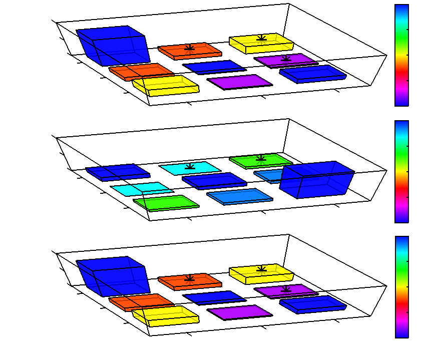
Figure 2: (color online) Limited-direct UQEC on an arbitrary qutrit in an arbitrary noise channel. These plots depict density-matrix representations of the states. For each matrix element, labeled by row indices on the bottom left and column indices on the bottom right, the height of the box gives the magnitude, the color represents the phase-angle magnitude, and an asterisk on top indicates a negative phase angle. (a) shows input $\rho$, (b) shows damaged state $\rho_{E}$ resulting from no protection, and (c) shows recovered state $\rho_{R}$ resulting from full protection. Note that $\rho_{R}=\rho$ exactly.

as part of a constant family $\rho_{(\theta_{1},\theta_{2})}$ by using its eigenstates to construct $L_{j}$. Figure 2 then compares $\rho$ to the error-damaged state $\rho_{E}\equiv\mathcal{E}(\rho)$, and to the recovered state $\rho_{R}\equiv\sum\nolimits_{j=1}^{n}\sum\nolimits_{q=1}^{n}{\sum\nolimits_{k}{L_{j}^{{\dagger}}R_{q}E_{k}L_{j}\rho L_{j}^{{\dagger}}E_{k}^{{\dagger}}R_{q}^{{\dagger}}L_{j}}}$, which includes the effects of $\mathcal{E}$.

II.4 How to Realize the Quantum Operations for Noise-Resistance

Here we discuss the fine points of the UQEC procedure, focusing on practical methods of implementation, to see how it applies to noise-resistant quantum teleportation (NRQT), and to identify the problem with projectors.

II.4.1 Classical Generation of Quantum Operations

To prepare for later discussions, here we briefly review quantum operations Hellwig and Kraus (1969, 1970); Choi (1975); Kraus (1983). A dimension-preserving quantum operation $\mathcal{F}(\rho)$ maps states in the space of $\rho$ to other states $\rho^{\prime}\equiv\mathcal{F}(\rho)$ in the same space, as

$$\mathcal{F}(\rho)=\sum\limits_{k=1}^{n_{F}}{F_{k}\rho F_{k}^{{\dagger}}},$$ (14)

where $\{F_{k}\}$ is a set of $n_{F}$ Kraus operators in the space of $\rho$, obeying Kraus completeness,

$$\sum\limits_{k=1}^{n_{F}}{F_{k}^{{\dagger}}F_{k}}=I,$$ (15)

where the identity $I$ is also in the space of $\rho$.

There are many ways to physically interpret quantum operations, but the one of interest for NQRT is as follows.

State-Free Interpretation:  Apply all $F_{k}$ with equal probabilities $p_{k}^{\prime}\equiv{\textstyle{1\over{n_{F}}}}$, and then normalize the result as

$$\mathcal{F}(\rho)=\frac{\sum\nolimits_{k=1}^{n_{F}}{{\textstyle{1\over{n_{F}}}}F_{k}\rho F_{k}^{{\dagger}}}}{\text{tr}(\sum\nolimits_{k=1}^{n_{F}}{{\textstyle{1\over{n_{F}}}}F_{k}\rho F_{k}^{{\dagger}}})}=n_{F}\sum\limits_{k=1}^{n_{F}}{{\textstyle{1\over{n_{F}}}}F_{k}\rho F_{k}^{{\dagger}}}.$$ (16)

The normalization is state-independent because of (15) and the fact that $\text{tr}(\rho)=1$, which together enable $\text{tr}(\sum\nolimits_{k=1}^{n_{F}}{{\textstyle{1\over{n_{F}}}}F_{k}\rho F_{k}^{{\dagger}}})={\textstyle{1\over{n_{F}}}}\sum\nolimits_{k=1}^{n_{F}}{\text{tr}(\rho F_{k}^{{\dagger}}F_{k})}={\textstyle{1\over{n_{F}}}}$.

Thus, we will use the State-Free Interpretation to treat all quantum operations as applications of Kraus operators with equal probability, followed by normalization.

Another ingredient useful for classical implementation of UQEC is a method for probabilistic application of operations. This is simpler than it sounds; just use a random or true random number generator (TRNG).

The scenario goes like this: As shown in Fig.3, a device containing a TRNG internally produces a number $k$ between $1$ and $n_{F}$, where the TRNG produces any of these numbers with equal probability. The device applies the operation $F_{k}$ to the system in the input state $\rho$, but no information about which operation was applied is allowed to leave the device. Then, after the operation was applied, since we know any one of the $F_{k}$ could have been applied, but we do not know which, then the state of the output system is $\mathcal{F}(\rho)=\sum\nolimits_{k=1}^{n_{F}}{F_{k}\rho F_{k}^{{\dagger}}}$, thus classically realizing some intended quantum operation $\mathcal{F}(\rho)$.

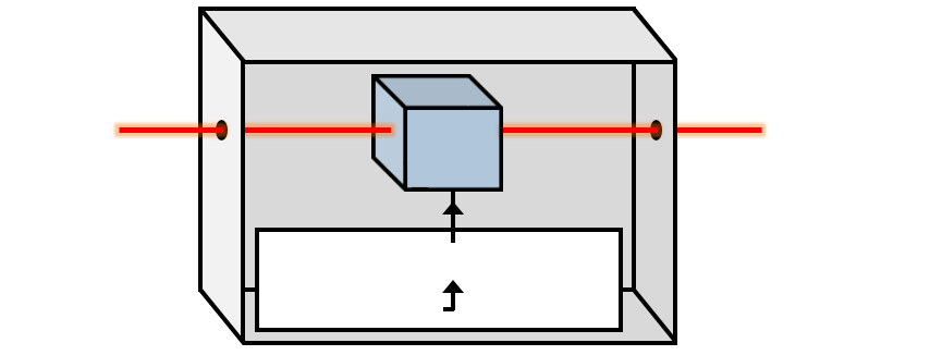
Figure 3: (color online) Schematic of classical implementation of the State-Free Interpretation of a quantum operation $\mathcal{F}(\rho)=\sum\nolimits_{k=1}^{n_{F}}{F_{k}\rho F_{k}^{{\dagger}}}$. A closed box contains a true random number generator (TRNG) that makes random number $k$, selects the $k$th operation $F_{k}$, and applies it to input state $\rho$. Since each $F_{k}$ has equal probability of being applied, and since observers outside the box do not know which $F_{k}$ was applied, the output state is $\mathcal{F}(\rho)$, the normalized sum of all possible results $\{F_{k}\rho F_{k}^{{\dagger}}\}$.

Note that this involves only classical probability, and thus it is our ignorance of which operation was applied that “creates” the classical mixture of all the operations acting on the input state. However, this step-function method only works perfectly if the Kraus operators can be applied alone deterministically, as Sec.IV explains.

Alternatively, we could make quantum operations by reducing from larger systems, but this classical method is what lets us synchronize the encoders and decoders.

II.4.2 Implementation of Index-Linked Operations

The peculiar thing about (2) is its index-linked operators, the $j$-indexed pairs in $L_{j}^{{\dagger}}R_{q}E_{k}L_{j}$. While App.A.2 proves the existence of physical index-linked operations, here we simply show one way to realize them, in Fig.4.

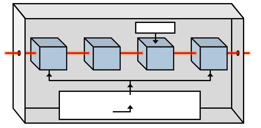
Figure 4: (color online) Schematic of an implementation of limited-direct UQEC. A closed box contains a true random number generator (TRNG) that makes random number $j$, selects the $j$th encoding/decoding pair $\{L_{j},L_{j}^{{\dagger}}\}$, and first applies $L_{j}$ to input state $\rho$. Then, error channel $\mathcal{E}$ randomly applies one of its errors $E_{k}$. Then, another TRNG selects and applies the $q$th recovery operator $R_{q}$. Finally, the other member $L_{j}^{{\dagger}}$ of the $\{L_{j},L_{j}^{{\dagger}}\}$ pair is applied, and since information about which operators were applied inside the box is not learned by observers outside, the output state is $\rho$, from (2).

II.4.3 How to “Realize” the Individual Kraus Operators

Recall from (3) that we need operators of the form $|\psi\rangle\langle\phi|$, which are in general both nonHermitian and nonunitary. To “realize” these, if we use the descending eigenvalue convention, such that eigenvalues of all states are labeled as $\lambda_{1}\geq\cdots\geq\lambda_{n}\geq 0$ where $\sum\nolimits_{k=1}^{n}{\lambda_{k}}=1$, then we can express $L_{j}\equiv|\psi\rangle\langle e_{j}|$ and $R_{q}\equiv|\psi\rangle\langle\phi_{q}|$ as

$$L_{j}=P_{|\psi\rangle}\epsilon_{|\psi\rangle}\epsilon_{|e_{j}\rangle}^{{\dagger}}\;\;\;\text{and}\;\;\;R_{q}=P_{|\psi\rangle}\epsilon_{|\psi\rangle}\epsilon_{|\phi_{q}\rangle}^{{\dagger}},$$ (17)

where $P_{|\psi\rangle}\equiv|\psi\rangle\langle\psi|$ is a projector, and $\epsilon_{|A\rangle}$ is the unitary descending-order eigenvector matrix of $|A\rangle\langle A|$, for which columns of $\epsilon_{|A\rangle}$ are eigenstates of $|A\rangle\langle A|$, and $\epsilon_{|A\rangle}^{{\dagger}}A\epsilon_{|A\rangle}=\Lambda_{|A\rangle}\equiv\text{diag}\{\lambda_{1},\ldots,\lambda_{n}\}$ is the diagonal eigenvalue matrix of $n$-level matrix $|A\rangle\langle A|$. Thus, each $L_{j}$ and $R_{q}$ can be “realized” by a unitary gate and projective filter. Note that $|e_{j}\rangle$ are eigenstates of $\rho$ and that $\epsilon_{|e_{j}\rangle}$ is the descending-order eigenvector matrix of $|e_{j}\rangle\langle e_{j}|$.

If we choose $|\psi\rangle$ as the first computational basis state $|1\rangle$, then we can set $\epsilon_{|\psi\rangle}=\epsilon_{|1\rangle}=I$, and (17) simplifies to

$$L_{j}=P_{|1\rangle}\epsilon_{|e_{j}\rangle}^{{\dagger}}\;\;\;\text{and}\;\;\;R_{q}=P_{|1\rangle}\epsilon_{|\phi_{q}\rangle}^{{\dagger}}.$$ (18)

As Sec.II.4.4 explains, true projectors may be difficult (or impossible) to achieve, since absorptive projective filters such as polarizers do not produce scalar zero from orthogonal input, but instead produce the vacuum state. However, for light-speed limited (light-limited) communication, absorptive projectors will be adequate.

II.4.4 True Projectors Cannot be Implemented with Absorptive Projective Filters

Consider a state in an orthonormal basis $\{|\widetilde{1}\rangle,|\widetilde{2}\rangle\}$ as

$$|\psi\rangle=d|\widetilde{1}\rangle+e|\widetilde{2}\rangle,$$ (19)

where $|d|^{2}+|e|^{2}=1$, and the tilde is used since this basis is not necessarily composed of Fock states, but our results here will involve the Fock vacuum $|0\rangle$.

Now, a true projector, such as $P_{|\widetilde{1}\rangle}\equiv|\widetilde{1}\rangle\langle\widetilde{1}|$ causes

$$P_{|\widetilde{1}\rangle}|\psi\rangle\langle\psi|P_{|\widetilde{1}\rangle}=\left\{{\begin{array}[]{*{20}l}{|d|^{2}|\widetilde{1}\rangle\langle\widetilde{1}|;}&{|\psi\rangle\neq|\widetilde{2}\rangle}\\ {\;\;\;\;\;\;\;\;\,{\kern 0.4pt}0;}&{|\psi\rangle=|\widetilde{2}\rangle,}\\ \end{array}}\right.$$ (20)

before normalization, where the scalar zero in the second line is due to the fact that the overlap of the pass-state $|\widetilde{1}\rangle$ with an orthogonal state $|\widetilde{2}\rangle$ is zero; $\langle\widetilde{1}|\widetilde{2}\rangle=0$. (We write separate cases to make a point.)

However, as shown in App.B, absorptive projective filters (APFs) such as linear polarizers do not produce the scalar zero, and instead produce the vacuum state, as

$$P_{|\widetilde{1}\rangle}^{(\text{APF})}(|\psi\rangle\langle\psi|)=\!\left\{\!{\begin{array}[]{*{20}l}{|d|^{2}|\widetilde{1}\rangle\langle\widetilde{1}|+|e|^{2}|0\rangle\langle 0|;}&{|\psi\rangle\neq|\widetilde{2}\rangle}\\ {\;\;\;\;\;\;\;\;\;\;\;{\kern 2.6pt}|0\rangle\langle 0|;}&{|\psi\rangle=|\widetilde{2}\rangle,}\\ \end{array}}\right.$$ (21)

where the superscript APF reminds us that $P_{|\widetilde{1}\rangle}^{(\text{APF})}$ is really a selective absorption channel, which is why it merely produces the vacuum state in the orthogonal-input case.

Furthermore, the “pass-input” case of the APF is a mixture with the vacuum, whereas the corresponding case in (20) is a pure state.

As we will see in Sec.II.5, the ability of true projectors to produce scalar zero in the case of limited-direct UQEC is the key ingredient for the possibility of superluminal information transfer. Without it, one must use postselection, which we will discuss in Sec.II.6.

II.5 How to Achieve Noise-Resistant Quantum Teleportation with UQEC

Before using UQEC within a communication device, we need to incorporate quantum teleportation (QT), which we define as transfer of a quantum state from one spatial mode to another spatial mode, where mode simply means subsystem of the total Hilbert space. Since communication involves transfer of information from one place to another, then our noise-resistant quantum teleportation (NRQT) scheme must be able to maintain its UQEC action while achieving QT.

Traditionally, QT involves entanglement Bennett et al. (1993); Bouwmeester et al. (1997, 1998), but actually that is unnecessary. For example, an ideal (lossless) phase shifter acts as a kind of teleporter to flying states, at the cost of some phase factors, since it transmits the state from the spatial mode at its input port to the spatial mode at its output port (see App.C).

Here we will show that the UQEC process still works if we apply the recovery and decoding stages in a different location than the encoding. To start, suppose that our input is $\rho\otimes\upsilon$, and recalling that $L_{j}\equiv|\psi\rangle\langle e_{j}|$, the encoded state results are

$$\begin{array}[]{*{20}l}{L_{j}\rho L_{j}^{{\dagger}}\otimes\upsilon}&\!\!{=|\psi\rangle\langle e_{j}|\rho|e_{j}\rangle\langle\psi|\otimes\upsilon}\\ {}&\!\!{=\lambda_{j}|\psi\rangle\langle\psi|\otimes\upsilon},\\ \end{array}$$ (22)

where $\lambda_{j}\equiv\langle e_{j}|\rho|e_{j}\rangle$, and $|e_{j}\rangle$ are eigenstates of $\rho$. Now suppose that some noise channel $\mathcal{E}$ acts, possibly on both spatial modes, as

$$\mathcal{E}(L_{j}\rho L_{j}^{{\dagger}}\otimes\upsilon)=\lambda_{j}\mathcal{E}(\varsigma_{(\psi,\upsilon)}),$$ (23)

where $\varsigma_{(\psi,\upsilon)}\equiv|\psi\rangle\langle\psi|\otimes\upsilon$. Then, recalling that $R_{q}\equiv|\psi\rangle\langle\phi_{q}|$, if we apply the $R_{q}$ in the second spatial mode, and sum over all of them since we do not know which is applied at any time, we get

$$\mathcal{R}^{(2)}(\lambda_{j}\mathcal{E}(\varsigma_{(\psi,\upsilon)}))=\lambda_{j}\text{tr}_{2}(\mathcal{E}(\varsigma_{(\psi,\upsilon)}))\otimes|\psi\rangle\langle\psi|,$$ (24)

where $\mathcal{R}^{(2)}(\sigma)\equiv\sum\nolimits_{q=1}^{n}{(I^{(1)}\otimes R_{q})\sigma(I^{(1)}\otimes R_{q}^{{\dagger}}})$, and parenthetical superscripts are subsystem labels.

Finally, letting $\eta_{j}\equiv\mathcal{R}^{(2)}(\lambda_{j}\mathcal{E}(\varsigma_{(\psi,\upsilon)}))$ and recalling that $L_{j}\equiv|\psi\rangle\langle e_{j}|$, decoding in subsystem 2 gives results

$$(I^{(1)}\otimes L_{j}^{{\dagger}})\eta_{j}(I^{(1)}\otimes L_{j})=\text{tr}_{2}(E(\varsigma_{(\psi,\upsilon)}))\otimes\lambda_{j}|e_{j}\rangle\langle e_{j}|,$$ (25)

where we used the fact that $\lambda_{j}$ is a scalar to shift it to subsystem 2. Finally, summing over all the results gives

$$\sum\limits_{j=1}^{n}{(I^{(1)}\otimes L_{j}^{{\dagger}})\eta_{j}(I^{(1)}\otimes L_{j})}=\text{tr}_{2}(\mathcal{E}(\varsigma_{(\psi,\upsilon)}))\otimes\rho,$$ (26)

which we can also express as

$$\sum\limits_{j=1}^{n}{\sum\limits_{q=1}^{n}{\sum\limits_{k}\!{\Omega_{(j,q,k)}(\rho\otimes\upsilon)\Omega_{(j,q,k)}^{{\dagger}}}}}\!=\text{tr}_{2}(\mathcal{E}(\varsigma_{(\psi,\upsilon)}))\otimes\rho,$$ (27)

where $\Omega_{(j,q,k)}\equiv(I\otimes L_{j}^{{\dagger}}R_{q})E_{k}(L_{j}\otimes I)$, and $\text{tr}_{2}(\mathcal{E}(\varsigma_{(\psi,\upsilon)}))$ is some “garbage state” about which we do not care. Thus, we have shown that we can indeed successfully teleport $\rho$, the family of states of constant eigenstates $|e_{j}\rangle$, in the presence of any noise channel $\mathcal{E}$, even nonlocal noise over both modes of the teleportation.

We have just mathematically described superluminal communication…however, we will now see that how we realize the operators can cause major limitations.

II.6 NRQT via Passive Absorptive Projectors is Light-Speed Limited and Needs Lossless Connection

Notice that the crucial step in (25) was that the scalar $\lambda_{j}$ could slide from the sender’s mode to the receiver’s mode, thus enabling proper reconstruction of the input state in a different location.

Focusing on the encoding, the ideal action should be

$$\begin{array}[]{*{20}l}{L_{j}\rho L_{j}^{{\dagger}}}&\!\!{=|e_{1}\rangle\langle e_{j}|(\sum\limits_{k=1}^{n}{\lambda_{k}|e_{k}\rangle\langle e_{k}|})|e_{j}\rangle\langle e_{1}|}\\ {}&\!\!{=|e_{1}\rangle\langle e_{1}|\sum\limits_{k=1}^{n}{\lambda_{k}\delta_{j,k}}=\lambda_{j}|e_{1}\rangle\langle e_{1}|,}\\ \end{array}$$ (28)

where we have assumed the eigenbasis to be the computational basis, and the reference state is the first basis state. From this, we see that there should be an appearance of a scalar Kronecker delta to properly sift $\lambda_{j}$.

However, if we use absorptive projective filters, then as in App.B, letting $\rho_{L_{j}}^{(\text{APF})}\equiv P_{|e_{1}\rangle}^{(\text{APF})}(L_{j}\rho L_{j}^{{\dagger}})$ where $P_{|e_{1}\rangle}^{(\text{APF})}(\rho)\equiv\text{tr}_{2}((I\otimes A_{0}(\cdot))\rho_{\text{DR}})$ is a selective absorption channel where $\rho_{\text{DR}}\equiv U_{\text{PBS}}(\rho\otimes|0\rangle\langle 0|)U_{\text{PBS}}^{{\dagger}}$ is a dual-rail version of input $\rho$ such that the pass-state is kept in mode $1$, $U_{\text{PBS}}$ is a polarizing beam-splitter unitary, and $\mathcal{A}_{0}(\rho)=|0\rangle\langle 0|\;\forall\rho$ is the absorption channel (see Sec.III.1), we get

$$\begin{array}[]{*{20}l}{\rho_{L_{j}}^{(\text{APF})}}&\!\!{=P_{|e_{1}\rangle}^{(\text{APF})}\!\left({\epsilon_{|e_{j}\rangle}^{{\dagger}}(\sum\limits_{k=1}^{n}{\lambda_{k}|e_{k}\rangle\langle e_{k}|})\epsilon_{|e_{j}\rangle}}\right)}\\ {}&\!\!{=P_{|e_{1}\rangle}^{(\text{APF})}\!\left({\lambda_{j}|e_{1}\rangle\langle e_{1}|+\!\!\sum\limits_{k=1\neq j}^{n}\!\!\!{\lambda_{k}\epsilon_{|e_{j}\rangle}^{{\dagger}}|e_{k}\rangle\langle e_{k}|\epsilon_{|e_{j}\rangle}}}\right)}\\ {}&\!\!{=\lambda_{j}|e_{1}\rangle\langle e_{1}|+(1-\lambda_{j})|0\rangle\langle 0|,}\\ \end{array}$$ (29)

which shows that the only way to tell if the correct scalar is present is to wait for a nonvacuum event.

Thus, the use of absorptive projective filters (APFs) causes the communication of the scalar information $\lambda_{j}$ to be event-based and comparative to vacuum. Because the nonvacuum state must belong to a particle, this means that the use of APFs restricts us to light-speed communication, because we must wait for the particle to reach the receiver and thus communicate the nonvacuum event.

If we use passive APFs, such as polarizers, the need to wait for a nonvacuum event has another consequence; we must not allow the encoded state to experience further absorption, or else the whole state will be vacuum with unit probability as

$$\mathcal{A}_{0}(\rho_{L_{j}}^{(\text{APF})})=\lambda_{j}|0\rangle\langle 0|+(1-\lambda_{j})|0\rangle\langle 0|=|0\rangle\langle 0|,$$ (30)

which conveys no scalar information.

As Fig.5 shows, light-limited NRQT is possible. The restrictions of light-limiting and lossless transmission are honored by maintaining a line-of-sight connection and by restricting the error channel to the basis of the qubit. In this kind of setup, “all errors” means “all errors within the space of the input state.”

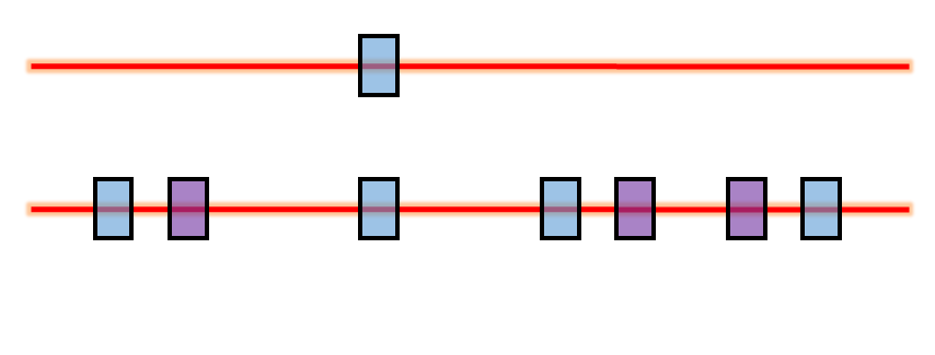
Figure 5: (color online) Example of light-limited noise-resistant quantum teleportation of $\rho=c_{\theta}^{2}|\widetilde{1}\rangle\langle\widetilde{1}|+s_{\theta}^{2}|\widetilde{2}\rangle\langle\widetilde{2}|$ as in (4), where $\{|\widetilde{1}\rangle,|\widetilde{2}\rangle\}$ are orthonormal single-photon polarization states. (a) Input $\rho$ is subjected to an emulated bit-flip channel in which 50% of the trials a half-wave plate (HWP) $U_{H}$ is placed, and 50% of the trials get nothing, yielding an output (if information about the HWP is ignored) of $\frac{1}{2}I$, the maximally mixed state. (b) The same emulated noise but now within the UQEC process using absorptive polarizers $P_{1}^{A}\equiv P_{|1\rangle}^{(\text{APF})}(\cdot)$, producing $\rho^{\prime}\equiv{\textstyle{1\over 4}}\rho+{\textstyle{3\over 4}}|0\rangle\langle 0|$. Postselecting for nonvacuum results, tomography on $\rho^{\prime}$ yields the message state $\rho$ in spite of having the same noise as (a).

Thus, using passive APFs rather than true projectors limits the teleportation to light speed, and imposes the further requirement that the sender and receiver be connected by a lossless transmission line.

Later we will see the particularly interesting alternative that if we use an active APF in the form of a detector at the sender, we can achieve “connection-free” postselected light-speed communication, where there still needs to be a path to send the classical postselection results, but the quantum part can and does get completely destroyed and therefore does not require a connection.

II.7 A Way to Achieve True Projectors

Mathematically, a joint-system two-qubit unitary that yields orthogonal projectors is the CNOT gate,

$$U_{\text{CNOT}}=\left({\begin{array}[]{*{20}c}1&0&0&0\\ 0&1&0&0\\ 0&0&0&1\\ 0&0&1&0\\ \end{array}}\right)\!.$$ (31)

Preparing the qubits as $\rho\otimes|\widetilde{1}\rangle\langle\widetilde{1}|$ so the target qubit is in the first computational basis state, then applying $U_{\text{CNOT}}$ and tracing over the target yields Kraus operators,

$$P_{|\widetilde{r}\rangle}=(I\otimes\langle\widetilde{r}|)U_{\text{CNOT}}(I\otimes|\widetilde{1}\rangle)=\{P_{|\widetilde{1}\rangle},P_{|\widetilde{2}\rangle}\},$$ (32)

where $P_{|\widetilde{r}\rangle}\equiv|\widetilde{r}\rangle\langle\widetilde{r}|$. Physically, although we only want one projector, we need both projectors in (32) for Kraus completeness. However, we do not want both simultaneously, because then both sides of the communicator could not be synchronized. Therefore, suppose these projectors happen in different time bins of a time-bin qubit.

Figure 6 shows how to make a projector channel where the same true polarization projector appears to act at different times, so the only difference is the time-bin 2 scalar, easily dealt with by treating the input of time-bin 2 as if it were a bit-flipped version of that of time-bin 1.

Figure 6: (color online) Example of a time-separated true-projector channel (see App.D for details). A photon’s internal polarization and momentum qubits enter a deterministic CNOT Fiorentino and Wong (2004), then time-bin conversion Bussières et al. (2006) and reduction yield $\rho_{\text{CNOT}}=\rho_{1,1}|\widetilde{1}_{\tau_{1}},0_{\tau_{2}}\rangle\langle\widetilde{1}_{\tau_{1}},0_{\tau_{2}}|\!+\!\rho_{2,2}|0_{\tau_{1}},\widetilde{1}_{\tau_{2}}\rangle\langle 0_{\tau_{1}},\widetilde{1}_{\tau_{2}}|$.

In Sec.V, we will see that while (32) does achieve true projectors, it still leads to ansible failure.

II.8 Insulating UQEC Enables Locally Generated Superposition Scalars

Another possible problem for an ansible is the meaning of the scalars based on how the input state was made.

If we create $\rho$ as a step-function of pure states, then scalars $\lambda_{j}$ are just statistical representations of classical events. However, if we instead obtain $\rho$ as the reduced state from the pure state of a larger system, then scalars $\lambda_{j}$ are directly inherited from pure-state superposition scalars, and are products of wave-function overlaps.

However, since the momentum ancilla is for the projectors, and since deterministic preparation of two-qubit photonic states is difficult, it would be nice if we could just use local pure states as input, instead of reductions. That way we could harvest the superposition scalars directly. The problem is that limited-direct UQEC can only convey information with mixed-state input.

Fortunately, the method of insulating UQEC from App.E can handle all input states, not just those of known eigenstates. Therefore, by restricting ourselves to pure input states and insulating UQEC, we can guarantee locally-prepared superposition scalars in our input.

Appendix E gives the details of insulating UQEC, but the only procedural differences for one qubit are that we now need six encoding/decoding pairs, and the output state $\rho_{D}$ is isomorphic to the input $\rho$, meaning that an extra numerical computation called extraction must be done to obtain $\rho$ from $\rho_{D}$.

The important thing is that with insulating UQEC, $\rho$ can be pure, such as $\rho=|\xi\rangle\langle\xi|$, where

$$|\xi\rangle=c_{\theta}|\widetilde{1}\rangle+s_{\theta}e^{i\phi}|\widetilde{2}\rangle,$$ (33)

where $c_{\theta}\equiv\cos(\theta)$ and $s_{\theta}\equiv\sin(\theta)$. Then, using the overcomplete basis given in App.E, the information-carrying scalars are (instead of $\lambda_{j}$),

$$\begin{array}[]{*{20}l}{d_{1}={\textstyle{1\over 2}}(1+s_{2\theta}c_{\phi}),}&{d_{3}={\textstyle{1\over 2}}(1+s_{2\theta}s_{\phi}),}&{d_{5}=c_{\theta}^{2},}\\ {d_{2}={\textstyle{1\over 2}}(1-s_{2\theta}c_{\phi}),}&{d_{4}={\textstyle{1\over 2}}(1-s_{2\theta}s_{\phi}),}&{d_{6}=s_{\theta}^{2},}\\ \end{array}$$ (34)

which all obey $d_{j}\geq 0$, so the quantum operation is physical, and most importantly, these scalars are directly inherited from the pure superposition scalars of (33), provided that we use true projectors.

Thus we now have a strategy for locally producing pure input states that ensure our UQEC operation only uses superposition scalars, which may avoid the light-speed limits of event-based statistical scalars.

For simplicity, in everything that follows, we will use the limited-direct UQEC variables, since technically we can get superposition scalars in mixed states by reducing from a larger pure multiqubit system, but keep in mind the advantages of using insulating UQEC instead.

II.9 Vacuum/Single-Photon Basis Conversion

For single-photon (SP) qubits, the all-mode vacuum is not part of their Hilbert space, yet general noise channels can easily take the state outside the SP subspace.

One way to handle this is to force vacuum involvement by converting encoded results to vacuum. If we use the methods of Sec.II.8 and Sec.II.7, our encoded results are all proportional to the same reference state, such as

$$L_{j}\rho L_{j}^{{\dagger}}=\lambda_{j}|1\rangle\langle 1|\;\;\,\text{or}\;\;D_{j}\rho D_{j}^{{\dagger}}=d_{j}|1\rangle\langle 1|,$$ (35)

where the scalars are true overlaps of pure states and are not event-based. Then, it is easy to see that conversion to vacuum via total absorption $\mathcal{A}_{0}$ preserves the scalars,

$$\mathcal{A}_{0}(D_{j}\rho D_{j}^{{\dagger}})=d_{j}\mathcal{A}_{0}(|1\rangle\langle 1|)=d_{j}|0\rangle\langle 0|.$$ (36)

Later, we will see an example showing what happens at the receiver; the important point here is that (36) shows that (if projectors exist) no classical signal needs to leave the encoding half of the device, vacuum will suffice!

III How to Build an Ansible if True Lone Projectors were Possible

Supposing that true lone projectors could be realized, here we organically show how to build an ansible, a device for effectively superluminal communication.

III.1 Using NRQT for Communication in the Context of the Quantum Vacuum

For the purposes of communication by quantum states, suppose that we have some source of flying qubits capable of making a steady stream of identically prepared states. Also suppose that these states can be accurately measured by tomography in reasonable amounts of time. We will further suppose that our qubits are optical, and therefore the first thing we must confront is how we can achieve NRQT in the context of the quantum vacuum.

To begin, we define the attenuation channel as a variable-transmittivity beam splitter $B_{\theta}\equiv e^{\theta(a_{1}^{{\dagger}}a_{2}-a_{1}a_{2}^{{\dagger}})}$ of transmittivity $T$, where $a_{1}$ and $a_{2}$ are annihilation operators for modes $1$ and $2$, and $\cos(\theta)\equiv\sqrt{\,\!T^{\,{}^{\,}}\!\!}$, with vacuum in its auxiliary input (mode $2$), and reduced as

$$\mathcal{A}_{T}(\rho)\equiv\mathcal{A}_{\theta(T)}(\rho)\equiv\text{tr}_{2}(B_{\theta}(\rho\otimes|0^{(2)}\rangle\langle 0^{(2)}|)B_{\theta}^{{\dagger}}).$$ (37)

This model of loss acknowledges that total absorption never yields just “$0$”, but instead outputs the vacuum state $|0\rangle$, since absorption is just part of a unitary process on a larger Hilbert space.

Now suppose we must send a state $\rho$ over a lossy transmission line modeled as an ideal unitary phase shifter $U$ of any length, preceded by an attenuation channel $\mathcal{A}_{T}$ of any value $T$, as in Fig.7. Then the output is

$$\rho^{\prime}=U\mathcal{A}_{T}(\rho)U^{{\dagger}}.$$ (38)

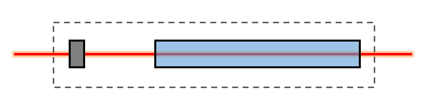
Figure 7: (color online) Lossy transmission line modeled as a variable neutral density filter (VNDF) represented by channel $\mathcal{A}_{T}(\rho)$ of (37) and an ideal phase shifter (PS) or fiber represented by unitary $U$. When $T\!=\!0$, $\mathcal{A}_{0}(\rho)\!=\!|0\rangle\langle 0|$, and $\rho^{\prime}\!\equiv\!U\mathcal{A}_{0}(\rho)U^{{\dagger}}\!=\!|0\rangle\langle 0|$, where $U\equiv e^{i\phi a^{{\dagger}}a}$, with annihilation operator $a$, and $\phi\equiv\omega\Delta t$ where $\omega$ is the field’s angular frequency and $\Delta t\equiv(n_{P}-n_{M})\frac{Z}{c}$ is the extra time delay for the field to propagate through the phase shifter of length $Z$ and refractive index $n_{P}$ beyond the time it would take in the surrounding medium of index $n_{M}$, where $c$ is the speed of light in vacuum. Any error channels inserted at any point in this sequence can all be combined with these elements as a single error channel to model a noisy transmission line, as well.

Note that although we use the standard single-mode model of a phase shifter, they are really two-mode devices, as mentioned earlier, which is partly responsible for the teleportation effect. See App.C for a two-mode model of a phase shifter.

The worst-case scenario is if the transmission probability is $T=0$, corresponding to placing a perfect absorber before the line, for which the output is

$$\rho^{\prime}=U\mathcal{A}_{0}(\rho)U^{{\dagger}}=\sum\limits_{k=0}^{\infty}{U{A_{0}}_{k}\rho{A_{0}}_{k}^{{\dagger}}}U^{{\dagger}}\equiv\sum\limits_{k=0}^{\infty}{E_{k}\rho E_{k}^{{\dagger}}},$$ (39)

where the net Kraus operators are $E_{k}\equiv U{A_{0}}_{k}$ where ${A_{T}}_{k}\equiv(I^{(1)}\otimes\langle k^{(2)}|)B_{\theta(T)}(I^{(1)}\otimes|0^{(2)}\rangle)$ are Kraus operators of the attenuation channel, so that here where $T=0$, $\rho^{\prime}=|0\rangle\langle 0|$. Thus, we see that even the worst transmission line can be viewed as one big error channel $\mathcal{E}(\rho)=\sum\nolimits_{k=0}^{\infty}{E_{k}\rho E_{k}^{{\dagger}}}$. Furthermore, if any additional error channels act along the way, they can simply be lumped into the total definition of $\mathcal{E}$.

This means that if we use UQEC as in Fig.8 to encode prior to the transmission line, then after recovery and decoding, we can get $\rho$ at the end of the line, even though we assumed total absorption of the input state!

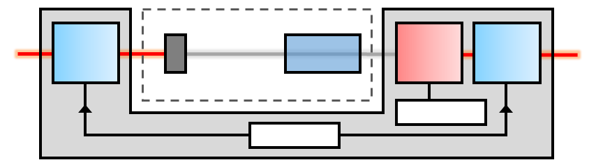
Figure 8: (color online) Fully attenuating transmission line (enclosed by dashed line) with limited-direct UQEC applied as a communication protocol to recover the input state. Transmission line definitions match those in Fig.7, and the UQEC notation is that of Fig.4. The large light-gray region is a sealed box indicating that the results of which operators are applied do not leave the box. Just after the VNDF, a particular result is $\lambda_{j}|0\rangle\langle 0|$, where $\lambda_{j}\equiv\langle e_{j}|\rho|e_{j}\rangle$ is a scalar. Thus only vacuum exists within the transmission line, but the recovery and decoding still recover $\rho$, if true projectors are used.

Thus, using UQEC as a communication protocol, if we use the paradigm of sending many identically prepared systems in the same state, then the party on the receiving side can tomographically measure $\rho$, regardless of how noisy the transmission line is.

The message sent can be encoded into $\rho$ by some pre-agreed method, such as chopping up its scalars into accurately discernible intervals and assigning letter values to each (see Sec.V for more details about this). The states sent could also each last for a certain time period, and series of states can be sent in a cycle. The method of message encoding is trivial. The amazing thing here is that we may not even need a transmission line at all!

This last observation comes from the fact that we assumed total absorption prior to the transmission line and were still able to treat it as a correctable error channel. If true, some of the startling implications of this are:

• No transmission lines are needed, and the encoded state can be into a perfect absorber (see (36)).

• Messages can be sent as states across any distance.

• There is no classical transmission signal.

• Messages can be received faster than a classical signal can send them. (See Sec.III.7 for why this does not violate special relativity, but still permits effective superluminal communication.)

• Alignment is irrelevant; relative position of sender and receiver is irrelevant because all information about the input state is encoded in subsystem-independent scalars $\lambda_{j}$.

• Messages cannot be classically eavesdropped, since the sender’s output is always vacuum.

• Messages cannot be corrupted or faked by interference in transit, since any mid-transit operation is lumped with the total error and corrected.

In the next few sections, we discuss the application of the above hypothetical implications, including how to realize them and why we should even consider them, given that they seem to contradict known physics.

As we will discuss in Sec.IV and the Conclusions, all of these seemingly impossible implications depend on the existence of true projection operations. Thus throughout Sec.III, we suppose that true projectors are possible, and then use the extraordinary consequences of that supposition to suggest a “no-projector theorem” in Sec.IV.

III.2 Design of an Ansible

The term ansible was coined by science fiction author Ursula K. Le Guin to describe any device capable of superluminal communication, an idea dating back to at least Isaac Asimov’s “hyper-wave relay.” While these were just plot devices, they happen to describe the application of teleporting unassisted QEC (UQEC) as a communication device with enforced total absorption.

The implementation of an ansible is simple: two separate devices called ansible halves (sender and receiver) are prepared in such a way that they enforce the index-linking of encoders $\{L_{j}\}$ and decoders $\{L_{j}^{{\dagger}}\}$ without any communication between them (basically cutting the light-gray-box connection in Fig.8). A general receiver also contains recovery operators $\{R_{q}\}$, and both ansible halves must apply their operators with equal probability. The information about which operators are applied must be kept inside the ansible halves in the classical sense, meaning that availability of this information is acceptable as long as users do not learn the outcomes. Figure 9 illustrates how this might be achieved. (Later, in Sec.V we will see that the recovery operators can be omitted if proper steps are taken, but for now we keep them to highlight the ansible’s origin as UQEC.)

The index linking of $\{L_{j},L_{j}^{{\dagger}}\}$ may be achieved by using a single true random number generator (TRNG) to generate and store the same random string of integers in each ansible half. This integer string must contain all the integers from each outcome at least once and in equal proportions. Internal clocks are synchronized to the factory clock, and thereafter are kept running. The clocks enforce the equal probability by selecting each index for an equal amount of time, while their synchronization enforces the index linking. The randomness of the index generation ensures that the outside world is ignorant about which pair $\{L_{j},L_{j}^{{\dagger}}\}$ is applied.

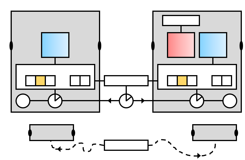
Figure 9: (color online) Preparation of a pair of ansible halves. (a) At the factory, a true random number generator (TRNG) generates an exhaustive random number sequence and writes it to an index memory in both halves, and no record of the sequence is retained externally. Internal clocks of the halves are synchronized to the factory clock so that they always point to the same index $j$ in both devices at the same time. Inertial trackers (IT) within the halves apply relativistic corrections to the clocks to keep them synchronized without need for communication between them. All notation is that of previous figures. (b) After the sequence is loaded into the halves, they are disconnected and travel away from the factory. Thus, a matched pair of ansible halves contains index-linked encoding and decoding operators $L_{j}$ and $L_{j}^{{\dagger}}$.

After the factory synchronizes the ansible halves, they are disconnected and go off in their separate directions. Both ansible halves contain inertial trackers (IT) which apply relativistic corrections to ensure that the clocks remain synchronized in spite of time-dilation effects. The reference frame of the factory is the reference that both devices treat as “correct.” For example, if the sender is moving away from the factory, its IT causes its clock to cycle faster to match the factory clock. If the receiver moves away from the factory at a different velocity, its IT adjusts its clock to run faster as well, again to match the factory clock. Thus, both ansible clocks remain synchronized without communicating with each other or with the factory. For this reason, the index-matching is not achieved through classical communication, but rather, through classical correlation.

Although the ansible halves could be operated with a line-of-sight pathway between them, perhaps by directing the output beam of the sender through a noisy fiber, as depicted in Fig.10a, we have already seen in (39) that the fiber and any noise channel, including full absorption can be grouped as one big correctable error channel, and thus, inserting a perfect absorber in the path as in Fig.10b does not change the output state, resulting in the effect of beam rebirth, which we will discuss shortly. Then, since only vacuum exists in the path, we can remove the fiber altogether and incorporate the absorber in the sender ansible half, as in Fig.10c. Thus, for these reasons, we see that Implications 1, 2, and 3 from Sec.III.1 are each reasonable in the context of such an ansible pair.

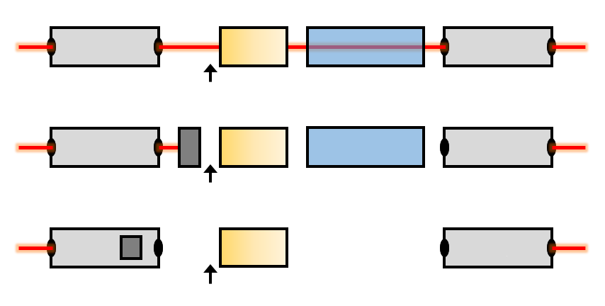
Figure 10: (color online) Operation of matched ansible halves. (a) A transmission path with an arbitrary error channel $\mathcal{E}$ and ideal fiber modeled as a phase shifter (PS). (b) Same transmission path with but with perfect absorber inserted (darkest rectangles). (c) Perfect absorber incorporated into the encoding ansible half, and the fiber removed completely. In each case, there is no classical communication between ansible halves, but rather each pair is classically correlated, due to their synchronized initialization at the factory as in Fig.9. See Sec.III.6 for a discussion of the strange prediction of the “beam rebirth” in (b) and (c). Arrows show the $j$th result at that point, where $\lambda_{j}\equiv\langle e_{j}|\rho|e_{j}\rangle$.

Implication 4 from Sec.III.1 is more troubling because it asserts the validity of superluminal communication. In part, this is due to Implication 2, which is valid because we could use a fiber/phase-shifter of any physical path length, and it would still be treated as part of a correctable error channel. Since the ansible halves can then be moved to any relative distance apart, they could easily be moved to a distance such that the time it takes to tomographically “read” the outupt state is much less than the time it would take a classical signal to send the same information. For example, if the ansible halves are moved $60$ light-minutes apart, but it only takes $1$ minute to tomographically measure a one-qubit message, then the message is learned by users of the ansible receiver $59$ minutes before the same message could reach them by radio. Section III.7 explains exactly how this is possible without violating special relativity.

The main reason this is even remotely plausible is the correlation of quantum operators in the ansible halves. The operators themselves are combinations of unitary gates and projectors, as shown in (17), and thus the fact that they are synchronized means that there is inherent nonlocality in the ansible pairs. This need not be entanglement; for example, quantum discord Ollivier and Zurek (2001); Henderson and Vedral (2001) includes quantum correlations beyond classical correlation that are not necessarily related to entanglement. Furthermore, the classical idea of state is inherently nonlocal, for example the solution to the heat equation has infinite propagation velocity. On the other hand, entanglement has been shown to have a lower-bound propagation speed of $10^{4}c$ Scarani et al. (2000); Gisin et al. (2000); Salart et al. (2008); Cocciaro et al. (2011); Yin et al. (2013), suggesting instantaneous correlation, as well. Thus, there are many natural mechanisms that can allow strong nonlocal correlations.

The idea of beam rebirth as seen in Fig.8 and Fig.10 is plausible because all of the information about the input state is reduced to the nonnegative scalars $\lambda_{j}$, and therefore it really makes no difference what the reference state $|\psi\rangle$ is between ansible halves. By including the perfect absorber in the design, we simply force the reference state to be initially vacuum, but any error channel can then change it to another state without affecting the correctability of the net error channel. Thus, as Implication 3 asserts, there is no standard concept of transmission signal here, and beam rebirth can be thought of as a kind of teleportation through localization-shifting of the wave function, caused by the built-in classical correlation of quantum operators. Section III.6 also explains that the recovery and encoding/decoding operators are generally active devices, supplying the energy necessary for beam rebirth from vacuum. Section V gives a detailed example explicitly showing how the computational basis interfaces to the vacuum.

Implication 5 that alignment is irrelevant is a powerful and important feature of this device. The reason for this is that the scalars $\lambda_{j}\equiv\langle e_{j}|\rho|e_{j}\rangle$, which contain all the information of the input state $\rho$, do not have any local dependence on a particular subsystem.

For example, suppose a mirror is placed just before the receiver in Fig.10c. The mirror acts as a beam splitter with device unitary $B_{\theta}\equiv e^{\theta(a_{1}^{{\dagger}}a_{2}-a_{1}a_{2}^{{\dagger}})}$ where $a_{1}$ and $a_{2}$ are annihilation operators, with $\theta=\frac{3\pi}{2}$ causing full reflectivity on its primary input so that $B_{\theta}a_{1}B_{\theta}^{{\dagger}}=a_{2}$ and $B_{\theta}a_{2}B_{\theta}^{{\dagger}}=-a_{1}$. For any state $\varsigma$ in its auxiliary input, it sends a version of $\varsigma$ to the main output, and redirects the primary input to the auxiliary output in a location other than the receiver’s input, as seen in Fig.11.

Recalling that $L_{j}=|\psi\rangle\langle e_{j}|$ where $\{|e_{j}\rangle\}$ are eigenstates of $\rho$, $R_{q}=|\psi\rangle\langle\phi_{q}|$ where $\{|\phi_{q}\rangle\}$ is a complete set of orthonormal states, and $\mathcal{A}_{0}(\rho)=|0\rangle\langle 0|\;\forall\rho$, then the particular results in Fig.11 just after the sender are

$$\begin{array}[]{*{20}l}{\mathcal{A}_{0}(L_{j}\rho L_{j}^{{\dagger}})}&\!\!{=\mathcal{A}_{0}(|\psi\rangle\langle e_{j}|\rho|e_{j}\rangle\langle\psi|)}\\ {}&\!\!{=\lambda_{j}\mathcal{A}_{0}(|\psi\rangle\langle\psi|)}\\ {}&\!\!{=\lambda_{j}|0\rangle\langle 0|.}\\ \end{array}$$ (40)

Next, apply an arbitrary error channel $\mathcal{E}$ with errors $E_{k}$, so that for any one of them, the result is

$$\rho_{(k,j)}^{\prime}\equiv E_{k}\mathcal{A}_{0}(L_{j}\rho L_{j}^{{\dagger}})E_{k}^{{\dagger}}=\lambda_{j}E_{k}|0\rangle\langle 0|E_{k}^{{\dagger}}.$$ (41)

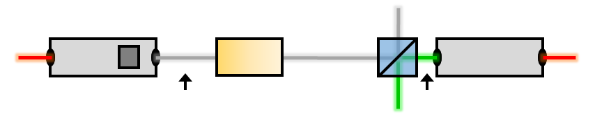
Figure 11: (color online) Ansible halves with a mirror modeled as a fully reflective beam splitter $B_{3\pi/2}$ just prior to the receiver. The notation is the same as in Fig.10c, except that here a gray line indicates the intermediate “beam” starting as the vacuum-proportional result just after the sender. The mirror sends intermediate result $\rho_{(k,j)}^{\prime}$ given in (41) away from the receiver, and sends some completely unrelated state $\widetilde{\varsigma}$ defined in (42) into the receiver instead. As (47) shows, the proper state $\rho$ is still recovered at the end. This proves Implication 5, that alignment of the ansible halves is irrelevant.

Then the mirror acts, modeled as a fully reflecting beam splitter with arbitrary state $\varsigma$ as auxiliary input, yielding

$$B_{{\textstyle{3\pi\over 2}}}(\rho_{(k,j)}^{\prime}\otimes\varsigma)B_{{\textstyle{3\pi\over 2}}}^{{\dagger}}=\widetilde{\varsigma}\otimes\rho_{(k,j)}^{\prime},$$ (42)

where $\widetilde{\varsigma}\equiv\sum\nolimits_{y,z=0,0}^{\infty,\infty}{{(-1)^{y+z}\varsigma_{y,z}|y\rangle\langle z|}}$, and $\varsigma_{y,z}\!\equiv\!\langle y|\varsigma|z\rangle$. Meanwhile, the correction procedure still continues on subsystem 1, with a given recovery operator producing

$$R_{q}\widetilde{\varsigma}R_{q}^{{\dagger}}\otimes\rho_{(k,j)}^{\prime}=\langle\phi_{q}|\widetilde{\varsigma}|\phi_{q}\rangle|\psi\rangle\langle\psi|\otimes\rho_{(k,j)}^{\prime}.$$ (43)

Then the $j$th decoder acts, and abbreviating the result as $\sigma_{(q,k,j)}\equiv L_{j}^{{\dagger}}R_{q}\widetilde{\varsigma}R_{q}^{{\dagger}}L_{j}\otimes\rho_{(k,j)}^{\prime}$, yields

$$\begin{array}[]{*{20}l}{\sigma_{(q,k,j)}}&\!\!{\!=\!\langle\phi_{q}|\widetilde{\varsigma}|\phi_{q}\rangle|e_{j}\rangle\langle\psi|\psi\rangle\langle\psi|\psi\rangle\langle e_{j}|\otimes\rho_{(k,j)}^{\prime}}\\ {}&\!\!{\!=\!\langle\phi_{q}|\widetilde{\varsigma}|\phi_{q}\rangle|e_{j}\rangle\langle e_{j}|\otimes\rho_{(k,j)}^{\prime}}.\\ \end{array}$$ (44)

Putting $\rho_{(k,j)}^{\prime}$ from (41) into (44) gives

$$\sigma_{(q,k,j)}\!=\!\lambda_{j}\langle\phi_{q}|\widetilde{\varsigma}|\phi_{q}\rangle|e_{j}\rangle\langle e_{j}|\otimes E_{k}|0\rangle\langle 0|E_{k}^{{\dagger}},$$ (45)

and then, since the user operating the receiver will be performing tomography on subsystem 1, we trace over subsystem 2, which gives

$$\begin{array}[]{*{20}l}{\text{tr}_{2}(\sigma_{(q,k,j)})}&\!\!{\!=\!\lambda_{j}\langle\phi_{q}|\widetilde{\varsigma}|\phi_{q}\rangle|e_{j}\rangle\!\langle e_{j}|\text{tr}(E_{k}|0\rangle\!\langle 0|E_{k}^{{\dagger}})}\\ {}&\!\!{\!=\!\lambda_{j}\langle\phi_{q}|\widetilde{\varsigma}|\phi_{q}\rangle|e_{j}\rangle\!\langle e_{j}|\langle 0|E_{k}^{{\dagger}}E_{k}|0\rangle.}\\ \end{array}\!\!$$ (46)

Finally, since the user does not know anything about which operators were applied, and since the ansible halves enforce the index linking of their encoder/decoder pairs, then the receiver’s output state is

$${\sum\nolimits_{q,k,j}\!{\text{tr}_{2}(\sigma_{(q,k,j)})}}=\sum\nolimits_{j}\!{\lambda_{j}|e_{j}\rangle\langle e_{j}|}=\rho,$$ (47)

where we used the facts that $\sum\nolimits_{q}{\langle\phi_{q}|\widetilde{\varsigma}|\phi_{q}\rangle}=\text{tr}(\widetilde{\varsigma})=1$ and $\sum\nolimits_{k}{E_{k}^{{\dagger}}E_{k}}=I$.

Thus, we see that the receiver user does obtain the original state $\rho$, regardless of the fact that we inserted a mirror which sent the intermediate state to a different subsystem than that to which the receiver ansible half was applied! Furthermore, the auxiliary input state $\varsigma$ is completely arbitrary and does not affect the result. Also, though we used a perfect mirror for a simple example, if it had been the mirror with phase shift such as what happened to $\varsigma$, the result would have been to simply add another error channel, which would get lumped with $\mathcal{E}$. The conclusion is that of Implication 5: alignment of the ansible halves is unimportant, and the preceding derivation supports the assertion that the scalar nature of the encoded state is the reason that this is possible.

Note that the preceding proof can be used as an alternative to the NRQT proof in Sec.II.5, the difference being that here, the noise was local, and we explicitly used a mirror to prove that alignment does not matter.

Also, this proof treats directly transmitted modes as the same mode to simplify labeling, whereas Sec.II.5 explicitly gives the sender and receiver their own modes; this is analogous to using one mode to describe a phase shifter instead of two modes as in App.C. The reason for using the single-mode transmission here is to highlight the action of the mirror to prove alignment irrelevance.

On a practical note, the “ansible” we have described thus far is only a one-way communication device. For full two-way communication, ansibles would need to be manufactured in crossed pairs, so that each two-way anisble half would contain a sending half and a receiving half of two separate one-way ansible pairs, as shown in Fig.12.

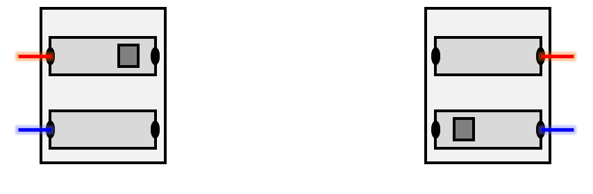
Figure 12: (color online) Two-way ansible. Alice sends a message as $\rho$ into sender $1$, which comes out as $\rho$ from Bob’s receiver $1$. Bob uses tomography and obtains Alice’s message from $\rho$ and then sends his response as $\rho^{\prime}$ into sender $2$, and it comes out as $\rho^{\prime}$ from Alice’s receiver $2$, where she can obtain Bob’s message from $\rho^{\prime}$ through tomography.

Now that we have described the realization of an ansible as a possible application of UQEC (supposing the possibility of true projectors), we are ready to examine some of its encryption properties.

III.3 Strong Encryption Between Ansible Halves

As described in Sec.III.2, operation of an ansible can be done without need of any broadcast signal or even a transmission line or alignment. Here, we discuss the encryption properties of this hypothetical technology.

In Fig.10c, we see that a message can be sent as a state that is proportional to the vacuum state in the region between ansible halves. Therefore the state “sent out” by the sender is always the vacuum, which means that no information about $\rho$ can be learned by attempting to perform tomography between the ansible halves.

The “sent state” may not remain vacuum, since any error channel may act along the way, but since those states have nothing to do with the input $\rho$, they do not permit $\rho$ to be learned either.

To test this, imagine that the auxiliary output of the beam splitter in Fig.11 is intercepted by an eavesdropper. What state will they get? The joint-system outcomes at that point are given in (44) and (45), and so the state available to the eavesdropper is

$${\sum\nolimits_{q,k,j}{\text{tr}_{1}(\sigma_{(q,k,j)})}}=\sum\nolimits_{k}{E_{k}|0\rangle\langle 0|E_{k}^{{\dagger}}},$$ (48)

which is simply error-corrupted vacuum $\mathcal{E}(|0\rangle\langle 0|)$, containing no information about the message $\rho$.

What if the eavesdropper uses recovery and decoding operators? In that case, the recovery operators are definitely independent because those can be generated instantaneously within each ansible half, so the eavesdropper can at best have index-independent set $\{R_{s}\}$. Furthermore, since the random-number strings and clock phase are unknown to the eavesdropper, their decoding operators will also be index-independent such as $\{L_{h}\}$. Thus, defining the eavesdropper’s possible outcomes as $\eta_{(q,k,j,h,s)}\equiv(I\otimes L_{h}^{{\dagger}}R_{s})\sigma_{(q,k,j)}(I\otimes R_{s}^{{\dagger}}L_{h})$, they get

$$\frac{{\sum\nolimits_{q,k,j,h,s}{\text{tr}_{1}(\eta_{(q,k,j,h,s)})}}}{{\text{tr}(\sum\nolimits_{q,k,j,h,s}{\text{tr}_{1}(\eta_{(q,k,j,h,s)})})}}={\textstyle{1\over n}}I,$$ (49)

which is the maximally mixed state, also containing no information about $\rho$.

However, there is one case in which the eavesdropper could be successful: if they guess or obtain the clock phase and the exact internal random-number string of the ansible pair, and maintain inertially tracked corrections from the creation point at the factory, then the eavesdropper’s decoding operators would be index-linked with those of the ansible such that their outcomes would be $\eta_{(q,k,j,j,s)}\equiv(I\!\otimes L_{j}^{{\dagger}}R_{s})\sigma_{(q,k,j)}(I\!\otimes R_{s}^{{\dagger}}L_{j})$, which sum to

$$\sum\nolimits_{q,k,j,s}{\eta_{(q,k,j,j,s)}}=\sum\nolimits_{j}{\lambda_{j}}|e_{j}\rangle\langle e_{j}|\otimes|e_{j}\rangle\langle e_{j}|,$$ (50)

and the state obtained by the eavesdropper is

$${\text{tr}_{1}(\sum\nolimits_{q,k,j,s}{\eta_{(q,k,j,j,s)}})}=\rho,$$ (51)

which is exactly the state obtained by the ansible receiver. Worse than that, this is done silently, since the receiver can detect no effect of this eavesdropping.

While it is highly unlikely that such eavesdropping could be accomplished by guessing or searching due to the high degree of synchronization required, it can be made far less likely by lengthening the random-number strings stored in the ansible pair, such that all numbers still occur an equal number of times. In that way, the probability of successful eavesdropping by luck or trial-and-error can be made arbitrarily close to zero by increasing the stored random-number string length.

Thus, Implication 6 from Sec.III.1 is mainly justified since eavesdropping the vacuum or any error-distorted version of it yields no information about the input state, with the caveat that the unpredictability of the internal random numbers needs to be as strong as possible.

Similarly, Implication 7 from Sec.III.1 is justified because any operation performed between the ansible halves is merely treated as another error channel, completely corrected away by the receiver. The caveat here is that the internal workings of the sender and receiver ansible halves must be protected from tampering; the error resistance only holds true between the ansible halves.

Of course, placing a spy at the receiver also circumvents the secure connection, but that is true for all security protocols. However, as long as some method of user authentication is employed, then the message is safe. Note that authentication requires a two-way ansible.

Thus, we can say that the ansible provides a strongly encrypted pathway for communication, because messages cannot be altered or easily eavesdropped in transit.

III.4 Quantum Broadcasting

The suggested possibility for successful eavesdropping of an ansible pair in Sec.III.3 can actually be used intentionally to enable multi-party communication, which we might call quantum broadcasting.

This can easily be seen from the joint-system state in (50), from which both parties will perceive the same state $\rho$ in their respective subsystems.

This broadcasting can be achieved by preparing multiple receiver ansible “halves” at the factory, in the same way as described in Fig.9, such that all receivers contain the same random number string, and all clocks are synchronized and maintained via internal inertial trackers. In the case of $N$ subsystems with matched receivers, the joint-system output state is

$$\eta\equiv\sum\nolimits_{j}{\lambda_{j}}|e_{j}^{(1)}\rangle\langle e_{j}^{(1)}|\otimes\cdots\otimes|e_{j}^{(N)}\rangle\langle e_{j}^{(N)}|,$$ (52)

where parenthetical superscripts are subsystem labels. The reduction for each subsystem, tracing over the other $N-1$ subsystems, is always $\rho$.

Thus, we can achieve quantum broadcasting since a single input state $\rho$ can be simultaneously sent to all parties possessing the receivers index-matched to the sender. An added advantage of this system is that if any one of the receivers breaks, the others keep receiving.

III.5 Effective Quantum Cloning

The quantum broadcasting application of Sec.III.4 is suggestively similar to quantum cloning. However, it is not quantum cloning because the joint-system state $\eta$ is not a tensor product of identical states, even though each reduction is the identical state $\rho$. For true quantum cloning, the joint output state would need to be $\rho^{\otimes N}\equiv\rho^{(1)}\otimes\cdots\otimes\rho^{(N)}$. Furthermore, limited-direct UQEC limits the family of states $\rho$ to those sharing the same set of eigenstates, while ideal quantum cloning would have no such limitation. Similarly, in insulating UQEC, though it can handle and transmit all possible states, the reductions would be in the form of the insulated state $\rho_{D}$, which is merely isomorphic to $\rho$.

However, although the joint output state is not $\rho^{\otimes N}$, we might nevertheless refer to the scenario where all the output reductions are $\rho$ as effective quantum cloning, and it may prove to be useful.

Note that the “no-cloning” theorem Wooters and Zurek (1982); Dieks (1982) only applies to unitary operations, and therefore in the context of more general quantum operations, such as QEC, the no-cloning theorem is generally not valid.

III.6 Wireless Power Transfer?

While scenarios such as Fig.10c make it appear as if a beam (and all its energy) is disappearing in one location and reappearing in another location, carrying with it some nonzero mean particle number and thus power, there is actually no power transfer.

The reason no power is transfered is that, as seen in (50), the input state’s ability to be effectively quantum-cloned means that energy is not conserved in the broadcasting process, even in the case of just one receiver.

This nonconservation of energy is perfectly explainable: the recovery/decoding process is an active process, meaning that it pumps energy into the system from the power used to operate the ansible receiver.

But how can the recovery/decoding operators be active devices if we showed in Sec.II.4.3 that they are combinations of projective filters and unitary gates? The answer is that unitary operations can be active power sources.

For example, consider the unitary vacuum displacement operator, $D(\alpha)\equiv e^{\alpha a^{{\dagger}}-\alpha^{*}a}$, where $a$ is the annihilation operator and $\alpha$ is a complex number, such that

$$|\alpha\rangle=D(\alpha)|0\rangle,$$ (53)

where $|\alpha\rangle$ is a coherent state of mean particle number $|\alpha|^{2}$. Since the input state is vacuum, with mean particle number $0$, then $D(\alpha)$ is an active unitary operator since it transforms the vacuum to a new state with a generally larger mean particle number.

To see how this relates to the ansible, the possible results after applying the recovery operator are

$$R_{q}E_{k}L_{j}\rho L_{j}^{{\dagger}}E_{k}^{{\dagger}}R_{q}^{{\dagger}}=\lambda_{j}|\langle\phi_{q}|E_{k}|\psi\rangle|^{2}|\psi\rangle\langle\psi|,$$ (54)

where everything is as defined in Sec.II.

Now suppose that we use vacuum as the reference state, setting $|\psi\rangle\equiv|0\rangle$. In that case, each possible result in (54) is proportional to the vacuum as

$$R_{q}E_{k}L_{j}\rho L_{j}^{{\dagger}}E_{k}^{{\dagger}}R_{q}^{{\dagger}}=\lambda_{j}|\langle\phi_{q}|E_{k}|0\rangle|^{2}|0\rangle\langle 0|,$$ (55)

from which we see that each result has mean particle number $0$, the same value we would get for the normalized sum of all results.

However, applying the decoder to (55) yields

$$L_{j}^{{\dagger}}R_{q}E_{k}L_{j}\rho L_{j}^{{\dagger}}E_{k}^{{\dagger}}R_{q}^{{\dagger}}L_{j}=\lambda_{j}|\langle\phi_{q}|E_{k}|0\rangle|^{2}|e_{j}\rangle\langle e_{j}|,$$ (56)

and since each state $|e_{j}\rangle\langle e_{j}|$ has nonzero mean particle number, and the same for the total state, then the mean particle number has been increased by the decoders.

Therefore, in this example, the decoders raise the vacuum to various other states of larger mean particle number, which proves that the decoders $L_{j}^{{\dagger}}$ are injecting energy into the output system. Specifically, recalling the operator implementation of Sec.II.4.3, since the projective part of $L_{j}^{{\dagger}}$ only incurs loss, then it is the unitary part of $L_{j}^{{\dagger}}$ that is responsible for injecting the power.

Thus, globally, energy is conserved in the ansible because the unitary operators used to realize the recovery and decoding operators are generally active devices which provide the energy to create the output beams.

That means that although the power outputs of the receivers do indeed mimic the input power of the sender, the actual power of each output beam would come from the receiver’s local power source, thereby making this device incapable of power transfer.

III.7 Effective Superluminal Communication Without Violating Special Relativity

Strictly speaking, the ideal ansible of Sec.III.2 is not capable of superluminal (faster-than-light) communication, because it would technically take an infinite number of measurements to perform perfect tomography, even assuming all equipment is ideal. Therefore, special relativity is not violated by the ansible, because in theory, it cannot send a perfect message in a finite time.

However, for communication purposes, we merely need to measure the state to within some acceptable tolerance, and typically that can be done very well using unbiased estimators for which the mean of the estimator is the quantity sought, and the error can be made acceptably small for reasonable sample times.

Furthermore, the classical correlations involved have theoretically infinite propagation velocity, which is acceptable since they do not carry classical information by themselves. Thus, the inherent nonlocality of the strongly-correlated ansible halves and the nonlocality of the scalars $\lambda_{j}$ are what make long-range superluminal correlation possible (supposing that true projectors are possible), and the acceptable approximation of finite samples of unbiased estimators in the receiver’s tomography is what makes effective superluminal communication possible without violating special relativity. Note that this is not the same thing as proposing superluminal communication with entanglement.

Now that we have discussed the ansible as if it were possible, recall that superluminal communication and quantum cloning are familiar indicators of impossible processes. Therefore we now propose a theorem that explains why the ansible is likely impossible.

IV Proposal of a “No-Projector Theorem”

To this point, all the abnormal effects related to the ansible, such as effective superluminal communication and effective quantum cloning, can be traced back to the supposition that we can implement a single true projector deterministically (see Sec.II.4.4 and App.B).

Although Sec.II.7 proposed a seemingly logical method of realizing true projectors, we will see in Sec.V that even that will fail since it does not allow one projector to be applied without the other. Therefore, we propose the following theorem:

No-Projector Theorem:  It is impossible to deterministically implement any operation consisting of only a projector such as $P\equiv|\psi\rangle\langle\psi|$, where $|\psi\rangle$ is a pure state, without postselection.

Notice that if we use $|\psi\rangle\langle\psi|$ to represent a pure state, there is no problem; the no-projector theorem only observes the impossibility of operations in the form of $|\psi\rangle\langle\psi|$. Furthermore, as we saw in Sec.II.7, it is quite possible to realize true projectors in the context of a Kraus-complete quantum operation, but that is different from deterministically producing a lone projector.

No-Subtraction-Operator Corollary:  It is impossible to deterministically implement the annihilation or subtraction operator, without postselection.

No-Operator-Superposition Corollary:  It is impossible to deterministically implement superposition of operators such as $cA+dB$, where $c$ and $d$ are complex scalars and $A$ and $B$ are operators, without postselection.

These corollaries allude to the amazing work on subtraction operators and operator superposition in Zavatta et al. (2009), which demonstrates postselected application of operator superposition such as $aa^{{\dagger}}-e^{i\phi}a^{{\dagger}}a=I$, where $a$ is the annihilation operator. It is easy to show that if postselection were not necessary, then these techniques could be used to implement true projectors. Therefore, the postselection is an important part of realizing projectors in these methods, and we will see that it allows us to emulate scalar zero, and that it is also the reason that classical communication must be involved.

Actually, the no-projector theorem and its corollaries above are all manifestations of a more general theorem; that it is impossible to implement any nonunitary rank-1 operation without postselection, where the rank of a quantum operation is the minimum number of Kraus operators it can have over all possible decompositions. However, since the polar decomposition allows any operator to be expressed as a product of a nonnegative Hermitian projector $P$ and a unitary operation $U$, then the problem can be simplified to the realization of projectors, though it is not limited to rank-1 projectors (in this case, rank is the number of nonzero eigenvalues of $P$).

A more general way to state the no-projector theorem would be: In an $n$-level quantum system, with complete orthonormal basis $\{|\phi_{k}\rangle\}$, no projector $P\equiv\sum\nolimits_{k=1}^{k\leq n}r_{k}|\phi_{k}\rangle\langle\phi_{k}|$, where $r_{k}$ are real nonnegative scalars, can be implemented as a rank-$1$ quantum operation, without postselection, unless $P=I$ is the identity (in which case it is unitary and not merely a projector).

To prove the no-projector theorem, first we will show that Kraus completeness is a necessary consequence of the completeness of the orthonormal basis of the environment for a joint system that yields some physical quantum operation. Then, using polar decomposition, we will see that all Kraus completeness statements can be written with projectors only. Then, the fact that the smallest nontrivial environment is a qubit will prove that there must always be at least two projectors for a nonunitary operation to obey Kraus completeness, which proves that no physical quantum operation can consist of fewer projectors than what is needed for Kraus completeness.

First, following Hedemann (2014), start with the identity-identity

$$I^{(S)}\otimes I^{(E)}=I,$$ (57)

for $n_{S}$-level system $S$ and $n_{E}$-level environment $E$. Then, expand $I^{(E)}$ with any complete orthonormal basis as $I^{(E)}=\sum\nolimits_{k=1}^{n_{E}}|\phi_{k}^{(E)}\rangle\langle\phi_{k}^{(E)}|$, so (57) becomes

$$\sum\limits_{k=1}^{n_{E}}(I^{(S)}\otimes|\phi_{k}^{(E)}\rangle)(I^{(S)}\otimes\langle\phi_{k}^{(E)}|)=I.$$ (58)

Then apply joint-system unitary $U^{{\dagger}}$ from the left and $U$ from the right and use $U^{{\dagger}}U=I$ to get

$$\sum\limits_{k=1}^{n_{E}}U^{{\dagger}}(I^{(S)}\otimes|\phi_{k}^{(E)}\rangle)(I^{(S)}\otimes\langle\phi_{k}^{(E)}|)U=I.$$ (59)

Then apply $(I^{(S)}\!\otimes\langle\psi_{0}^{(E)}|)$ from the left, $(I^{(S)}\!\otimes|\psi_{0}^{(E)}\rangle)$ from the right, and use $(I^{(S)}\!\otimes\langle\psi_{0}^{(E)}|)I(I^{(S)}\!\otimes|\psi_{0}^{(E)}\rangle)=$ $I^{(S)}\!\otimes\langle\psi_{0}^{(E)}|\psi_{0}^{(E)}\rangle=I^{(S)}$ on the right to get

$$\sum\limits_{k=1}^{n_{E}}E_{k}^{(S){\dagger}}E_{k}^{(S)}=I^{(S)},$$ (60)

which is a Kraus-completeness relation where $E_{k}^{(S)}\equiv$ $(I^{(S)}\otimes\langle\phi_{k}^{(E)}|)U(I^{(S)}\otimes|\psi_{0}^{(E)}\rangle)$ are the Kraus operators. Thus, since (60) was derived from the completeness of the basis spanning $E$, that means Kraus completeness is a direct consequence of the completeness of the basis of $E$. Although these $E_{k}^{(S)}$ imply a joint system starting in product form as $\rho^{(S)}\otimes|\psi_{0}^{(E)}\rangle\langle\psi_{0}^{(E)}|$, it also applies to a mixed initial environment, which just means more Kraus operators, and a generally correlated initial joint system, since that can always be converted to product form by inserting a preliminary quantum operation converting a general product of states to the correlated state, resulting in more Kraus operators again.

To see that only projectors really matter, recall that all operators $\Omega$ have a right-polar decomposition $\Omega=UP$ where $U\equiv WV^{{\dagger}}$ is unitary, $P\equiv\sqrt{\Omega^{{\dagger}}\Omega}=V\Sigma V^{{\dagger}}$ is nonnegative Hermitian, where $\Omega=W\Sigma V^{{\dagger}}$ is the singular-value decomposition (SVD) of $\Omega$ where $W$ and $V$ are unitary and $\Sigma$ is the nonnegative diagonal matrix of singular values of $\Omega$. Therefore, all Kraus operators can be decomposed as (omitting $S$ labels on the right),

$$E_{k}^{(S)}=U_{k}P_{k},$$ (61)

and then putting this into (60) gives

$$\sum\limits_{k=1}^{n_{E}}(U_{k}P_{k})^{{\dagger}}U_{k}P_{k}=\sum\limits_{k=1}^{n_{E}}P_{k}^{{\dagger}}U_{k}^{{\dagger}}U_{k}P_{k}=\sum\limits_{k=1}^{n_{E}}P_{k}^{{\dagger}}P_{k}=I^{(S)},$$ (62)

which shows that the only thing that really ever matters about Kraus completeness is the projectors in this “projective Kraus completeness” relation in (62) (left unsimplified to highlight its relation to Kraus completeness), where the $P_{k}=V_{k}\Sigma_{k}V_{k}^{{\dagger}}$ are general weighted projectors of form $P_{k}=\sum\nolimits_{m=1}^{m\leq n}r_{k|m}|\phi_{k|m}\rangle\langle\phi_{k|m}|$ where $r_{k|m}\!=\!(\Sigma_{k})_{m,m}\!\geq\!0$ and $|\phi_{k|m}\rangle$ is the $m$th column vector of $V_{k}$, both from the SVD of $E_{k}$. Thus, we have proven that projective Kraus completeness is also a necessary consequence of the completeness of the environmentbasis.

Finally, since the smallest nontrivial environment has $\min(n_{E})=2$ levels, (62) shows that there must always be at least two projectors in any physical nonunitary quantum operation to maintain the necessary projective Kraus completeness. Thus we have proven the no-projector theorem up to postselection, and we get another corollary:

No-Kraus-Undercompleteness Corollary:   A quantum operation $\mathcal{E}(\rho)\equiv\sum\nolimits_{k}E_{k}\rho E_{k}^{{\dagger}}$ is physical iff it is Kraus complete $\sum\nolimits_{k}E_{k}^{{\dagger}}E_{k}=I$ on the full Hilbert space of $\mathcal{E}(\rho),\;\forall\rho$.

The reason that postselection allows “deterministic” rank-1 nonunitary operations is that by performing a measurement and looking at the result to do the postselection, our reality becomes defined by a particular result(s) of the mixture, which can have a support that is less-than-complete on the original full space. This permits a “Kraus-undercompleteness” to be considered complete within a particular result of a mixture. The price we pay is the fundamental unpredictability of the postselection events, which causes increased wait times and the need to communicate the postselection results.

For example, consider a detector with a complete set of projective measurement operators $\Pi_{j}$ such that $\Sigma_{j}\Pi_{j}^{{\dagger}}\Pi_{j}=I$. Then, the Kraus operators for the full event (evolution by $U$, detection, reduction) are $E_{k|j}^{(S)}\equiv$ $(I^{(S)}\otimes\langle\phi_{k}^{(E)}|)\Pi_{j}U(I^{(S)}\otimes|\psi_{0}^{(E)}\rangle)$ for the $j$th detection result. Then, supposing the simplest case of measurement operators with form $\Pi_{j}=I^{(S)}\otimes|\phi_{j}^{(E)}\rangle\langle\phi_{j}^{(E)}|$, the Kraus operators are

$$E_{k|j}^{(S)}=\delta_{j,k}(I^{(S)}\otimes\langle\phi_{j}^{(E)}|)U(I^{(S)}\otimes|\psi_{0}^{(E)}\rangle),$$ (63)

so that given that a particular detection output happens, the projective Kraus completeness gets truncated to

$$\sum\limits_{k=1}^{n_{E}}P_{k|j}^{{\dagger}}P_{k|j}=P_{j}^{{\dagger}}P_{j}<I^{(S)}$$ (64)

which shows how postselection can cause apparent Kraus undercompleteness. By interacting with the detector, we are “along for the ride” on the particluar reality of just one of its measurement operators. The price we pay for this is that the postselection detection acts like an absorptive projective filter, inducing a mixture with the vacuum, and causing the instant of detection to be fundamentally uncertain.

We now go through a step-by-step example of how an ansible would function, and in the process we show why a true ansible would not work, but also find a way to make a pseudo-ansible; a device for connection-free noise-resistant light-speed communication.

V How To Build a Pseudo-Ansible

Here we begin by first returning to the supposition that true projectors and therefore true ansibles are possible. We then find a flaw and use it to develop the idea of pseudo-ansibles. The general setup is shown in Fig.13.

Figure 13: (color online) Overview of general one-way ansible protocol. The middle stage is general transmission modeled as noise channel $\mathcal{E}$, which can be any noise, even the complete attenuation channel from Sec.III.1.

In the following sections, we will discuss the details of each of the stages shown in Fig.13. In keeping with previous convention, here we use $\{|\widetilde{1}\rangle,|\widetilde{2}\rangle,\ldots\}$ as the computational basis to distinguish it from the Fock basis.

V.1 Message Preparation

Following Sec.II.8, we will use insulating UQEC to send our message, allowing us to restrict input to pure states, ensuring only superposition scalars are involved. For one qubit, this means we only have two degrees of freedom for information storage.

One way to store this information is to use spherical parameterization, and chop up each parameter by the number of letters in our alphabet, limited only by resolution accuracy of measurement.

For example, a single-qubit message state has the form

$$|\xi\rangle\equiv c_{\theta}|\widetilde{1}\rangle+s_{\theta}e^{i\phi}|\widetilde{2}\rangle,$$ (65)

where $c_{\theta}\equiv\cos(\theta)$, $s_{\theta}\equiv\sin(\theta)$, where $\theta\in[0,{\textstyle{\pi\over 2}}]$ and $\phi\in[0,2\pi)$. Supposing we could accurately chop these parameters each into, say, $M=41$ pieces, to fit 26 letters, 10 numbers, a period, a question mark, a space “$\_\,$”, “$\sim$”, and “$\ast$” in that order, where “$\sim$” means “no message” and “$\ast$” means “start new message,” then in the range of $[0,1]$, the $m$th character $\chi_{m}$ of this alphabet would have value $\chi_{m}={\textstyle{{2m-1}\over{2M}}}$, where $m=\{1,\ldots,M\}$. Then let $\theta\equiv{\textstyle{\pi\over 2}}\chi_{m}$ for character one, and $\phi\equiv 2\pi\chi_{m}$ for character two. To send a message consisting of any two characters, such as “GO,” we simply set $\theta\equiv{\textstyle{\pi\over 2}}\chi_{7}\approx 0.249[\text{rad}]$ and $\phi\equiv 2\pi\chi_{15}\approx 2.222[\text{rad}]$. Thus, the message state is

$$\rho=|\xi\rangle\langle\xi|\approx\left({\begin{array}[]{*{20}l}{0.939}&{0.239e^{-i2.222}}\\ {0.239e^{i2.222}}&{0.061}\\ \end{array}}\right)\!.$$ (66)

Typically, there is some fiduciary state $|\xi_{0}\rangle$ naturally produced by our single-photon source (SPS), and we must use $\theta$ and $\phi$ to apply $U=\epsilon_{|\xi\rangle}\epsilon_{|\xi_{0}\rangle}^{{\dagger}}$ as the particular unitary that transforms $|\xi_{0}\rangle$ to message $|\xi\rangle$, where $\epsilon_{|A\rangle}$ is the eigenvector matrix of $|A\rangle\langle A|$.

V.2 Ansible Sender: Encoding and Vacuum Conversion

Here we examine two different methods of encoding, both of which use conversion to vacuum for connection-free communication and full noise resistance.

V.2.1 Time-Bin Projector Method

As in Sec.II.7, if the input photon’s momentum qubit has state $|\widetilde{1}\rangle$, our joint-system input state is $\rho\otimes|\widetilde{1}\rangle\langle\widetilde{1}|$. Then, recalling the insulating-UQEC encoding operators $D_{j}=P_{|\widetilde{1}\rangle}\epsilon_{|D_{j}\rangle}^{{\dagger}}$, only applying the unitary part of this as $|\xi_{j}\rangle\equiv\epsilon_{|D_{j}\rangle}^{{\dagger}}|\xi\rangle$ gives $\rho_{j}\otimes|\widetilde{1}\rangle\langle\widetilde{1}|$, analogous to the input of Fig.6, where $\rho_{j}\equiv|\xi_{j}\rangle\langle\xi_{j}|$. Then, the application of the time-separated projector channel of Sec.II.7 yields

$$\rho_{j}^{\prime}\equiv(\rho_{j})_{1,1}|1_{\tau_{1}},0_{\tau_{2}}\rangle\langle 1_{\tau_{1}},0_{\tau_{2}}|+(\rho_{j})_{2,2}|0_{\tau_{1}},1_{\tau_{2}}\rangle\langle 0_{\tau_{1}},1_{\tau_{2}}|,$$ (67)

where $\rho_{j}^{\prime}\equiv(\rho_{j})_{\text{CNOT}}$, $(\rho_{j})_{a,b}\equiv\langle\widetilde{a}|\rho_{j}|\widetilde{b}\rangle$, and $\tau_{k}$ labels time-bin $k$. From (128), we recognize the scalars in (67) as $(\rho_{j})_{1,1}=d_{j}$ and $(\rho_{j})_{2,2}=1-d_{j}$, so that (67) becomes

$$\rho_{j}^{\prime}\equiv d_{j}|1_{\tau_{1}},0_{\tau_{2}}\rangle\langle 1_{\tau_{1}},0_{\tau_{2}}|+(1-d_{j})|0_{\tau_{1}},1_{\tau_{2}}\rangle\langle 0_{\tau_{1}},1_{\tau_{2}}|.$$ (68)

Now we are ready to expose the flaw of this projector method. First, though it seems like (68) is a step-function in time, which would separate its scalars in time, it is actually a true mixture over both time bins. This means that we only get a photon in one time bin and vacuum in the other, but never get a photon in each time bin or vacuum in both; a step function in time would yield a photon in both time bins, so that is not what (68) means.

If we just focus on $\tau_{1}$, then tracing over $\tau_{2}$ gives

$$\text{tr}_{\tau_{2}}(\rho_{j}^{\prime})=d_{j}|1_{\tau_{1}}\rangle\langle 1_{\tau_{1}}|+(1-d_{j})|0_{\tau_{1}}\rangle\langle 0_{\tau_{1}}|,$$ (69)

which is a mixture with vacuum with both results in $\tau_{1}$. Then, applying a total absorber $\mathcal{A}_{0}$ gives

$$\mathcal{A}_{0}(\text{tr}_{\tau_{2}}(\rho_{j}^{\prime}))\!=\!d_{j}|0_{\tau_{1}}\rangle\langle 0_{\tau_{1}}|\!+\!(1\!-\!d_{j})|0_{\tau_{1}}\rangle\langle 0_{\tau_{1}}|\!=\!|0_{\tau_{1}}\rangle\langle 0_{\tau_{1}}|,$$ (70)

so the information in the scalars is lost. Thus, focusing on either time bin does not yield the results we would expect from the application of a lone projector.

If we try to use the whole state, applying $\mathcal{A}_{0}$ gives

$$\begin{array}[]{*{20}l}{\mathcal{A}_{0}(\rho_{j}^{\prime})}&\!\!{=d_{j}|0_{\tau_{1}},\!0_{\tau_{2}}\rangle\langle 0_{\tau_{1}},\!0_{\tau_{2}}|\!+\!(1-d_{j})|0_{\tau_{1}},\!0_{\tau_{2}}\rangle\langle 0_{\tau_{1}},\!0_{\tau_{2}}|}\\ {}&\!\!{=|0_{\tau_{1}},\!0_{\tau_{2}}\rangle\langle 0_{\tau_{1}},\!0_{\tau_{2}}|,}\\ \end{array}$$ (71)

so again, the scalar information is lost.

Therefore, we have shown that implementing true projectors as part of a Kraus-complete channel yields the same type of vacuum mixtures as the application of an absorptive projector, thus preventing the ansible from achieving superluminal communication.

The reason it is easy to think that a time-bin projector channel would behave like a step function of projectors over time is because if true lone projectors were possible, then if we did implement a step function of them over time, choosing each one at random with equal probability and applying only one every two time bins, then an observer who chose a sample time at least two-time bins long but was ignorant of which projector was applied, would report the output to be in the state shown in (67). But applying a lone projector at a given instant in time is impossible because then we would be free to stop before applying the other, and the operation would not be Kraus complete and therefore not physical.

However, we can still get connection-free light-speed communication if we use postselection in the form of a detector that tells us which result of the mixture is happening, and therefore which scalar is active at that instant. This will require us to classically transmit the results of the postselection, but we can now abandon this time-bin projector method and just use detectors instead. This will lead to a more robust version of light-speed limited communication as will soon see.

V.2.2 Postselective Projector Method

Here, we bypass the time-bin projector method completely and return to a prepared state $\rho$ from (66) and (65). We still apply $\epsilon_{|D_{j}\rangle}^{{\dagger}}$ the unitary part of the encoders to get $\rho_{j}$ as in Sec.V.1, but now we simply apply a polarizer as the projector $P_{|\widetilde{1}\rangle}$ for that part of the encoding.

Since a polarizer is an absorptive projective filter (APF), its action on results $\rho_{j}$ yields (as in App.B)

$$P_{|\widetilde{1}\rangle}^{(\text{APF})}(\rho_{j})=d_{j}|1\rangle\langle 1|+(1-d_{j})|0\rangle\langle 0|,$$ (72)

where $d_{j}\!=\!(\rho_{j})_{1,1}$, and we have converted to the Fock basis and suppressed polarization.

Here we note that while total absorption would again conceal the scalars as in Sec.V.2.1 and (30), we can emulate a true projector by using postselection, effectively annihilating the vacuum and replacing it with a scalar zero without actually doing so.

Since we need an absorber anyway (to force vacuum, so we can eliminate the need for a quantum connection), we instead place a detector in the “output beam,” and we only recognize instances of a detector click as being part of the process, resulting in

$$\Pi_{\overline{0}}P_{|\widetilde{1}\rangle}^{(\text{APF})}(\rho_{j})\Pi_{\overline{0}}^{{\dagger}}=d_{j}|1\rangle\langle 1|,$$ (73)

where $\Pi_{\overline{0}}\equiv\sum\nolimits_{k=1}^{\infty}{|k\rangle\langle k|}$ is the nonvacuum measurement operator of an ideal on-off single-photon detector. Then, accounting for the fact that the detector absorbs the photon in the act of detecting it we apply $\mathcal{A}_{0}$ to get

$$(D_{j}\rho D_{j}^{{\dagger}})_{\text{PS}}^{(\text{APF})}\equiv\mathcal{A}_{0}(\Pi_{\overline{0}}P_{|\widetilde{1}\rangle}^{(\text{APF})}(\rho_{j})\Pi_{\overline{0}}^{{\dagger}})=d_{j}|0\rangle\langle 0|,$$ (74)

which are the desired results, where PS means “postselected,” since we looked at the measurement result. While it may seem like cheating to involve the detector’s projectors, we pay for it by interacting with the system, discarding unwanted results, and then having to communicate those results to the receiver. Thus, realizing a true projector via postselection imposes a light-speed limit.

In practice, since polarizers are not perfect, it may be better to use a polarizing beam splitter (PBS) and send one output beam to a detector and the other beam to a beam dump (BD), as in Fig.14b (BD not shown).

Also, there is no need to elongate the trial time as in the temporal purification methods mentioned in App.B. Here, we actually want the form of (72), and therefore we keep the trial time constant from input to output.

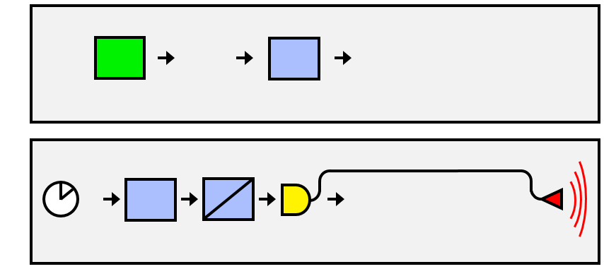
Figure 14: (color online) Schematic of total sender of a pseudo-ansible. (a) Message preparation. (b) Ansible sender, emitting a classical grouping signal (CGS) to communicate the postselection results. Details are given in the text. (Stored random-number strings are not shown.)

V.3 Ansible Receiver: Conversion to Single-Photon Basis and Decoding

An interesting property of the recovery operators $R_{q}\equiv|\psi\rangle\langle\phi_{q}|$ is that they form a “trace-and-replace” channel, meaning that whatever the input state is, it is traced-away and replaced by the reference state $|\psi\rangle$.

In terms of the receiver operations, this means that a single-photon source (SPS) effectively realizes the recovery and the projective part of the decoding operators.

The joint state of sender and receiver after encoding and postselection is

$$(D_{j}\rho D_{j}^{{\dagger}})_{\text{PS}}^{(\text{APF})}\otimes|1\rangle\langle 1|=d_{j}|0\rangle\langle 0|\otimes|1\rangle\langle 1|,$$ (75)

where $|1\rangle\langle 1|$ is the initial state of the receiver’s SPS output. If noise $\mathcal{E}$ acts on the sender’s output, we get

$$\eta_{j}=d_{j}\mathcal{E}(|0\rangle\langle 0|)\otimes|1\rangle\langle 1|,$$ (76)

where $\eta_{j}\equiv\mathcal{E}((D_{j}\rho D_{j}^{{\dagger}})_{\text{PS}}^{(\text{APF})})\otimes|1\rangle\langle 1|$. The receiver’s photon state is found by tracing over the sender as

$$\text{tr}_{1}(\eta_{j})=d_{j}|1\rangle\langle 1|.$$ (77)

Since this is already the pass-state for the true projective part of the decoding operator, we can omit that stage and directly apply the unitary part of the decoders as

$$\epsilon_{|D_{j}\rangle}\text{tr}_{1}(\eta_{j})\epsilon_{|D_{j}\rangle}^{{\dagger}}=d_{j}|D_{j}\rangle\langle D_{j}|,$$ (78)

where the matched indices are enforced by the factory synchronization of these operators with their counterparts in the sender and “discarding” trials in which the “no click” is reported by the classical grouping signal (we will discuss that more below).

Then, since the receiver does not keep track of which decoding unitaries are applied, tomography will find the system to be in the state (where $m_{n}\equiv n(2n-1)=6$)

$$\frac{\sum\nolimits_{j=1}^{m_{n}}\epsilon_{|D_{j}\rangle}\text{tr}_{1}(\eta_{j})\epsilon_{|D_{j}\rangle}^{{\dagger}}}{\text{tr}(\sum\nolimits_{j=1}^{m_{n}}\epsilon_{|D_{j}\rangle}\text{tr}_{1}(\eta_{j})\epsilon_{|D_{j}\rangle}^{{\dagger}})}={\textstyle{1\over{2n-1}}}\sum\limits_{j=1}^{m_{n}}{d_{j}|D_{j}\rangle\langle D_{j}|}=\rho_{D},$$ (79)

which is the insulated version of message $\rho$.

The classical grouping signal (CGS) is needed to determine which trials contain $d_{j}$ and which trials contain $1-d_{j}$. But we do not need to discard trials with $1-d_{j}$; we simply interpret their message state as a bit-flipped version of the intended message.

If both SPSs in sender and receiver are deterministic, meaning that photon emission can be controlled by classical pulses, then they can be synchronized by the inertial trackers, allowing for the time of CGS travel.

Thus, the tomography initially collects data during every trial, only marking results by local receiver time. Then, when the CGS arrives, the data, previously stored in classical memory, is then sorted into two groups corresponding to scalars $d_{j}$ and $1-d_{j}$. Amazingly, this means that the message transmission happens instantaneously, regardless of distance, but that no sense can be made out of the data until the CGS arrives.

Note that deterministic photon production has been achieved Wei et al. (2014), and since all operations we need can be kept within the same cryogenically cooled region, it will retain its ideal properties.

If the SPSs are not deterministic, the CGS information may need to either be transmitted as a very narrow pulse in time, or include information about the exact times the postselecting detector fired. The benefit of deterministic SPSs is that the CGS can just be a rectangular pulse train with a peak or trough filling each entire trial window. In either case, the tomographic clicks accepted as data must be coincidences with the preordained time of photon production or with a heralding photon from a nondeterministc SPS, and an inertial history of the receiver will be needed to match the events properly.

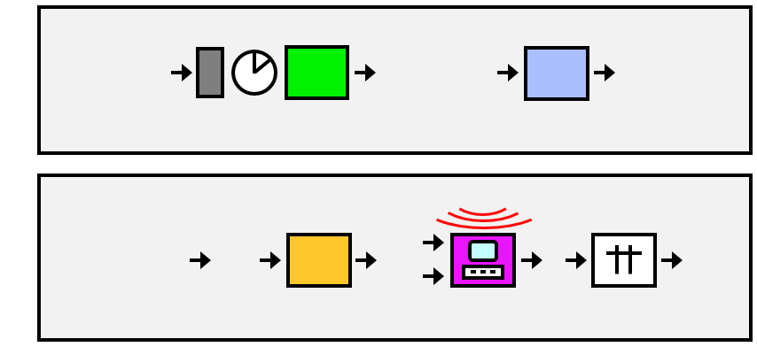
Figure 15: (coloronline)Schematicoftotalreceiver.(a)Pseudo-ansiblereceiver.(b)Tomography,extraction,reading. See the text for explanations.

V.4 Tomography, Extraction, and Message Reading

Here, we get an estimate of $\rho$ via state tomography on the receiver output, where only detections coincident to the time-frame-adjusted CGS are treated as data.

The tomography yields a numerical representation of $\rho_{D}$ from (79). Then, we perform extraction by computing

$$\rho=3\rho_{D}-I.$$ (80)

Next, we read the data from the extracted state $\rho$. In the scheme of Sec.V.1, the character-label integer is $m={\textstyle{1\over 2}}(2M\chi_{m}+1)$, and since the superposition character is $\chi_{m}={\textstyle{2\over\pi}}\cos^{-1}(\sqrt{\rho_{1,1}})\pm{\textstyle{1\over{2M}}}$, and the phase character is $\chi_{m}={\textstyle{1\over{2\pi}}}(\arg(\rho_{2,1})+2\pi\delta_{\text{sgn}(\arg(\rho_{2,1})),-1})\pm{\textstyle{1\over{2M}}}$ (which remaps the phase to $[0,2\pi)$ if arg outputs on $[-\pi,\pi)$ as for $\text{atan}2(y,x)$), then the character-label integers are given from the extracted state $\rho$ by

$$\begin{array}[]{*{20}l}{m_{\theta}}&\!\!{=\text{round}({\textstyle{{2M}\over\pi}}\cos^{-1}(\sqrt{\rho_{1,1}})+{\textstyle{1\over 2}})}\\ {m_{\phi}}&\!\!{=\text{round}({\textstyle{M\over{2\pi}}}\arg(\rho_{2,1})+M\delta_{\text{sgn}(\arg(\rho_{2,1})),-1}+{\textstyle{1\over 2}})}.\\ \end{array}$$ (81)

Treating (66) as the extracted $\rho$ (since that presentation was rounded, we can use it to simulate measurement error here), then putting it into (81) yields

$$\left.{\begin{array}[]{*{20}l}{m_{\theta}}&\!\!{=\text{round}(7.014)}&\!\!{=7}&\!\!{\to\text{``G''}}\\ {m_{\phi}}&\!\!{=\text{round}(14.999)}&\!\!{=15}&\!\!{\to\text{``O''}}\\ \end{array}}\right\}\to\text{``GO''},$$ (82)

where a look-up table of the character meanings was used to translate the message, successfully completing the one-way pseudo-ansible protocol, as depicted in Fig.15b.

Note that message preparation can be built into the sender, and tomography/extraction/message-reading can be built into the receiver, so that all their users have to do is type their messages in at one end, and read the message from a display screen at the other end.

VI Conclusions

This paper presented a theoretically justified proposition for noise-resistant quantum teleportation (NRQT) – a method of transporting a state between spatial modes while protecting it from any quantum noise channel that acts in the region between source and destination.

Section II gave an overview of unassisted quantum error correction (UQEC), which is the mechanism that enables protection of a quantum state against all noise channels, where the term unassisted means that no ancilla systems are necessary. In particular, UQEC does not need encoding or measurement ancillas.

It must be emphasized that UQEC is not practical for QEC. As explained in App.A, the term “unassisted” only applies in a theoretical sense because a true UQEC channel requires tracing over a larger system with an error-free subsystem, and though applying the UQEC channel classically in the local system is technically “unassisted,” its tomographic nature and the nonexistence of lone projectors from Sec.IV makes it impractical for quantum computation. Nevertheless, UQEC proved to be a valuable tool for investigating the existence of true projectors.

The fundamental principle of UQEC is that it reduces the input state to scalars which are not bound to any particular subsystem since scalars pass through Kronecker products. The index-synchronization of encoding and decoding operators allows the state to be rebuilt perfectly, even when some arbitrary error channel acts between them. When the rebuilding (decoding) happens in a different spatial mode than the encoding, we get a teleportation effect combined with the UQEC.

Section II.4 showed how to implement the UQEC quantum operations in a state-free manner, and used a classical realization of the channel that utilizes random numbers to enforce ignorance on the outside world, and to enable index-linking of the encoding and decoding operations over great distances without a connection. Since the communication protocol is tomographical at the receiving end, this classical realization does not affect the estimation of the state.

Then, Sec.II.4.3 showed that the Kraus operators needed require nonunitary operators such as projectors, and Sec.II.4.4 showed that absorptive projective filters (APFs) such as polarizers are not actually faithful implementations of true projectors since they send the “no-pass” polarization to vacuum instead of scalar zero.

Section II.5 proved that teleportation can coexist with UQEC, while the UQEC does not reverse the teleportation. Furthermore, it showed that we can even assume a nonlocal error channel over both sender and receiver, and the input state is still perfectly teleported.

Section II.6 then showed that the projector problem identified in Sec.II.4.3 leads to a need to represent successful projection as an event. This means that if we use APFs to realize our projectors, then we would need to maintain a lossless connection and accept the limitation of light-speed delay for the nonvacuum events to reach the receiver in a communication protocol. Later in Sec.V, we showed that by involving a postselection detector, we can achieve connection-free communication, though still limited to a light-speed delay.

The remainder of Sec.II focused on issues that might improve the possibility of the ideal communication protocol, including a method for realizing true projectors as part of a Kraus-complete channel, using insulating UQEC to enable pure-state input to carry information and guarantee true superposition scalars, and the theoretical possibility of converting the reference state to vacuum, if true projectors could be realized.

Then, armed with all of the necessary ingredients for ideal NQRT, Sec.III supposed that true projectors were possible, and proposed a plan to build an ansible, a long-range communication device without any classical broadcast signal, and seemingly capable of superluminal communication. We found that the supposition of true projectors did indeed permit effective superluminal communication (Sec.III.7), as well as quantum broadcasting (Sec.III.4) and effective quantum cloning (Sec.III.5).

While superluminality and quantum cloning are not sufficient to preclude the possibility of realizing true projectors, the fact that the no-cloning theorem is tied to the impossibility of superluminal signals suggests that their theoretical possibility here stems from the one supposition that we made; that true projectors are possible to implement. Thus, Sec.IV proposed a no-projector theorem to explain why we should not actually be able to build a true ansible.

Then, Sec.V gave a detailed example of how to build a pseudo-ansible, a device for connection-free communication, limited to light-speed delay. Along the way, we revisited the time-bin projector idea from Sec.II.7, and showed that even that will cause the ansible to fail because it does not deterministically implement a lone projector, even though its projectors seem to act during different time bins. Finally, postselection is shown to enable the desired communication, at the price of the need to communicate the postselection results to the receiver, which is where the light-speed delay enters the protocol, since a classical radio signal would be the fastest means of sending that information.

Interestingly, the postselection method that enables pseudo-ansibles does not prevent the quantum broadcasting and effective quantum cloning applications of Sec.III.4 and Sec.III.5. This means that we can achieve effective quantum cloning, and nearly instantaneously if done within a local region. In limited-direct UQEC, all reductions of the multipartite output would be the same unknown state as the input, but the input would be limited to a family of constant eigenstates. While such input has the same number of degrees of freedom as a classical state, it would nevertheless enable cloning of complete sets of maximally entangled states, such as cases where the Bell states form the family of constant eigenstates. In the case of insulating UQEC, there are no limitations on input, but the effectively cloned states are all insulated versions of the input, isomorphic to it, but not the same state. However, in some cases this may be just as useful as a true quantum cloner, and is an intriguing area for further research.

The shocking thing is that if pseudo-ansibles are truly possible, then they exhibit a spookiness without entanglement, since it is possible for a distant receiver to have finished collecting all the tomographic data for a particular message before the classical grouping signal for that message arrives. Then, all of the data about the message is already sitting in classical memory at the receiver when the classical signal arrives, and it merely tells us how to sort the data to read the message. Thus, here the “spookiness” comes from the inherently nonlocal properties of wave functions and their overlaps, which is the origin of our “superposition scalars.” Since wave functions of free particles are infinite in extent, this is part of the nonlocality, which can be harnessed with synchronization and classically-transmitted postselection.

However, the classical grouping signal (CGS) does transmit something about the message; it sends the message in the form of estimators of measurement populations, scrambled to a “one-time pad,” meaning the internal string of random numbers shared by sender and receiver. This is because, for each encoding/decoding pair, the total number of “clicks” reported by the CGS, divided by the total number of trials, forms an estimator for the nonvacuum probability of the mixture induced by the postselection projector. It is this set of estimators that is sent by the CGS at light speed. But there the superposition scalars $d_{j}$ and $1-d_{j}$ also transfer to the receiver, and do so instantaneously and without estimation. The CGS simply tells us which detected events in the receiver correspond to $d_{j}$ and which belong to $1-d_{j}$.

In closing, we have proposed a method of noise-resistant quantum teleportation and its application as a pseudo-ansible for long-distance connection-free light-speed communication, and developed a no-projector theorem to explain why the theoretically possible superluminal ansible is not possible in reality. While the light-speed limitation of the pseudo-ansible may make it no more useful than classical communication, its error-protection properties may have many applications of their own. Thus, the pseudo-ansible can at least serve as an interesting test of our understanding of quantum mechanics and how far it can bend classical limitations. Most importantly, the no-projector theorem provides an interesting sequel to the no-clone theorem, and highlights the importance of Kraus-completeness to physicality.

Appendix A Simple Derivation of Limited-Direct Unassisted Quantum Error Correction

The unassisted quantum error correction (UQEC) derivation shown here uses the idea of a virtual environment, at first seemingly unrelated to the main system but which then enables us to derive the UQEC procedure entirely in one system.

It should be noted that UQEC is not a practical means for implementing QEC for quantum computing because the existence of the UQEC operations implies assistance from the larger quantum system needed to cause it. In that perspective, it essentially assumes the existence of an error-free ancilla, and then its encoding swaps the state to be protected into the error-free space, while then letting the error act only on the original input’s subsystem, followed by swapping back. If we had such an error-free subsystem, we would just use that exclusively!

However, the value of UQEC (in its various forms) is that it provides the interesting hypothetical situation that allowed us to show the connection between true projectors and violations of special relativity, ultimately yielding the no-projector theorem. Yet, the fact that the UQEC channels can still be implemented in the classical sense using absorptive projective filters means (as explained in this paper) that we can achieve freedom from assistance, but at the price of tomographic behavior and the need to postselect, which prohibits efficient computational scaling (repeated computations cause exponential increase in minimum sample time at the output).

To derive UQEC, we use the idea of a scalar channel, meaning a channel where the Kraus operators are scalars. To construct this scalar channel, consider an $n\times n$ bipartite system starting in a state $\rho\otimes|\psi\rangle\langle\psi|$, subject to some error channel acting only on the second subsystem, $I\otimes\mathcal{E}(\sigma)\equiv$ $I\otimes\sum\nolimits_{k}E_{k}\sigma E_{k}^{{\dagger}}$, with Kraus completeness $\sum\nolimits_{k}E_{k}^{{\dagger}}E_{k}=I$. The scalar channel is then

$$\begin{array}[]{*{20}l}{\mathcal{S}(\rho\otimes|\psi\rangle\langle\psi|)}&\!\!{=\text{tr}_{E}(\rho\otimes\mathcal{E}(|\psi\rangle\langle\psi|))}\\ {}&\!\!{=\rho\sum\limits_{q=1}^{n}{}\langle\phi_{q}|\sum\limits_{k}{}E_{k}|\psi\rangle\langle\psi|E_{k}^{{\dagger}}|\phi_{q}\rangle,}\\ \end{array}$$ (83)

where $\{|\phi_{q}\rangle\}$ is any complete basis for an $n$-level system. Then, treating $|\psi\rangle$ as an intrinsic property of $\mathcal{S}$, we can simply relabel as $\mathcal{S}(\rho)\equiv\mathcal{S}(\rho\otimes|\psi\rangle\langle\psi|)$, and using the commutation of the scalars in (83), we obtain

$$\mathcal{S}(\rho)=\sum\limits_{q=1}^{n}{}\!\sum\limits_{k}{}\!\langle\phi_{q}|E_{k}|\psi\rangle\rho\langle\psi|E_{k}^{{\dagger}}|\phi_{q}\rangle=\sum\limits_{q=1}^{n}{}\!\sum\limits_{k}{}S_{q,k}\rho S_{q,k}^{{\dagger}},$$ (84)

which is a scalar channel since it has scalar Kraus operators $S_{q,k}\!\equiv\!\langle\phi_{q}|E_{k}|\psi\rangle$. (Although popular notation would use “$\langle k|U|\psi\rangle$” to represent “$(I\otimes\langle k|)U(I\otimes|\psi\rangle)$,” which is an operator, here $|\phi_{q}\rangle$, $E_{k}$, and $|\psi\rangle$ all belong to the same subsystem, so $S_{q,k}\!\equiv\!\langle\phi_{q}|E_{k}|\psi\rangle$ really are scalars.)

$\mathcal{S}(\rho)$ is also an identity channel, meaning $\mathcal{S}(\rho)=\rho$, as seen by shuffling the scalars around,

$$\begin{array}[]{*{20}l}{\mathcal{S}(\rho)}&\!\!{=\rho\langle\psi|\sum\limits_{k}{}E_{k}^{{\dagger}}\sum\limits_{q=1}^{n}{}|\phi_{q}\rangle\langle\phi_{q}|E_{k}|\psi\rangle}\\ {}&\!\!{=\rho\langle\psi|\sum\limits_{k}{}E_{k}^{{\dagger}}E_{k}|\psi\rangle}\\ {}&\!\!{=\rho.}\\ \end{array}$$ (85)

Thus, in place of $\mathcal{S}(\rho)$, we can just write $\rho$.

At this point, $\mathcal{S}(\rho)$ contains an arbitrary error channel of the same dimension as $\rho$, and it outputs $\rho$ in all cases. Yet, the Kraus operators are scalars. Thus, we need a way to elevate the scalar channel to the dimension of $\rho$.

To achieve this, recall the spectral decomposition of $\rho$, given by $\rho\equiv\Lambda(\rho)=\sum\nolimits_{j=1}^{n}{|e_{j}\rangle\langle e_{j}|\rho|e_{j}\rangle\langle e_{j}|}$, where the $|e_{j}\rangle$ and $\lambda_{j}$ are eigenstates and eigenvalues of $\rho$.

$\Lambda(\rho)$ can be viewed as a quantum operation with Kraus-diagonalized operators of the “bowtie” form $|A\rangle\langle B|$, in between which we could insert scalars of the form $\langle Y|E_{k}|Z\rangle$. Therefore, inserting $\Lambda(\rho)$ into $\mathcal{S}$ allows us to elevate our scalar channel to the dimension of $\rho$ as

$$\begin{array}[]{*{20}l}\rho&\!\!={\mathcal{S}(\rho)=\mathcal{S}(\Lambda(\rho))}\\ {}&\!\!={\sum\limits_{q=1}^{n}{}\sum\limits_{k}{}\langle\phi_{q}|E_{k}|\psi\rangle\sum\limits_{j=1}^{n}{}|e_{j}\rangle\langle e_{j}|\rho|e_{j}\rangle\langle e_{j}|\langle\psi|E_{k}^{{\dagger}}|\phi_{q}\rangle}\\ {}&\!\!{=\sum\limits_{j=1}^{n}{}\sum\limits_{q=1}^{n}{}\sum\limits_{k}{}|e_{j}\rangle\langle\phi_{q}|E_{k}|\psi\rangle\langle e_{j}|\rho|e_{j}\rangle\langle\psi|E_{k}^{{\dagger}}|\phi_{q}\rangle\langle e_{j}|}\\ {}&\!\!{=\sum\limits_{j=1}^{n}{}\sum\limits_{q=1}^{n}{}\sum\limits_{k}{}L_{j}^{{\dagger}}R_{q}E_{k}L_{j}\rho L_{j}^{{\dagger}}E_{k}^{{\dagger}}R_{q}^{{\dagger}}L_{j},}\\ \end{array}$$ (86)

where we inserted one as $|e_{j}\rangle\langle\phi_{q}|=|e_{j}\rangle\langle\psi|\psi\rangle\langle\phi_{q}|$ and $|\phi_{q}\rangle\langle e_{j}|=|\phi_{q}\rangle\langle\psi|\psi\rangle\langle e_{j}|$, so that $L_{j}\equiv|\psi\rangle\langle e_{j}|$ and $R_{q}\equiv|\psi\rangle\langle\phi_{q}|$.

While this version of UQEC is limited to the family of constant eigenstates that define its encoding and decoding operators, it nevertheless protects this family against all possible noise channels.

A more general method of UQEC with no limits on input is given in App.E, however that only outputs a state that is isomorphic to the input state. A variation of UQEC that corrects all errors on all input states, protecting the input perfectly is direct UQEC, which we merely summarize here as

$$\begin{array}[]{*{20}l}\rho&\!\!{=\sum\limits_{a,b=1,1}^{n,n}{}\sum\limits_{q=1}^{n}{}\sum\limits_{k}{}|\chi_{a}\rangle\langle\phi_{q}|E_{k}|\psi\rangle\langle\chi_{a}|\rho|\chi_{b}\rangle\langle\psi|E_{k}^{{\dagger}}|\phi_{q}\rangle\langle\chi_{b}|}\\ {}&\!\!{=\sum\limits_{a,b=1,1}^{n,n}{}\sum\limits_{q=1}^{n}{}\sum\limits_{k}{}C_{a}^{{\dagger}}R_{q}E_{k}C_{a}\rho C_{b}^{{\dagger}}E_{k}^{{\dagger}}R_{q}^{{\dagger}}C_{b},}\\ \end{array}$$ (87)

where $C_{a}\equiv|\psi\rangle\langle\chi_{a}|$, $C_{b}\equiv|\psi\rangle\langle\chi_{b}|$, $R_{q}\equiv|\psi\rangle\langle\phi_{q}|$, where $\{|\chi_{a}\rangle\}$ and $\{|\phi_{q}\rangle\}$ are complete orthonormal basis sets for $n$-level systems, and where we inserted unity as $|\chi_{a}\rangle\langle\phi_{q}|=|\chi_{a}\rangle\langle\psi|\psi\rangle\langle\phi_{q}|$ and $|\phi_{q}\rangle\langle\chi_{b}|=|\phi_{q}\rangle\langle\psi|\psi\rangle\langle\chi_{b}|$.

The difference in (87) is that since we used $I\rho I$ to help elevate the scalar channel $\mathcal{S}$ instead of the spectral decomposition, the operation is not Kraus diagonal, meaning that the left-side encoding pairs $\{C_{a},C_{a}^{{\dagger}}\}$ have different indices than those on the right.

Thus, although direct UQEC is ideal, it requires operator superposition of index-linked pairs of operators, making it impractical for theoretical communication schemes, and its theoretical reliance on error-free virtual ancillas makes it impractical for quantum computing as well.

A.1 Proof that Error Constant $C$ is Unity for All Channels

To prove the claim in Sec.II.2 that $C=1$ always, where $C$ is the error constant defined in (12), recall that the standard definition of Kraus operators, given a system $S$ and environment $E$ and joint unitary $U^{(S,E)}$, is $E_{k}\equiv(I^{(S)}\otimes\langle\tau_{k}^{(E)}|)U^{(S,E)}(I^{(S)}\otimes|\psi_{0}^{(E)}\rangle)\in S$, where $\{|\tau_{k}^{(E)}\rangle\}$ is a complete orthonormal basis for $E$ and $|\psi_{0}^{(E)}\rangle$ is any initial pure state of $E$. Then, if $\{|\phi_{q}^{(S)}\rangle\}$ is a complete orthonormal basis for $S$, the matrix elements of $E_{k}$ in basis $\{|\phi_{q}^{(S)}\rangle\}$ are $(E_{k})_{q,r}\equiv\langle\phi_{q}^{(S)}|E_{k}|\phi_{r}^{(S)}\rangle$, producing

$$(E_{k})_{q,r}=(\langle\phi_{q}^{(S)}|\otimes\langle\tau_{k}^{(E)}|)U^{(S,E)}(|\phi_{r}^{(S)}\rangle\otimes|\psi_{0}^{(E)}\rangle).$$ (88)

The square magnitudes of these elements are

$$|(E_{k})_{q,r}|^{2}\!=\!\langle\phi_{r}|\otimes\langle\!\psi_{0}|U^{{\dagger}}|\phi_{q}\rangle\langle\phi_{q}|\otimes|\tau_{k}\rangle\langle\tau_{k}|U|\phi_{r}\rangle\!\otimes|\psi_{0}\rangle,$$ (89)

where the subsystem labels have been suppressed. Then, summing over all Kraus operators and all rows,

$$\begin{array}[]{*{20}l}{\sum\limits_{q=1}^{n}{\sum\limits_{k}{|(E_{k})_{q,r}|^{2}}}}&\!\!{=\langle\phi_{r}|\otimes\langle\psi_{0}|U^{{\dagger}}U|\phi_{r}\rangle\otimes|\psi_{0}\rangle}\\ {}&\!\!{=\langle\phi_{r}|\phi_{r}\rangle\otimes\langle\psi_{0}|\psi_{0}\rangle}\\ {}&\!\!{=1,}\\ \end{array}$$ (90)

where $n$ is the number of levels in $S$. Note that since (90) was defined for any arbitrary basis $\{|\phi_{q}^{(S)}\rangle\}$ and equals $1$ always, then it is true regardless of the basis that we use to define the recovery operators, since this derivation was chosen so that the indices $q$ align with those contributed by $R_{q}$ in (12) when using the computational basis.

Therefore, since (90) is true for any particular value of index $r$, then we can use its basis independence to set $\{|\phi_{q}^{(S)}\rangle\}\equiv\{|q\rangle\}$ to coincide with the form used in (12), and then setting $r=1$ in (90) proves that $C=1$, by the definition in (12).

A.2 Proof that Channels with Index-Linked Kraus Operators Can be Physical

The strange thing about (2) is its index-linked operators, the $j$-indexed pairs in $L_{j}^{{\dagger}}R_{q}E_{k}L_{j}$. Thus, here we prove that these index-linked operations can be physical.

First, we define interleaved channels as quantum operations containing one or more sets of nonconsecutive index-linked operators. A simple example would be

$$\Omega(\rho)\equiv\sum\nolimits_{j,k}{F_{j}E_{k}D_{j}\rho D_{j}^{{\dagger}}E_{k}^{{\dagger}}F_{j}^{{\dagger}}},$$ (91)

where the physicality condition is Kraus completeness,

$$\sum\nolimits_{j,k}{(F_{j}E_{k}D_{j})^{{\dagger}}F_{j}E_{k}D_{j}}=I.$$ (92)

To prove that interleaved channels exist, it is sufficient to find one example that obeys the physicality condition. Therefore, suppose that we have two physical channels,

$$\mathcal{E}(\rho)\equiv\sum\nolimits_{k}{E_{k}\rho E_{k}^{{\dagger}}}\;\;\;\text{and}\;\;\;\mathcal{G}(\rho)\equiv\sum\nolimits_{j}{G_{j}\rho G_{j}^{{\dagger}}},$$ (93)

each with Kraus completeness

$$\sum\nolimits_{k}{E_{k}^{{\dagger}}E_{k}}=I\;\;\;\text{and}\;\;\;\sum\nolimits_{j}{G_{j}^{{\dagger}}G_{j}}=I.$$ (94)

Next, since every matrix has a polar decomposition, then

$$G_{j}=U_{j}P_{j},$$ (95)

where $U_{j}\equiv W_{j}V_{j}^{{\dagger}}$ is unitary, $P_{j}\equiv V_{j}S_{j}V_{j}^{{\dagger}}$ is nonnegative Hermitian, and where $G_{j}=W_{j}S_{j}V_{j}^{{\dagger}}$ is the singular value decomposition of $G_{j}$, where $W_{j}$ and $V_{j}$ are unitary, and $S_{j}$ is the nonnegative diagonal matrix of singular values of $G_{j}$. Then, putting (95) into (94) shows that

$$\sum\nolimits_{j}{G_{j}^{{\dagger}}G_{j}}=\sum\nolimits_{j}{P_{j}^{{\dagger}}U_{j}^{{\dagger}}U_{j}P_{j}}=\sum\nolimits_{j}{P_{j}^{{\dagger}}P_{j}}=I,$$ (96)

thus $\{P_{j}\}$ is also a Kraus-complete set. Then, if $\mathcal{E}(\rho)$ could act so that its operators came between the polar parts of $G_{j}=U_{j}P_{j}$, the resulting channel would have operators $\Omega_{j,k}\equiv U_{j}E_{k}P_{j}$. Thus, to see if $\{\Omega_{j,k}\}$ constitutes a physical channel, test it for Kraus completeness:

$$\begin{array}[]{*{20}l}{\sum\nolimits_{j,k}{(U_{j}E_{k}P_{j})^{{\dagger}}U_{j}E_{k}P_{j}}}&\!\!{=\sum\nolimits_{j,k}{P_{j}^{{\dagger}}E_{k}^{{\dagger}}U_{j}^{{\dagger}}U_{j}E_{k}P_{j}}}\\ {}&\!\!{=\sum\nolimits_{j}{P_{j}^{{\dagger}}\sum\nolimits_{k}{E_{k}^{{\dagger}}E_{k}}P_{j}}}\\ {}&\!\!{=\sum\nolimits_{j}{P_{j}^{{\dagger}}P_{j}}}\\ {}&\!\!{=I,}\\ \end{array}$$ (97)

where we used $U_{j}^{{\dagger}}U_{j}=I$ and the Kraus completeness of $\{E_{k}\}$ and $\{P_{j}\}$ from (94) and (96). Therefore, (97) proves that the interleaved channel with Kraus operators $\Omega_{j,k}\equiv U_{j}E_{k}P_{j}$ is a physical channel, and so this example proves the existence of physical interleaved channels.

Appendix B Absorptive Projective Filters are Not True Projectors

Absorptive projective filters (APFs) act by selectively replacing certain states with the vacuum. For example, in optics, a linear polarizer is an APF, and can be modeled as follows. First, start with a general polarization state,

$$|\psi\rangle=d|1_{H},0_{V}\rangle+e|0_{H},1_{V}\rangle,$$ (98)

where $H$ and $V$ mean horizontal or vertical polarization, and we use the Fock basis, and commas within kets denote internal degrees of freedom. Then, suppose we use a polarizing beam splitter to convert to a dual-rail basis,

$$|\psi^{\prime}\rangle=d|1_{H},0_{V}\rangle\otimes|0_{H},0_{V}\rangle+e|0_{H},0_{V}\rangle\otimes|0_{H},1_{V}\rangle,$$ (99)

the outer product of which is $\rho^{\prime}\equiv|\psi^{\prime}\rangle\langle\psi^{\prime}|$, so

$$\rho^{\prime}=\!\left(\begin{array}[]{l}|d|^{2}|1_{H},0_{V}^{(1)}\rangle\langle 1_{H},0_{V}^{(1)}|\otimes|0_{H},0_{V}^{(2)}\rangle\langle 0_{H},0_{V}^{(2)}|\\ +de^{*}|1_{H},0_{V}^{(1)}\rangle\langle 0_{H},0_{V}^{(1)}|\otimes|0_{H},0_{V}^{(2)}\rangle\langle 0_{H},1_{V}^{(2)}|\\ +ed^{*}|0_{H},0_{V}^{(1)}\rangle\langle 1_{H},0_{V}^{(1)}|\otimes|0_{H},1_{V}^{(2)}\rangle\langle 0_{H},0_{V}^{(2)}|\\ +|e|^{2}|0_{H},0_{V}^{(1)}\rangle\langle 0_{H},0_{V}^{(1)}|\otimes|0_{H},1_{V}^{(2)}\rangle\langle 0_{H},1_{V}^{(2)}|\\ \end{array}\right)\!.$$ (100)

Then, suppose there exists an absorption channel $\mathcal{A}_{0}$, defined in more detail in Sec.III.1, for which $\mathcal{A}_{0}(\rho)=|0\rangle\langle 0|\;\forall\rho$. If we place a perfect absorber in the path of the second beam, where only the vertically polarized photon appears, letting $\rho^{\prime\prime}\equiv(I\otimes A_{0}(\cdot))\rho^{\prime}$, the result is

$$\rho^{\prime\prime}=\left(\begin{array}[]{l}|d|^{2}|1_{H},0_{V}\rangle\langle 1_{H},0_{V}|\\ +|e|^{2}|0_{H},0_{V}\rangle\langle 0_{H},0_{V}|\\ \end{array}\right)\otimes|0_{H},0_{V}\rangle\langle 0_{H},0_{V}|,$$ (101)

where $(I\otimes\mathcal{A}_{0}())$ is a superoperator, and the “off-diagonal” terms containing $|0_{H},0_{V}^{(2)}\rangle\langle 0_{H},1_{V}^{(2)}|$ and $|0_{H},1_{V}^{(2)}\rangle\langle 0_{H},0_{V}^{(2)}|$ vanish because $A_{0}(\cdot)$ is defined in Sec.III.1 as the application of a partial trace after a swap with vacuum, meaning that these orthogonal outer products are directly traced, resulting in zero. Then, letting $\rho^{\prime\prime\prime}\equiv\text{tr}_{2}(\rho^{\prime\prime})$, the APF output can be written as

$$\rho^{\prime\prime\prime}\!=\!\left\{\!\!{\begin{array}[]{*{20}l}{|d|^{2}|1_{H},0_{V}\rangle\langle 1_{H},0_{V}|\!+\!|e|^{2}|0_{H},0_{V}\rangle\langle 0_{H},0_{V}|;}&\!\!{e\neq 1}\\ {{\kern 55.5pt}|0_{H},0_{V}\rangle\langle 0_{H},0_{V}|;}&\!\!{e=1.}\\ \end{array}}\right.\!\!$$ (102)

However, applying a true projector $P_{H}\equiv P_{|1_{H},0_{V}\rangle\langle 1_{H},0_{V}|}$ $\equiv|1_{H},0_{V}\rangle\langle 1_{H},0_{V}|$ to (98) gives, before normalization,

$$P_{H}\rho P_{H}=\!\left\{\!{\begin{array}[]{*{20}l}{|d|^{2}|1_{H},0_{V}\rangle\langle 1_{H},0_{V}|;}&{e\neq 1}\\ {\kern 48.0pt}0;&{e=1.}\\ \end{array}}\right.$$ (103)

Thus, a true projector produces scalar zero in the case of orthogonal input, while an APF yields the vacuum state for orthogonal input, and leaves the unblocked polarization in a mixture with the vacuum, where the probability of the unblocked polarization is the same as its probability in the pure-state input. Furthermore, the scalar coefficient $|d|^{2}$ of the pass-state is only achieved in (102) by focusing on nonvacuum results, which leads to the need for postselection, discussed in the main text.

So how can a state like that in (102) be considered pure in situations such as the Stern-Gerlach experiment Gerlach and Stern (1922a, b, c) that use APFs? The answer is that we can “purify” the state by increasing the output trial time, a result provable with a time-bin basis and number operators, but which is not needed here. In any case, such purification away from vacuum effectively eliminates the coefficient of $|d|^{2}$, making that process more of a state-preparation scheme, and not usefull in the present application.

Thus, although absorptive projective filters can be useful approximations to true projectors, they are not technically valid implementations of true projectors.

Appendix C Two-Mode Model of Phase Shifters and the Teleportation Property of Free Space

A phase shifter is typically modeled with a single spatial mode, so that its action on Fock state $|n\rangle$ is

$$P_{\phi}|n\rangle=e^{-i\phi a^{{\dagger}}a}|n\rangle=e^{-in\phi}|n\rangle,$$ (104)

where $a$ is the annihilation operator for the spatial mode, $\phi\equiv\omega\Delta t$ is the phase-shift angle where $\Delta t=(n_{P}-n_{M})\frac{Z}{c}$, $n_{P}$ and $n_{M}$ are the indices of refraction of the phase shifter and the surrounding medium, $Z$ is the thickness of the phase shifter in the direction of field propagation, and $c$ is the speed of light in vacuum. Note that this model treats the device as a single harmonic oscillator with Hamiltonian $H=\hbar\omega(a^{{\dagger}}a+\frac{1}{2})$, so that technically, $P_{\phi}=e^{-i\frac{1}{\hbar}H\Delta t}=e^{-i\phi a^{{\dagger}}a}e^{-i\frac{\phi}{2}}$, but it is common practice to leave off the global phase factor $e^{-i\frac{\phi}{2}}$, as in (104).

However, a more physically accurate model for a phase shifter has two spatial modes, one for the field at its input port and one for its output port, separated in space by the physical thickness $Z$ of the phase shifter.

To achieve a linear two-mode model of a phase shifter, recall that the general beam-splitter Hamiltonian is

$$H=\hbar g(e^{i\varphi}a_{1}^{{\dagger}}a_{2}+e^{-i\varphi}a_{1}a_{2}^{{\dagger}}),$$ (105)

where $a_{1}$ and $a_{2}$ are annihilation operators for modes 1 and 2, $\varphi$ is a phase-shift angle, and $g$ is a coupling strength related to the balance of transmission between the two output modes. The device unitary is

$$B_{(\theta,\varphi)}=e^{-i\theta(e^{i\varphi}a_{1}^{{\dagger}}a_{2}+e^{-i\varphi}a_{1}a_{2}^{{\dagger}})},$$ (106)

where $\theta=g\Delta t_{B}$, which is related to the mode-1 transmittivity $T$ as $\cos(\theta)\equiv\sqrt{\,\!T^{\,{}^{\,}}\!\!}$, and $\Delta t_{B}$ is the optical delay between mode 1 and mode 2.

A simpler form is obtained by setting $\varphi\equiv{\textstyle{\pi\over 2}}+\phi$, where $\phi$ is the phase-shift angle defined in (104), so

$$B_{(\theta,{\textstyle{\pi\over 2}}+\phi)}=e^{\theta(e^{i\phi}a_{1}^{{\dagger}}a_{2}-e^{-i\phi}a_{1}a_{2}^{{\dagger}})}.$$ (107)

Then, using the Baker-Campbell-Hausdorff formula,

$$e^{sK}Ae^{-sK}=\sum\limits_{n=0}^{\infty}{{\textstyle{{s^{n}}\over{n!}}}C_{n}},\;\;\;C_{n}\equiv[K,C_{n-1}],\;\;\;C_{0}\equiv A,$$ (108)

where $[A,B]\equiv AB-BA$, the output modes of (107) are

$$\begin{array}[]{*{20}l}{a_{1}^{\prime{\dagger}}}&\!\!{\equiv B_{(\theta,{\textstyle{\pi\over 2}}+\phi)}a_{1}^{{\dagger}}B_{(\theta,{\textstyle{\pi\over 2}}+\phi)}^{{\dagger}}}&\!\!{=c_{\theta}a_{1}^{{\dagger}}-e^{-i\phi}s_{\theta}a_{2}^{{\dagger}}}\\ {a_{2}^{\prime{\dagger}}}&\!\!{\equiv B_{(\theta,{\textstyle{\pi\over 2}}+\phi)}a_{2}^{{\dagger}}B_{(\theta,{\textstyle{\pi\over 2}}+\phi)}^{{\dagger}}}&\!\!{=e^{i\phi}s_{\theta}a_{1}^{{\dagger}}+c_{\theta}a_{2}^{{\dagger}}},\\ \end{array}$$ (109)

where $c_{\theta}\equiv\cos(\theta)$ and $s_{\theta}\equiv\sin(\theta)$.

Then, to model the teleportation action of the phase shifter, we set $\theta={\textstyle{{3\pi}\over 2}}$, since that flips the modes while getting rid of the minus sign in the mode-1 output, as

$$\begin{array}[]{*{20}l}{a_{1}^{\prime{\dagger}}}&\!\!{\equiv B_{({\textstyle{{3\pi}\over 2}},{\textstyle{\pi\over 2}}+\phi)}a_{1}^{{\dagger}}B_{({\textstyle{{3\pi}\over 2}},{\textstyle{\pi\over 2}}+\phi)}^{{\dagger}}}&\!\!{=e^{-i\phi}a_{2}^{{\dagger}}}\\ {a_{2}^{\prime{\dagger}}}&\!\!{\equiv B_{({\textstyle{{3\pi}\over 2}},{\textstyle{\pi\over 2}}+\phi)}a_{2}^{{\dagger}}B_{({\textstyle{{3\pi}\over 2}},{\textstyle{\pi\over 2}}+\phi)}^{{\dagger}}}&\!\!{=-e^{i\phi}a_{1}^{{\dagger}}}.\\ \end{array}$$ (110)

Thus, by setting

$$P_{\phi}\equiv B_{({\textstyle{{3\pi}\over 2}},{\textstyle{\pi\over 2}}+\phi)}=e^{{\textstyle{{3\pi}\over 2}}(e^{i\phi}a_{1}^{{\dagger}}a_{2}-e^{-i\phi}a_{1}a_{2}^{{\dagger}})},$$ (111)

the output modes of (110) cause

$$P_{\phi}|n\rangle\otimes|0\rangle=e^{-in\phi}|0\rangle\otimes|n\rangle,$$ (112)

yielding the same phase factor as the single-mode model in (104), but also accounting for the teleportation of $|n\rangle$.

In general, we can consider free space to be made up of a chain of infinitesimally thin phase shifters all back-to-back in each direction. Light entering free space at any point is then continually teleported forward to new spatial modes. Since free space is the vacuum, then the phase shift incurred is zero at all times, and we find that free space is the ideal quantum teleporter.

Appendix D Example of Implementation of True Projectors

In Sec.II.7, we proposed using a CNOT gate along with time-bin adjustments to create a channel of orthogonal projectors where the projectors are effectively applied during different time bins to allow us to properly synchronize two sides of a communicator. Here we give the details of the proposed example for achieving this.

In Fiorentino and Wong (2004), a single-photon deterministic CNOT gate was demonstrated, utilizing a photon’s momentum and polarization qubits. If the polarization qubit contains our message, then preparing the momentum qubit in its first basis state and applying such a CNOT gives

$$\rho^{\prime}=\sum\limits_{r=1}^{2}{P_{|\widetilde{r}\rangle}\rho P_{|\widetilde{r}\rangle}}$$ (113)

in the polarization system. Then, to convert from polarization to a time-bin basis, first convert to dual-rail with a polarizing beam splitter (PBS). Then send one rail through a delay line longer than the photon’s coherence time, send the second rail through a half-wave plate (HWP) to make both polarizations the first computational basis state, and use a time-controlled switch to convert the time-bin qubit to single rail (this is the dual-rail/time-bin converter from Bussières et al. (2006)), resulting in

$$\rho_{\text{CNOT}}=\rho_{1,1}|\widetilde{1}_{\tau_{1}},0_{\tau_{2}}\rangle\langle\widetilde{1}_{\tau_{1}},0_{\tau_{2}}|+\rho_{2,2}|0_{\tau_{1}},\widetilde{1}_{\tau_{2}}\rangle\langle 0_{\tau_{1}},\widetilde{1}_{\tau_{2}}|,$$ (114)

where $\tau_{k}$ means time-bin $k$, and $\rho_{a,b}\equiv\langle\widetilde{a}|\rho|\widetilde{b}\rangle$.

Since the time-bin conversion is after the projector channel, the net Kraus operators are not time-bin projectors, so the input $\rho$ does not need to be in a time-bin product with vacuum to survive the projectors; a constant input over both time bins is enough to yield (114).

Rather than ignoring the time-bin-2 output, since only its scalar is different, and we can just treat the time-bin 2 output as a bit-flipped version of that in time-bin 1.

The index-linking of the operators is then entirely realized by synchronizing unitary operators on both sides of the communicator, and since those are deterministic (channels having only one Kraus operator), we can control their application precisely, as discussed in Sec.III.2.

Thus it would seem as if we have designed a practical quantum operation for achieving true projectors separated in time, enabling us to know exactly when each projector is acting. However, Sec.V.2.1 exposes the flaw of this thinking and explains why it seems reasonable in spite of its failure.

Appendix E Insulating UQEC

In Sec.II.8 we saw that it might be advantageous to use the method of insulating UQEC in an NRQT scheme since it would permit locally generated pure-state input to perform communication with superposition scalars, thereby avoiding any problems with event-based statistical scalars. So here we review insulating UQEC.

Insulating UQEC has two stages; transmission and extraction. To transmit $n$-level state $\rho$ through noise channel $\mathcal{E}$ with errors $E_{k}$, the procedure is

$$\rho_{D}={\textstyle{1\over{2n-1}}}\sum\limits_{j=1}^{m_{n}}\sum\limits_{q=1}^{n}\sum\limits_{k}{D_{j}^{{\dagger}}{R_{q}{E_{k}D_{j}\rho D_{j}^{{\dagger}}E_{k}^{{\dagger}}R_{q}^{{\dagger}}D_{j}}}},$$ (115)

where $m_{n}\equiv n(2n-1)$, $R_{q}\equiv|\psi\rangle\langle\phi_{q}|$ are the familiar recovery operators, $D_{j}$ and $D_{j}^{{\dagger}}$ are matched encoding and decoding operators (defined below), and $\rho_{D}$ is an insulated form of $\rho$, where

$$\begin{array}[]{*{20}l}{\rho_{D}\equiv\mathcal{D}(\rho)}&\!\!{\equiv{\textstyle{1\over{2n-1}}}\sum\limits_{j=1}^{m_{n}}{|D_{j}\rangle\langle D_{j}|\rho|D_{j}\rangle\langle D_{j}|}}\\ {}&\!\!{={\textstyle{1\over{2n-1}}}(I+(n-2)\Delta(\rho)+\rho),}\\ \end{array}$$ (116)

where $\Delta(\sigma)\equiv\sum\nolimits_{u=1}^{n}{|u\rangle\langle u|}\sigma|u\rangle\langle u|$ is the maximal dephasing channel where $\{|u\rangle\}$ are computational basis kets generically labeled starting on $1$ as $\{|1\rangle,\ldots,|n\rangle\}$, and $\{|D_{j}\rangle\}$ is defined in (119). Then, since $\rho_{D}$ is isomorphic to $\rho$, the fully recovered input $\rho$ is given by the extraction,

$$\rho=(2n-1)\rho_{D}-{\textstyle{{(2n-1)(n-2)}\over{n-1}}}\Delta(\rho_{D})-{\textstyle{1\over{n-1}}}I.$$ (117)

Although (117) is not a standard quantum operation on $\rho_{D}$, it is simply a mathematical way to convert the tomographical estimation of $\rho_{D}$ to $\rho$, and thus the message.

The encoding operators $D_{j}$ are

$$D_{j}\equiv|\psi\rangle\langle D_{j}|,$$ (118)

where $|\psi\rangle$ is the reference state, and $\{|D_{j}\rangle\}$ is an overcomplete basis, one possible set of which is

$$\{|D_{j}\rangle\}\equiv\left\{{{\textstyle{1\over{\sqrt{2}}}}(|a\rangle\pm|b\rangle),{\textstyle{1\over{\sqrt{2}}}}(|a\rangle\pm i|b\rangle),|a\rangle,|b\rangle}\right\},$$ (119)

generating $n$ diagonal states in total, and four nondiagonal states for each of the $(n^{2}-n)/2$ index-pairs $\{a,b\}$ such that $1\leq a\leq n-1$ and $a+1\leq b\leq n$, where $|a\rangle$ and $|b\rangle$ are the orthonormal computational basis states. Note that (116) is specifically for use with (119), as are the pre-factor ${\textstyle{1\over{2n-1}}}$ and upper bound $m_{n}$ in (115), which stem from the overcompleteness ${\textstyle{1\over{2n-1}}}\sum\nolimits_{j=1}^{m_{n}}{|D_{j}\rangle\langle D_{j}|}=I$.

The advantage of insulating UQEC is that it allows pure-state inputs to carry information (since it admits any states), and that lets us use a locally generated pure state to carry information in its superposition scalars.

The best way to get a feel for insulating UQEC is to see an example. Here we will use a general one-qubit ($n=2$) mixed state $\rho$ as input. First, choosing $|\psi\rangle\!=\!|1\rangle$ and $\{|\phi_{q}\rangle\}=\{|1\rangle,|2\rangle\}$, where $|1\rangle\!\equiv\!\binom{1}{0}$ and $|2\rangle\!\equiv\!\binom{0}{1}$, the recovery operators are

$$\begin{array}[]{*{20}c}{R_{1}=\left(\!{\begin{array}[]{*{20}c}1&0\\ 0&0\\ \end{array}}\!\right)}&{R_{2}=\left(\!{\begin{array}[]{*{20}c}0&1\\ 0&0\\ \end{array}}\!\right)\!,}\\ \end{array}$$ (120)

and (118) gives the encoding operators,

$$\begin{array}[]{*{20}c}{\begin{array}[]{*{20}l}{D_{1}}&\!\!{={\textstyle{1\over{\sqrt{2}}}}\left(\!{\begin{array}[]{*{20}c}1&1\\ 0&0\\ \end{array}}\!\right)}\\ {D_{2}}&\!\!{={\textstyle{1\over{\sqrt{2}}}}\left(\!{\begin{array}[]{*{20}c}1&{-1}\\ 0&0\\ \end{array}}\!\right)}\\ \end{array}}&\!\!\!{\begin{array}[]{*{20}l}{D_{3}}&\!\!{={\textstyle{1\over{\sqrt{2}}}}\left(\!{\begin{array}[]{*{20}c}1&{-i}\\ 0&0\\ \end{array}}\!\right)}\\ {D_{4}}&\!\!{={\textstyle{1\over{\sqrt{2}}}}\left(\!{\begin{array}[]{*{20}c}1&i\\ 0&0\\ \end{array}}\!\right)}\\ \end{array}}&\!\!\!{\begin{array}[]{*{20}l}{D_{5}}&\!\!{=\!\left(\!{\begin{array}[]{*{20}c}1&0\\ 0&0\\ \end{array}}\!\right)}\\ {D_{6}}&\!\!{=\!\left(\!{\begin{array}[]{*{20}c}0&1\\ 0&0\\ \end{array}}\!\right)\!,}\\ \end{array}}\!\!\!\\ \end{array}$$ (121)

where Sec.II.4.3 explains how to “realize” (120) and (121).

Now, the first step in the correction procedure is to randomly choose and apply one of the $D_{j}$ to $\rho$, keeping in mind that later, we will also have to apply its adjoint $D_{j}^{{\dagger}}$. The results of the encoding step are

$$D_{j}\rho D_{j}^{{\dagger}}={d_{j}}\!\left(\!{\begin{array}[]{*{20}c}1&0\\ 0&0\\ \end{array}}\!\right),$$ (122)

where the coefficients $d_{j}\equiv\langle D_{j}|\rho|D_{j}\rangle$ are given by

$$\begin{array}[]{*{20}l}{d_{1}}&\!\!{={\textstyle{1\over 2}}+\text{Re}(\rho_{2,1})}&\;{d_{3}}&\!\!{={\textstyle{1\over 2}}+\text{Im}(\rho_{2,1})}&\;{d_{5}}&\!\!{=\rho_{1,1}}\\ {d_{2}}&\!\!{={\textstyle{1\over 2}}-\text{Re}(\rho_{2,1})}&\;{d_{4}}&\!\!{={\textstyle{1\over 2}}-\text{Im}(\rho_{2,1})}&\;{d_{6}}&\!\!{=\rho_{2,2},}\\ \end{array}$$ (123)

where $\rho_{a,b}\equiv\langle a|\rho|b\rangle$. The matrix elements in (123) lead to the results in (34) for pure input.

To check this with the reference-state projector method of Sec.II.4.3, the encoding operators are

$$D_{j}\equiv|1\rangle\langle D_{j}|=|1\rangle\langle 1|\epsilon_{|D_{j}\rangle}^{{\dagger}},$$ (124)

where the descending-order eigenvector matrices are

$$\begin{array}[]{*{20}l}{\epsilon_{|D_{1}\rangle}}&\!\!{={\textstyle{1\over{\sqrt{2}}}}\left({\begin{array}[]{*{20}c}1&{-1}\\ 1&1\\ \end{array}}\right)\!,}&{\epsilon_{|D_{2}\rangle}}&\!\!{={\textstyle{1\over{\sqrt{2}}}}\left({\begin{array}[]{*{20}c}{-1}&{-1}\\ 1&{-1}\\ \end{array}}\right)\!,}\\ {\epsilon_{|D_{3}\rangle}}&\!\!{={\textstyle{1\over{\sqrt{2}}}}\left({\begin{array}[]{*{20}c}{-i}&{-i}\\ 1&{-1}\\ \end{array}}\right)\!,}&{\epsilon_{|D_{4}\rangle}}&\!\!{={\textstyle{1\over{\sqrt{2}}}}\left({\begin{array}[]{*{20}c}i&i\\ 1&{-1}\\ \end{array}}\right)\!,}\\ {\epsilon_{|D_{5}\rangle}}&\!\!{=\left({\begin{array}[]{*{20}c}1&0\\ 0&1\\ \end{array}}\right)\!,}&{\epsilon_{|D_{6}\rangle}}&\!\!{=\left({\begin{array}[]{*{20}c}0&1\\ 1&0\\ \end{array}}\right)\!.}\\ \end{array}$$ (125)

Then, application of the $\epsilon_{|D_{j}\rangle}^{{\dagger}}$ to $\rho$ gives

$$\begin{array}[]{l}\rho_{1}=\left({\begin{array}[]{*{20}c}{{\textstyle{{1+2\text{Re}(\rho_{2,1})}\over 2}}}&{{\textstyle{{1-2\rho_{1,1}-i2\text{Im}(\rho_{2,1})}\over 2}}}\\ {{\textstyle{{1-2\rho_{1,1}+i2\text{Im}(\rho_{2,1})}\over 2}}}&{{\textstyle{{1-2\text{Re}(\rho_{2,1})}\over 2}}}\\ \end{array}}\right)\\ \rho_{2}=\left({\begin{array}[]{*{20}c}{{\textstyle{{1-2\text{Re}(\rho_{2,1})}\over 2}}}&{{\textstyle{{2\rho_{1,1}-1-i2\text{Im}(\rho_{2,1})}\over 2}}}\\ {{\textstyle{{2\rho_{1,1}-1+i2\text{Im}(\rho_{2,1})}\over 2}}}&{{\textstyle{{1+2\text{Re}(\rho_{2,1})}\over 2}}}\\ \end{array}}\right)\\ \rho_{3}=\left({\begin{array}[]{*{20}c}{{\textstyle{{1+2\text{Im}(\rho_{2,1})}\over 2}}}&{{\textstyle{{2\rho_{1,1}-1-i2\text{Re}(\rho_{2,1})}\over 2}}}\\ {{\textstyle{{2\rho_{1,1}-1+i2\text{Re}(\rho_{2,1})}\over 2}}}&{{\textstyle{{1-2\text{Im}(\rho_{2,1})}\over 2}}}\\ \end{array}}\right)\\ \rho_{4}=\left({\begin{array}[]{*{20}c}{{\textstyle{{1-2\text{Im}(\rho_{2,1})}\over 2}}}&{{\textstyle{{2\rho_{1,1}-1+i2\text{Re}(\rho_{2,1})}\over 2}}}\\ {{\textstyle{{2\rho_{1,1}-1-i2\text{Re}(\rho_{2,1})}\over 2}}}&{{\textstyle{{1+2\text{Im}(\rho_{2,1})}\over 2}}}\\ \end{array}}\right)\\ \rho_{5}=\left({\begin{array}[]{*{20}c}{\rho_{1,1}}&{\rho_{1,2}}\\ {\rho_{2,1}}&{\rho_{2,2}}\\ \end{array}}\right),\;\;\text{and}\;\;\rho_{6}=\left({\begin{array}[]{*{20}c}{\rho_{2,2}}&{\rho_{2,1}}\\ {\rho_{1,2}}&{\rho_{1,1}}\\ \end{array}}\right),\\ \end{array}$$ (126)

where $\rho_{j}\equiv\epsilon_{|D_{j}\rangle}^{{\dagger}}\rho\epsilon_{|D_{j}\rangle}$. Then, since

$$D_{j}\rho D_{j}^{{\dagger}}=|1\rangle\langle 1|\epsilon_{|D_{j}\rangle}^{{\dagger}}\rho\epsilon_{|D_{j}\rangle}|1\rangle\langle 1|=P_{|1\rangle}\rho_{j}P_{|1\rangle}=d_{j}|1\rangle\langle 1|,$$ (127)

applying $P_{|1\rangle}\equiv|1\rangle\langle 1|$ to the $\rho_{j}$ yields $d_{j}|1\rangle\langle 1|$, where

$$d_{j}=\langle 1|\epsilon_{|D_{j}\rangle}^{{\dagger}}\rho\epsilon_{|D_{j}\rangle}|1\rangle=\langle 1|\rho_{j}|1\rangle=(\rho_{j})_{1,1},$$ (128)

which gives the values in (123), which can be seen by putting the $\rho_{j}$ from (126) into (128). The purpose of showing this decomposition is to illustrate that if we use insulating UQEC instead of limited-direct UQEC, we can still use the first computational basis state as the reference state, so we only need to realize one true projector.

Then one of the $E_{k}$ acts, producing

$$E_{k}D_{j}\rho D_{j}^{{\dagger}}E_{k}^{{\dagger}}=d_{j}\left(\!{\begin{array}[]{*{20}c}{|(E_{k})_{1,1}|^{2}}&{(E_{k})_{1,1}(E_{k})_{2,1}^{*}}\\ {(E_{k})_{2,1}(E_{k})_{1,1}^{*}}&{|(E_{k})_{2,1}|^{2}}\\ \end{array}}\!\right)\!,$$ (129)

where, $(E_{k})_{a,b}\equiv\langle a|E_{k}|b\rangle$. Next we randomly apply one of the recovery operators, producing

$$R_{q}E_{k}D_{j}\rho D_{j}^{{\dagger}}E_{k}^{{\dagger}}R_{q}^{{\dagger}}=d_{j}|(E_{k})_{q,1}|^{2}\left({\begin{array}[]{*{20}c}1&0\\ 0&0\\ \end{array}}\right)\!,$$ (130)

where $q$ is $1$ or $2$. Then, applying the corresponding decoder $D_{j}^{{\dagger}}=|D_{j}\rangle\langle 1|$ yields

$$D_{j}^{{\dagger}}R_{q}E_{k}D_{j}\rho D_{j}^{{\dagger}}E_{k}^{{\dagger}}R_{q}^{{\dagger}}D_{j}=d_{j}|(E_{k})_{q,1}|^{2}|D_{j}\rangle\langle D_{j}|.$$ (131)

Now, since we don’t know which $E_{k}$ happened, or which $R_{q}$ was applied, or which pair $\{D_{j},D_{j}^{{\dagger}}\}$ was used, then before we look at the result, the unnormalized state is the sum over all possible results, as

$$\sum\limits_{j=1}^{6}\sum\limits_{q=1}^{2}{\sum\limits_{k}{D_{j}^{{\dagger}}R_{q}E_{k}D_{j}\rho D_{j}^{{\dagger}}E_{k}^{{\dagger}}R_{q}^{{\dagger}}D_{j}}}=C\sum\limits_{j=1}^{6}d_{j}|D_{j}\rangle\langle D_{j}|,$$ (132)

where $C$ is an “error-dependent” scalar, defined as

$$C\equiv\sum\limits_{q=1}^{n}{\sum\limits_{k}{|(E_{k})_{q,1}|^{2}}}.$$ (133)

In App.A.1, we showed that $C=1$ for all channels, but here we keep it. Now we see that the matrix to the right of $C$ in (132) only contains information about $\rho$, and using (119) and (123), we find that

$$\sum\limits_{j=1}^{6}{d_{j}|D_{j}\rangle\langle D_{j}|}=I+\rho.$$ (134)

Finally, using (134) in (132) and normalizing, we get

$$\frac{\sum\limits_{j=1}^{6}{\sum\limits_{q=1}^{2}{\sum\limits_{k}\!{D_{j}^{{\dagger}}R_{q}E_{k}D_{j}\rho D_{j}^{{\dagger}}E_{k}^{{\dagger}}R_{q}^{{\dagger}}D_{j}}}}}{\text{tr}(C(I+\rho))}={\textstyle{1\over 3}}(I\!+\!\rho)=\rho_{D},$$ (135)

from which $\rho$ can be extracted as

$$\rho=3\rho_{D}-I.$$ (136)

Thus we see that insulating UQEC proceeds analogously to limited-direct UQEC, with the advantage that it works on any input states, which we utilize in Sec.II.8 to use only pure-state inputs to ensure that the scalars are directly inherited from superposition scalars.

References

- Einstein (1905) A. Einstein, Annalen der Physik 17, 891 (1905).
- Einstein et al. (1952) A. Einstein, H. A. Lorentz, H. Minkowski, and H. Weyl, The Principle of Relativity (Dover, New York, 1952).
- Herbert (1979) N. Herbert, C-Life Institute, Report #3753 (1979).
- Herbert (1982) N. Herbert, Found. Phys. 12, 1171 (1982).
- Bussey (1982) P. J. Bussey, Phys. Lett. A 90, 9 (1982).
- Westmoreland and Schumacher (1998) M. D. Westmoreland and B. Schumacher, arXiv (1998), arXiv:9801014.
- Bruss et al. (2000) D. Bruss, G. M. D Ariano, C. Macchiavello, and M. F. Sacchi, Phys. Rev. A 62, 062302 (2000).
- Simon et al. (2001) C. Simon, V. Bu ek, and N. Gisin, Phys. Rev. Lett. 87, 170405 (2001).
- Hellwig and Kraus (1969) K. E. Hellwig and K. Kraus, Commun. Math. Phys. 11, 214 (1969).
- Hellwig and Kraus (1970) K. E. Hellwig and K. Kraus, Commun. Math. Phys. 16, 142 (1970).
- Choi (1975) M. D. Choi, Linear Algebra Appl. 10, 285 (1975).
- Kraus (1983) K. Kraus, States, Effects, and Operations: Fundamental Notions of Quantum Theory (Springer-Verlag, Berlin, 1983).
- Bennett et al. (1993) C. H. Bennett, G. Brassard, C. Cr peau, R. Jozsa, A. Peres, and W. K. Wootters, Phys. Rev. Lett. 70, 1895 (1993).
- Bouwmeester et al. (1997) D. Bouwmeester, J. W. Pan, K. Mattle, M. Eibl, H. Weinfurter, and A. Zeilinger, Nature 390, 575 (1997).
- Bouwmeester et al. (1998) D. Bouwmeester, J. W. Pan, K. Mattle, M. Eibl, H. Weinfurter, and A. Zeilinger, Phil. Trans. R. Soc. Lond. A 356, 1733 (1998).
- Fiorentino and Wong (2004) M. Fiorentino and F. N. C. Wong, Phys. Rev. Lett. 93, 070502 (2004).
- Bussières et al. (2006) F. Bussières, Y. Soudagar, G. Berlin, S. Lacroix, and N. Godbout, Digest of the LEOS Summer Topical Meetings , 22 (2006).
- Ollivier and Zurek (2001) H. Ollivier and W. H. Zurek, Phys. Rev. Lett. 88, 017901 (2001).
- Henderson and Vedral (2001) L. Henderson and V. Vedral, J. Phys. A 34, 6899 (2001).
- Scarani et al. (2000) V. Scarani, W. Tittel, H. Zbinden, and N. Gisin, Phys. Lett. A 276, 1 (2000).
- Gisin et al. (2000) N. Gisin, V. Scarani, W. Tittel, and H. Zbinden, Ann. Phys. 9, 831 (2000).
- Salart et al. (2008) D. Salart, A. Baas, C. Branciard, N. Gisin, and H. Zbinden, Nature 454, 861 (2008).
- Cocciaro et al. (2011) B. Cocciaro, S. Faetti, and L. Fronzoni, Phys. Lett. A 375, 379 (2011).
- Yin et al. (2013) J. Yin, Y. Cao, H. L. Yong, J. G. Ren, H. Liang, S. K. Liao, F. Zhou, C. Liu, Y. P. Wu, G. S. Pan, L. Li, N. L. Liu, Q. Zhang, C. Z. Peng, and J. W. Pan, Phys. Rev. Lett. 110, 260407 (2013).
- Wooters and Zurek (1982) W. K. Wooters and W. H. Zurek, Nature 299, 802 (1982).
- Dieks (1982) D. Dieks, Phys. Lett. 92A, 271 (1982).
- Zavatta et al. (2009) A. Zavatta, V. Parigi, M. S. Kim, H. Jeong, and M. Bellini, Phys. Rev. Lett. 103, 140406 (2009).
- Hedemann (2014) S. R. Hedemann, Hyperspherical Bloch Vectors with Applications to Entanglement and Quantum State Tomography, Ph.D. thesis, Stevens Institute of Technology (2014).
- Wei et al. (2014) Y. J. Wei, Y. M. He, M. C. Chen, Y. N. Hu, Y. He, D. Wu, C. Schneider, M. Kamp, S. Höfling, C. Y. Lu, and J. W. Pan, Nano Lett. 14, 6515 (2014).
- Gerlach and Stern (1922a) W. Gerlach and O. Stern, Zeitschrift für Physik 9, 349 (1922a).
- Gerlach and Stern (1922b) W. Gerlach and O. Stern, Zeitschrift für Physik 9, 353 (1922b).
- Gerlach and Stern (1922c) W. Gerlach and O. Stern, Zeitschrift für Physik 8, 110 (1922c).