Spherically symmetric solvent is sufficient to explain lower critical solution temperature in polymer solutions

Abstract

We study the lower critical solution temperature (LCST) in thermoresponsive polymer solutions by means of a coarse-grained single polymer chain simulation and a theoretical approach. The simulation model includes solvent explicitly and thus accounts for solvent interactions and entropy directly. The theoretical model consists of a single chain polymer in an implicit solvent where the effect of solvent is included through the intra-polymer solvophobic potential proposed by Kolomeisky and Widom. Our results indicate that the LCST behavior is determined by the competition between the mean energy difference between the bulk and bound solvent, and the entropy loss due to the bound solvent. At low temperatures, solvent molecules are bound to the polymer and the solvophobicity of the polymer is screened, resulting in a coiled state. At high temperatures the entropy loss due to bound solvent offsets the energy gain due to binding which causes the solvent molecules to unbind, leading to the collapse of the polymer chain to a globular state. Furthermore, the coarse-grained nature of these models indicates that mean interaction energies are sufficient to explain LCST in comparison to specific solvent structural arrangements.

I Introduction

Thermoresponsive polymers are an important class of materials which exhibit temperature dependent structural changes and find application in drug delivery,Hoare2009 ; Okano1995a surface modification,Hoare2008 and self-assembled structures.Sun2013 Our interest lies in the family of thermoresponsive polymers which exhibit a lower critical solution temperature (LCST) in aqueous solutions. Along with the LCST, these polymers also exhibit a coil-to-globule transition at the single chain level. A well known example of such thermoresponsive polymers is Poly(N-isopropylacrylamide) (PNiPAM) which exhibits a LCST in water and a upper critical solution temperature (UCST) in solvents such as methanol, ethanol, dimethyl sulfoxide, acetone.Costa2002a; Bischofberger2014a There have been several experimental Wang1998 ; Wu1998 ; Ono2006 and simulation Deshmukh2009a ; Deshmukh2011 ; Alaghemandi2012a ; Deshmukh2012a ; Tucker2012a; Chiessi2010a studies on the mechanism of the LCST behavior of PNiPAM in water. The tunability of the LCST for different applications has also been explored by studying its variation with additives such as salt,Zhang2005a ; Du2010a surfactant,Schild1991a; Shinde2001a ; Mohan2007a co-solvents,Zhang2002 ; Scherzinger2014 ; Mukherji2013 ; Mukherji2014 ; Mukherji2015; Walter2010a and by the change in macromolecular architecture such as branching and tacticity. Ray2005a ; Katsumoto2008a

The origin of LCST in thermoresponsive polymer solutions is an important question in the field of polymer science. To understand this phase transition, there have been several attempts, ranging from the mean-field theory to atomistic molecular dynamic simulations,Deshmukh2009a ; Du2010a ; Deshmukh2011 ; Alaghemandi2012a ; Deshmukh2012a focusing on the LCST of PNiPAM-water system. A mean-field model was proposed by Okada and Tanka Okada2005 who hypothesized that preferential interaction among bound water molecules (cooperative hydration) controls the transition. The simulation results of Deshmukh et al.Deshmukh2012a indicate that the stability of bound water structure is the driving force for the transition. Though insightful, one should keep in mind that the results of these simulations are obtained for a particular polymer-solvent system, and these approaches require very specific interactions, extensive chemical details, or forcefield parameters. Schild et al.Schild1991 have studied the LCST behavior of PNiPAM in water-alcohol mixtures using a combination of experiments and the three-component Flory-Huggins model. In their model, the interaction parameters have been partially taken from experimental data, and it does not give us a clear idea about the generic mechanisms that lead to this phenomena.
In the experimental studies, a rich diversity of material systems based on PNiPAM have been explored to obtain physical insights related to the effect of substituents, copolymers, solvents, and additives. From the view point of the mechanism, Ono and ShikataOno2006 have calculated the number of water molecules per monomer using high frequency dielectric relaxation measurements. Their results showed that the LCST is driven by the complete dehydration of the PNiPAM chains, showing the importance of bound water near the polymer. Bischofberger and coworkers Bischofberger2014 ; Bischofberger2014a have performed turbidity and dynamic light scattering on the ternary system of PNiPAM, water, and alcohol. Their results indicate that the thermodynamic description of the solvent is more important than the specific description of local solvent structure.
Given the multiplicity of systems that can exhibit LCST, it is highly pertinent to come up with a model that can exibit LCST broad physical principles. An approach aimed at identifying the minimal model that exhibits LCST will help to understand the relative importance of different contributions. Generic polymer modelsAnderson2006a ; Marrink2007a ; Mella2010a ; Polson2005 ; Hatakeyama2007a are suitable candidates for this kind of approach. The coarse-grained nature of these models allows us to qualitatively study the importance of the competition between entropy and internal energy without invoking to a specific polymer or solvent. In this paper, we develop generic polymer models with spherically symmetric solvent and monomeric beads for simulation and theoretical studies of a coil-to-globule transition. Our results indicate that the LCST depends on the competition between the mean interaction energy difference between the bulk and bound solvent, and entropy of bound solvent. We show that a coarse-grained representation of the solvent is sufficient to exhibit a LCST behavior. This indicates that the mean interaction energy difference between the bound solvent and bulk solvent is more important in comparison to the structural arrangement of the bound solvent. An important point to note is that this work is aimed at a generic understanding of the LCST behavior in thermoresponsive polymers, that does not refer to any particular polymer.
The rest of the paper is organized as follows: in Sec. II, we propose a polymer-solvent model for molecular dynamic simulation studies and introduce the solvophobic potentialKolomeisky1999 used in the theoretical approach. Section  III presents the simulation results and numerical calculations of the theoretical model. In Sec. IV, our findings will be summarized.

II Models

In this section, we discuss our models used for the simulation and theoretical studies. While simulations are carried out using a bead-spring model for polymers in an homogenous single component solvent, a phenomenological model is used for the theoretical analysis. Below we describe these models in detail.

II.1 Generic polymer model with explicit solvent

For the simulation studies, we model the polymer as a linear chain consisting of alternating solvophobic and amphiphilic beads ($N$ total beads, $N/2$ solvophobic, and $N/2$ amphiphilic beads). The motivation behind the presence of two different kinds of beads is to capture the behavior of the acrylamide family of thermoresponsive polymers in a generic manner (see Fig. 1). The methylene units along the backbone are analogous to hydrophobic beads. The substituted methylene units, most generally will have both hydrophilic and hydrophobic groups, and therefore analogous to amphiphilic beads. We emphasize that the intention is to use a generic model, without relating to any specific polymer system.

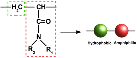
Figure 1: Ad-hoc mapping of the acrylamide family of thermoresponsive polymers. $R_{\rm 1}$ and $R_{\rm 2}$ can be any arbitrary groups. The part of the monomer within the red box may have both hydrophilic and hydrophobic groups due to which it is modeled as an amphiphilic bead.

The amphiphilic bead has attractive interactions with both the solvent and the solvophobic beads. The interaction between the solvophobic bead and the solvent is purely repulsive. The solvent can be introduced either by including it explicitly or by incorporating its effects implicitly within the interaction potentials. Since coarse-grained potentials are obtained by integrating out the internal degrees of freedom of the unit, it is temperature dependent in general. When the scale of coarse graining is small, such a dependence is weak and can be neglected. However, when the solvent is implicit, the interaction potentials have a stronger dependence on the temperature, and the nature of this dependence has to be assumed a priori. To avoid a specifically assumed temperature dependence of the interaction potentials, we explicitly incorporate the solvent. The potential energy for the system is given by the following expression

$$E=\sum_{i=1}^{N-1}k_{\rm b}(b_{i}-b_{i0})^{2}+\sum_{i=1}^{N_{\rm t}}\sum_{j>i}4\epsilon_{ij}\Bigg{[}\left(\frac{\sigma}{r_{ij}}\right)^{12}-\left(\frac{\sigma}{r_{ij}}\right)^{6}-\left(\frac{\sigma}{r_{{\rm c},ij}}\right)^{12}+\left(\frac{\sigma}{r_{{\rm c},ij}}\right)^{6}\Bigg{]},$$ (1)

where $N$ is the number of beads in the polymer chain, as mentioned before. $k_{\rm b}$ the force constant for the bonded interaction, $b_{i}$ the bond length between neighboring beads, $N_{\rm t}$ the total number of beads in the system (polymer + solvent), $b_{i0}$ the equilibrium bond length and $r_{ij}$ the distance between two non-bonded beads. The second term is the Shifted Lennard Jones (SLJ) potential with $r_{{\rm c},ij}$ being the cutoff distance at which the potential is truncated and shifted to zero. The above form of SLJ potential ensures that all the beads are spherically symmetric and have size $\sigma$. All the interaction parameters are kept independent of the temperature. We define dimensionless quantities as $\overline{r}_{ij}=r_{ij}/\sigma$, $\overline{\epsilon}_{ij}=\epsilon_{ij}/\epsilon_{\rm ss}$, $\overline{k}_{\rm b}=\sigma^{2}k_{\rm b}/\epsilon_{\rm ss}$, $\overline{b}_{i0}=b_{i0}/\sigma$, $\overline{T}=k_{\rm B}T/\epsilon_{\rm ss}$, $\overline{P}=\sigma^{3}P/\epsilon_{\rm ss}$ and $\overline{t}=t\sqrt{\epsilon_{\rm ss}/(m\sigma^{2})}$, where $\epsilon_{\rm ss}$ is the potential energy of interaction between two solvent beads. We fix the values to $\overline{b}_{i0}=1$ and $\overline{k}_{\rm b}=200$ for all the simulations. The values of the other interaction parameters are listed in Table 1.

Table 1: Interaction parameters of the SLJ potential. Amphiphilic, solvophobic and solvent are represented by A, H and S, respectively.

$ij$	AA	HH	SS	AH	HS	AS
$\overline{\epsilon}_{ij}\ \ \ \ \$	1	1	1	1	1	1.4, 1.7, 1.8, 2.0
$\overline{r}_{{\rm c},ij}\ \ \ \ \$	2.5	2.5	2.5	2.5	$2^{1/6}$	2.5

Molecular dynamic simulations were performed in an NPT ensemble using the Nose-Hoover thermostat for different temperatures at a constant pressure $\overline{P}=0.002$. The trajectories were generated using the Velocity-Verlet algorithm with a time-step $\Delta\overline{t}=0.004$. The ratio of the number of polymer beads to the solvent beads was maintained at 0.04 for all simulations. Simulations of $N=200$ chain were performed at four different interactions; $\overline{\epsilon}_{\rm AS}=1.4,1.7,1.8,2.0$. For each of these values, the temperature was varied from $\overline{T}=0.5$ to 0.7 with an interval of 0.05. Simulations were also performed for a $N=400$ chain for $\overline{\epsilon}_{\rm AS}=1.7$ at the temperatures ranging from $\overline{T}=0.5$ to 0.8 with an interval of 0.05. The 200 and 400 bead systems were equilibrated for $1\times 10^{8}$ steps, and the data was sampled after every $4\times 10^{6}$ and $2\times 10^{7}$ steps, respectively. Four different initial configurations were used for averaging. All simulations were performed using open source molecular dynamics code LAMMPS.Plimpton1995

The simulation data were used for the calculation of different structural quantities. We calculated the radius of gyration, $R_{\rm g}$, of the polymer to monitor the swelling of the polymer chain. We define a dimensionless radius of gyration $\overline{R}_{\rm g}=R_{\rm g}/\sigma$ given by the following expression

$$\overline{R}_{\rm g}=\sqrt{\frac{1}{N}\sum_{i=1}^{N}(\overline{r}_{i}-\overline{r}_{\rm cm})^{2}},$$ (2)

where $N=200$ and $400$, $\overline{r}_{\rm cm}$ and $\overline{r}_{i}$ are the dimensionless coordinates of the centre of mass of the polymer chain and the $i$-th bead, respectively.

The number of solvent beads, $N_{\rm s}$, in the first solvation shell of the polymer was calculated to determine the bound solvent content. The solvent beads which were within a distance of $\overline{r}=r/\sigma=1.5$ from any of the polymeric beads were regarded to be part of the first solvation shell.

The effective interaction between the polymer beads was calculated using the potential of mean force $U_{\rm AH}$, which was calculated from the radial distribution function of the amphiphilic and solvophobic bead pairs using the following expression:Chandler1987

$$\frac{\overline{U}_{\rm AH}(\overline{r})}{\overline{T}}=-\ln{g_{\rm AH}(\overline{r})}.$$ (3)

where $\overline{U}_{\rm AH}=U_{\rm AH}/\epsilon_{\rm ss}$ is the dimensionless potential of mean force.

II.2 Solvophobic Potential by Kolomeisky and Widom

Our simulations indicate that the LCST is dependent on the entropy loss of the bound solvent, and the mean interaction energy difference between the bulk and the bound solvent (see Sec. III.1). To obtain further insights related to the nature of the transition, scaling behavior, and the effect of chain flexibility, a theoretical approach is adopted where we consider the hydrophobic potential proposed by Kolomeisky and Widom (KW).Kolomeisky1999 The KW model is spherically symmetric in nature and does not relate to a specific solvent or solute, which is in correspondence with the modeling framework employed in our simulations. The KW model belongs to a class of implicit solvent models Lee1996 ; Moelbert2003a which incorporate different interaction energies depending on the proximity of the solvent to a solute molecule. These models have been used for studying the solubility of small solutes in water. The KW model is one of the simplest among these models as it has only two solvent interaction energies; one for the bound state and another for the bulk state. These interaction energies are analogous to the monomer-solvent interaction energy ($\epsilon_{\rm AS}$), and solvent-solvent interaction energy ($\epsilon_{\rm SS}$) in our simulation model, respectively. Hence it can be seen that the model contains those contributions which have been emphasized in our simulation results.

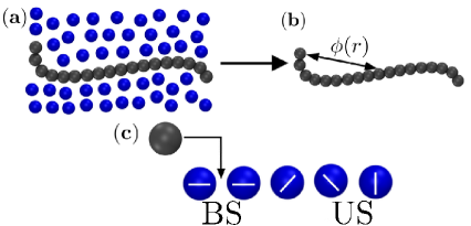
Figure 2: Schematic representation for the theoretical model. Black and blue beads represent monomer and solvent molecules, respectively. (a) Single polymer chain in explicit solvent, (b) single polymer chain in implicit solvent where the effect of solvent is incorporated in the monomer-monomer interaction potential $\phi(r)$, and (c) $\phi(r)$ modeled by the solvophobic potential given by KW.Kolomeisky1999 The potential assumes a one-dimensional solvent lattice where each solvent molecule has $q$ states. Neighboring solvent molecules exist in a bounded state (BS) when both are in the state “1” and in unbounded state (US) state otherwise. Solute can occupy interstitial sites between bounded (BS) solvent molecules.

In the KW-model, solvent molecules form a one-dimensional lattice with a nearest neighbor interaction, and each solvent molecule can exist in $q$ different states denoted by $1,2,\cdots q$ as shown in Fig. 2. The interaction energy between the neighboring solvent molecules is $w$ when both of them are in the state “1”, and $u$ otherwise with $u>w$. Here the former and the latter cases are termed as the bound state (BS) state and the unbound state (US) state, respectively. A solvent molecule in the BS state can exist only in one state, whereas that in the US state in $q-1$ states. Hence the entropy of a solvent molecule in the BS state vanishes, whereas that in the US state is given by $k_{\rm B}\ln{(q-1)}$. In other words, the BS state is energetically favorable ($w<u$), while the US state is entropically favorable. The energetic ($\Delta U$) and entropic ($\Delta S$) differences between the BS and US states are $w-u$ and $-k_{\rm B}\ln{(q-1)}$, respectively. The competition between the BS and the US states can be conveniently described by a dimensionless parameter $x$ defined as

$$x=e^{(\Delta U-T\Delta S)/k_{\rm B}T}=\frac{q-1}{c},$$ (4)

where

$$c=e^{(u-w)/k_{\rm B}T}.$$ (5)

Since the number of states $q$ is constant in the KW model, $x$ is a monotonically increasing function of the temperature. Solute molecules are allowed to occupy only the interstitial sites between the solvent molecules in the BS state. Based on these assumptions, KW obtained the solvent mediated attraction potential $\phi(r)$ between two solute molecules (implicit solvent) for $r>\sigma,$Kolomeisky1999

$$\phi(r)=-k_{\rm B}T\ln{\left[1+\left(\frac{1+Q}{1-Q}\right)\left(\frac{1-S}{1+S}\right)^{(r-\sigma)/\sigma}\right]},$$ (6)

where

$$S=\left[1-\frac{4x}{(1+x)^{2}}\left(1-\frac{1}{c}\right)\right]^{1/2},$$ (7)

$$Q=\frac{\rm\operatorname{sgn}{({\it x}-1)}}{\left[1+4x/(x-1)^{2}c\right]^{1/2}},$$ (8)

and $\operatorname{sgn}(z)$ is the sign function. Fig. 3 shows the variation of $\phi/k_{\rm B}T$ as a function of $\tilde{r}=r/\sigma$ for two different temperatures. The range of the solvent mediated interaction becomes shorter when the temperature is increased. From the inset of Fig. 3, it can be seen that the attraction becomes stronger for higher temperature when $\tilde{r}$ is small. Such a behavior indicates that the monomers tend to aggregate as the temperature is increased.

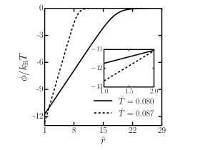
Figure 3: Variation of $\phi/k_{\rm B}T$ as function of $\tilde{r}=r/\sigma$ for different $\tilde{T}$ when $q=5\times 10^{5}$. The inset shows the variation at low $\tilde{r}$ values.

The large value of $q$ used by KW was justified in order to match the temperature dependence of the solubility of non-polar solutes in water.Kolomeisky1999 From Eq. (6) it can be seen that the monomer-monomer potential is temperature dependent due to the implicit nature of solvent. An important point to note is that this temperature dependence is not ad-hoc but a consequence of the underlying solvent model summarized in Fig. 2.

III Results and Discussions

III.1 Simulation

To examine the structural change of the polymer chain with the temperature, we plot in Fig. 4 the variation of $\overline{R}_{\rm g}$ with $\overline{T}$ for different $\overline{\epsilon}_{\rm AS}$ for the $N=200$ chain. The measured $\overline{R}_{\rm g}$ is distinctly larger when $\overline{\epsilon}_{\rm AS}$ is increased, implying swelling as a result of stronger association between the amphiphilic bead and the solvent. We observe that there are three different behaviors according to the value of $\overline{\epsilon}_{\rm AS}$; (i) when $\overline{\epsilon}_{\rm AS}=1.4$, the polymer chain remains in a globular state and its $\overline{R}_{\rm g}$ is almost independent of $\overline{T}$, (ii) when $\overline{\epsilon}_{\rm AS}=2.0$, the polymer chain is in the coiled state at all the temperatures, and (iii) when $\overline{\epsilon}_{\rm AS}=1.7$ and $1.8$, $\overline{R}_{\rm g}$ decreases with the temperature, which is similar to the LCST behavior in thermoresponsive polymers.

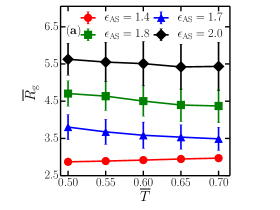
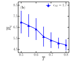
Figure 4: Variation of $\overline{R}_{\rm g}$ of polymer chain with $\overline{T}$ for (a) 200 bead polymer at different values of $\overline{\epsilon}_{\rm AS}$, (b) $N=400$ chain at $\overline{\epsilon}_{\rm AS}=1.7$.

To further probe the decrease in $\overline{R}_{\rm g}$ with the temperature, we focus on the $N=400$ chain for $\overline{\epsilon}_{\rm AS}=1.7$. From Fig. 4, we see that the size change with the temperature for the $N=400$ chain is more prominent compared to that of the $N=200$ chain, which is due to difference in scaling of $\overline{R}_{\rm g}$ with $N$ for the coiled and globular states.Grosberg1997 In Fig. 4, $\overline{R}_{\rm g}$ decreases by 23% as the temperature is increased from $\overline{T}=0.55$ to 0.75. Such trends have been observed in atomistic simulations of PNiPAM-water system.Du2010a ; Alaghemandi2012a ; Deshmukh2012b Unlike the first-order LCST transition behavior observed in experimental studies of thermoresponsive polymer solutions,Wu1998 ; Wang1999 ; Cao2005 the transition observed in Fig. 4 shows a gradual change in $\overline{R}_{\rm g}$ with $\overline{T}$. It is known that the coil-to-globule transition is a first-order transition only in the case of rigid and semirigid chains.Grosberg1992 ; Graziano2000 ; Baysal2003 Hence the continuous transition in our simulation is not surprising because the polymer chain used in the simulations, is fully flexible due to the absence of the angular and dihedral interactions. This is further supported by the results of our theoretical model, where we observe that the coil-to-globule transition deviates from a first order behavior with increase in chain flexibility (see Sec III.2). Based on the above observations, we consider that the behavior observed for $\overline{\epsilon}_{\rm AS}=1.7$ is akin to the LCST phenomenon in thermoresponsive polymers. Figure  5 shows representative snapshots of $N=400$ chain at $\epsilon_{\rm AS}=1.7$ for different temperatures, we can see that the polymer chain is in the coil-like state below $\overline{T}=0.6$, while it is is the globule-like state above $\overline{T}=0.7$.

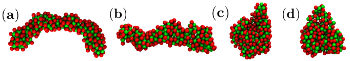
Figure 5: Representative snapshots of equilibrated $N=400$ chain at $\epsilon_{\rm AS}=1.7$ for different temperatures. Green and red beads represent solvophobic and amphiphilic units, respectively. (a) $\tilde{T}=0.55$, (b) $\tilde{T}=0.6$, (c) $\tilde{T}=0.7$ and (d) $\tilde{T}=0.8$. Solvent beads are not included for clarity.

Hereafter we will be referring to $\overline{\epsilon}_{\rm AS}=1.4$, $\overline{\epsilon}_{\rm AS}=1.7$ and $1.8$, and $\overline{\epsilon}_{\rm AS}=2.0$ as low, intermediate and high values, respectively. To further understand the behavior in these three states, we examine the variation of the number of bound solvent beads, $N_{\rm s}$, with the temperature. In Fig. 6, the number of bound solvent is found to be almost independent of $\overline{T}$ for low and high values of $\overline{\epsilon}_{\rm AS}$, whereas it decreases by increasing the temperature for intermediate values. In Fig. 6, we plot $N_{\rm s}$ for the $N=400$ chain as a function of $\overline{T}$, when $\epsilon_{\rm AS}=1.7$. The decrease of $N_{\rm s}$ with the temperature is more prominent as compared with that of the $N=200$ chain case. Moreover, $N_{\rm s}$ markedly decreases around $\overline{T}=0.65$ which coincides with the temperature around which $\overline{R}_{\rm g}$ also decreases (see Fig. 4). It should be stressed that the change in $\overline{R}_{\rm g}$ and $N_{\rm s}$ with the temperature is observed in our model with minimal interactions as in Eq. (1). It is important to note that even when the interaction parameters are independent of the temperature, the temperature dependence of $\overline{R}_{\rm g}$ is induced by the bound solvent number $N_{\rm s}$ for a range of values of $\overline{\epsilon}_{\rm AS}$.

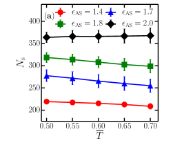
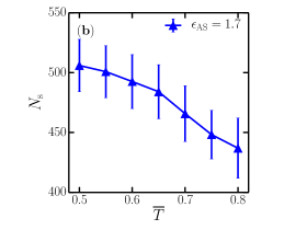
Figure 6: (a) Variation of $N_{\rm s}$ with $\overline{T}$ at different values for (a) $N=200$ chain at different values of $\overline{\epsilon}_{\rm AS}$, (b) $N=400$ chain at $\overline{\epsilon}_{\rm AS}$=1.7.

The above trends in the three different states can be rationalized by considering the different energy, and entropic contributions in the model system. The attraction between the amphiphilic monomer and the solvent is energetically favorable since it is stronger than the solvent-solvent interaction ($\epsilon_{\rm AS}>\epsilon_{\rm SS}$), leading to a coil-like polymer conformation with many bound solvent beads. Whereas from the viewpoint of entropy, the solvent prefers to be in the bulk state rather than the bound state. Another important contribution is the solvation of solvophobic beads, which is unfavorable as the interaction between the solvophobic bead and the solvent is repulsive. The interplay of these contributions determines the different states of the polymer chain.
Concerning intermediate $\overline{\epsilon}_{\rm AS}$ values, the large values of $\overline{R}_{\rm g}$ in the coil-like state (see Fig. 4) and large $N_{\rm s}$ at low temperatures (see Fig. 6) indicate that the attraction between the amphiphilic monomer and the solvent dominates the entropy loss of the solvent. Hence it is favorable for the solvent to solvate the solvophobic beads despite the repulsive interaction between them. With increase in the temperature, the gain in the entropy due to unbinding of the solvent leads to a reduction in the bound solvent content, $N_{\rm s}$. In the transition region ($0.6\leq T\leq 0.7$), there is marked decrease of the bound solvent because the entropy gain of the solvent dominates over the amphiphilic-solvent attraction. This change in the dominant contribution makes the solvation of solvophobic beads unfavorable, leading to an attraction between the polymeric beads. Such an attraction becomes stronger with the temperature, and drives the transition from the coil-like state to the globule-like state. In Fig 7, we plot the potential of mean force, $\overline{U}_{\rm AH}$, between the amphiphilic and the solvophobic beads as a function of the distance $\overline{r}$. Here we see that the attraction between the polymeric beads increases with the temperature. At low temperature, the attraction between the polymeric beads is screened due to the presence of solvent beads. At high temperatures, the bound solvent beads unbind due to entropy gain which reduces the screening effect, leading to the collapse of the polymer. As shown in Fig. 7, the increase in the attraction between polymeric beads with temperature is not observed for low $\overline{\epsilon}_{\rm AS}$ values.
For low $\overline{\epsilon}_{\rm AS}$ values, both $\overline{R}_{\rm g}$ and $N_{\rm s}$ are small. This means that at these interaction strengths the entropic gain of the free solvent beads dominates over the interaction between the amphiphilic monomer and the solvent for all the temperatures. Hence the solvation of solvophobic beads is unfavorable in the entire temperature range. On the other hand, for high $\overline{\epsilon}_{\rm AS}$ values, both $\overline{R}_{\rm g}$ and $N_{\rm s}$ are large. This indicates that the attractive interaction is stronger than the entropy loss which leads to the binding of the solvent to the polymer. Hence, the solvation of the solvophobic beads is favored at all temperatures despite the repulsive interaction between the solvophobic monomer and the solvent.

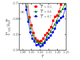
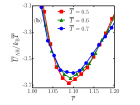
Figure 7: Variation of $\overline{U}_{\rm AH}/k_{\rm B}\overline{T}$ with $\overline{r}$ at different temperatures for (a) $N=400$ chain at $\overline{\epsilon}_{\rm AS}=1.7$ (b) $N=200$ chain at $\overline{\epsilon}_{\rm AS}=1.4$.

We find from our simulations that the transition from the coil-like state to the globule-like state depends on how much the solvophobic beads can be solvated. The solvation depends on the interplay between the entropy loss of the bound solvent, and the energetic difference between the bound and the bulk solvent. The bound solvent is energetically favored as the interaction between the amphiphilic monomer and the solvent is stronger than the solvent-solvent interaction. Therefore two kinds of beads having opposite interactions with the solvent are necessary to exhibit the LCST as long as the interaction parameters are independent of the temperature as in our case. Additionally in our simulation, we did not incorporate any specific chemical or structural details pertaining to the solvent or the polymer chain. Therefore we have demonstrated that the LCST behavior can be exhibited by a coarse-grained description of the polymer and the solvent even when the interaction parameters are independent of the temperature.

III.2 Theoretical description of the coil-to-globule transition

To study the coil-to-globule transition in the theoretical framework, we adopt the phenomenological free energy expression for a polymer chain in an implicit solvent, which has been given by Grosberg and Kuznetsov.Grosberg1992 We choose the KW potential (see Sec II.2) to model the effective monomer-monomer interaction. The free energy expression for the system is as follows:

$$\frac{F}{k_{\rm B}T}=\alpha^{2}+\frac{1}{\alpha^{2}}+\frac{\sqrt{N}}{\alpha^{3}\sigma^{3}}B+\frac{1}{\alpha^{6}\sigma^{6}}C,$$ (9)

where $\alpha=R_{\rm g}/(\sqrt{N}\sigma)$ characterizes the extent of the swelling, $N$ the degree of polymerization, $\sigma$ the diameter of the monomeric unit, $B$ and $C$ are the second and the third virial coefficients, respectively. The first and the second terms in the above free energy are the entropic contributions with the the coiled and the globular states given by $\alpha>1$ and $\alpha<1$, respectively. The third and the fourth terms represent the energy contributions from the two-body and the three-body interactions, respectively. In general, the second virial coefficient $B$ is given by

$$B=2\pi\int_{0}^{\infty}{\rm d}r\,r^{2}\left(1-e^{-\Phi(r)/k_{\rm B}T}\right),$$ (10)

where $\Phi(r)$ is the monomer-monomer interaction potential. Here we assume that it has the following form:

$$\Phi(r)=\left\{\begin{array}[]{ll}\infty&:r<\sigma\\ \phi(r)&:r>\sigma\end{array}\right.,$$ (11)

where $\Phi(r)$ for $r<\sigma$ corresponds to the (hard-core) excluded volume interaction, and $\phi(r)$ for $r>\sigma$ (see Eq. (6)) is the KW solvophobic potential. Substituting Eqs. (6) and  (11) into Eq. (10), we obtain the second virial coefficient $B$ as

$$B=\frac{2\pi\sigma^{3}}{3}\left[1+3\left(\frac{1+Q}{1-Q}\right)\left(\frac{1}{\ln{L}}-\frac{2}{\left(\ln{L}\right)^{2}}+\frac{2}{\left(\ln{L}\right)^{3}}\right)\right],$$ (12)

where $L=(1-S)/(1+S)$.

Hereafter we use the dimensionless quantities such as the temperature $\tilde{T}=k_{\rm B}T/(u-w)$, the distance $\tilde{r}=r/\sigma$, the solvent mediated interaction potential $\tilde{\phi}=\phi/(u-w)$, and the second virial coefficient $\tilde{B}=3B/2\pi\sigma^{3}$. In Fig. 8, we plot $\tilde{B}$ as a function of $\tilde{T}$ for different $q$-values. We observe that $\tilde{B}$ remains almost unity for low temperatures and then decreases rapidly for higher temperatures. This means that the monomer-monomer interaction is repulsive for lower temperatures, while it is attractive for higher temperatures. Moreover, the temperature corresponding to the sharp drop from the positive (repulsive) to the negative (attractive) $\tilde{B}$-values decreases when $q$ is increased for a fixed $u-w$ value. The significance of this observation will be discussed later.

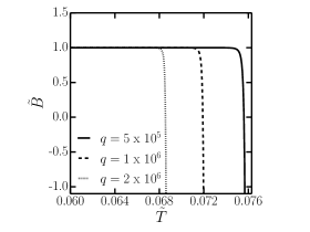
Figure 8: Variation of $\tilde{B}$ with $\tilde{T}$ for different $q$ values.

In order to find the equilibrium polymer conformation, we minimize Eq. (9) with respect to $\alpha$, and obtain the equation

$$\alpha^{5}-\alpha-\pi\sqrt{N}\tilde{B}-\frac{\tilde{C}}{\alpha^{3}}=0,$$ (13)

where $\tilde{C}=3C/\sigma^{6}$ is the non-dimensional third virial coefficient which is related to the rigidity of the polymer chain and has contributions from the three-body interactions such as angular interactions. We numerically solve the above equation to obtain $\alpha$ for fixed values of $q$, $N$ and $\tilde{C}$. In Fig. 9, we show the variation of the swelling parameter $\alpha$ with the temperature $\tilde{T}$ for different values of the third virial coefficient $\tilde{C}$ when $q=5\times 10^{5}$. We see that the polymer chain undergoes a transition from the coiled state to the globular state with increase in the temperature.

For low temperatures, the polymer chain is in the coiled state and hence large $\alpha$. In this case, the first and the third terms in Eq. (13) are dominant because $N$ is also large. Then Eq. (13) reduces to

$$\alpha^{5}-\pi\sqrt{N}\tilde{B}\approx 0,$$ (14)

and we obtain $R_{\rm g}\sim N^{3/5}$ corresponding to the scaling of a polymer chain in a good solvent. When the temperature is high, on the other hand, the polymer is in the globular state and $\alpha$ becomes small. Then the third and the fourth terms dominate in Eq. (13);

$$\pi\sqrt{N}\tilde{B}+\frac{\tilde{C}}{\alpha^{3}}\approx 0.$$ (15)

This gives the scaling $R_{\rm g}\sim N^{1/3}$ corresponding to a polymer chain in a poor solvent.

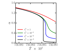
Figure 9: Variation of $\alpha$ with $\tilde{T}$ for different values of $\tilde{C}$ when $q=5\times 10^{5}$ and $N=10^{5}$.

In order to understand this coil-to-globule transition in terms of the dominant interactions, let us consider the free energy difference of a solvent molecule between the BS and US states;

$$\Delta F=F_{\rm BS}-F_{\rm US}=U_{\rm BS}-U_{\rm US}-T(S_{\rm BS}-S_{\rm US}),$$ (16)

where $U_{\rm BS}$ ($U_{\rm US}$) and $S_{\rm BS}$ ($S_{\rm US}$) are the energy and the entropy of the BS (US) state, respectively. Using the model parameters defined in Sec. II.2, the above quantity can be expressed as

$$\Delta F=-(u-w)+k_{\rm B}T\ln{(q-1})=k_{\rm B}T\ln x,$$ (17)

where $x$ is defined before in Eq. (4). From Eq. (17) and since $u>w$, we find $\Delta F<0$ for $x<1$ (lower temperatures), leading to the BS state being more favorable. Given the implicit nature of the solvent in the theoretical treatment, the large value of $\alpha$ for lower temperatures in Fig. 9 is an indication of the large amount of the bound solvent. For $x>1$ (higher temperatures), on the other hand, the US state is more favorable and the amount of the unbound solvent increases. In this case, the attraction between the monomeric units is induced. This is seen in Fig. 8 for the larger negative value of the second virial coefficient $\tilde{B}$. These solvent induced interactions drive the transition from the coiled state to the globular state. The phase transition temperature $T^{\ast}$ determined by the condition $\Delta F=0$ is given by

$$T^{\ast}=\frac{u-w}{k_{\rm B}\ln{(q-1)}}.$$ (18)

As observed in Sec. II.2, $T^{\ast}$ decreases as $q$ is increased when $u-w$ is fixed.

We further observe in Fig. 9 that the nature of the transition changes from a discontinuous transition to a continuous one by increase in the third virial coefficient $\tilde{C}$. It is known that the third virial coefficient is larger for flexible chains.Grosberg1992 ; Graziano2000 This shows that the nature of transition deviates from a first-order behavior with increase in the flexibility of the chain. Another important point is that the above argument does not include any details regrading the structure of the solvent and/or polymer which indicates that the structural details of the bound solvent are not necessary for the thermoresponsive behavior to manifest.

IV Summary and Conclusions

In this paper, we have tried to understand the single chain coil-to-globule transition of a thermoresponsive polymer through simulation and theoretical approaches. In the simulations, the model comprises of a single polymer chain in an explicit solvent with temperature independent interaction parameters. The solvent is explicitly included to avoid any ad-hoc dependence of the interaction potentials on temperature. To obtain further insights, we have adopted a theoretical framework with only those interactions that have been emphasized in our simulation studies. The theoretical model describes a single chain in an implicit solvent where the effect of solvent is included into the monomer-monomer interaction potential. For the interaction between the monomers, we have used the solvophobic potential proposed by Kolomeisky and Widom.Kolomeisky1999 The temperature dependence of the solvophobic potential is not ad-hoc in nature and arises due to the underlying solvent model.
Our simulations indicate that the LCST is dependent on the competition between the two contributions, namely, the entropy loss of the bound solvent and the mean energy difference between the bound and the bulk solvent. This hypothesis is supported by our theoretical calculations. The former favors the globular state of the polymer chain, whereas the latter prefers the coiled state. At low temperatures, solvent molecules bind to the polymer chain rather than to reside in the bulk because the bound state is energetically favorable, and the coiled state is obtained. At high temperatures, on the other hand, the entropy loss of the bound state is more dominant than its energetic gain and the solvent molecules tend to leave the polymer. Such a competition of the interactions induces a solvent driven attraction between the polymeric beads leading to the collapse of the polymer chain. These findings are supported by the experimental studies of Bischofberger and coworkers who showed that the LCST is dependent on the mean energy difference between the bound and bulk solvent.Bischofberger2014 ; Bischofberger2014a
Another common feature between the simulation and the theory is that both of them have spherically symmetric solvent and monomeric beads. This indicates that the structural arrangement of the solvent molecules around the polymer chain is not a necessary component to be considered explicitly for the coil-to-globule transition. In other words, a coarse-grained description of the solvent is sufficient to reproduce the LCST behavior, this observation is in agreement with the experimental results of Bischofberger and coworkers,Bischofberger2014 ; Bischofberger2014a where they show that a coarse-grained representation of the solvent is sufficient to explain the LCST and its variation with different alcohols.
In our simulations studies, it is shown that the LCST is dependent on the amphiphilic-solvent attraction and solvation of the solvophobic beads. This indicates that in the case of temperature-independent interaction parameters, two different kinds of beads with opposite interaction with the solvent are required in the monomeric unit to exhibit LCST. In the theoretical model, the solvent is implicit and the variation of solvent effects with temperature is included in the monomer-monomer interaction due to which one kind of bead is sufficient to exhibit LCST. A mixture of PNiPAM and water exhibits a first-order phase transition at 32$\degree$C.Wang1998 ; Wu1998 In our theoretical argument, we showed that the order of the transition changes from a first-order (discontinuous) to a second-order (continuous) with the increase in the chain flexibility (or the third virial coefficient). The reason why we observe only the continuous coil-to-globule transition in our simulation is because we did not take into account any angular interactions to deal with the chain flexibility. The effect of angular and dihedral interactions on the nature of the coil-to-globule transition needs to be explored further.
The variation in behavior with temperature for different $\overline{\epsilon}_{\rm AS}$ values (see Fig 4) is analogous to different polymers in the family of poly(N,N-alkyl alkyl acrylamide). Low $\overline{\epsilon}_{\rm AS}$ values are similar to polymers with bulky side groups such as poly(N-butyl acrylamide) which are always insoluble in water. On the other hand, high $\overline{\epsilon}_{\rm AS}$ values are similar to polymers such as polyacrylamide which are always soluble in water. This indicates that our coarse-grained model is able to explain the LCST behavior for different systems in the poly(N,N-alkyl,alkyl acrylamide) family of polymers. Furthermore, the model can also be utilized to study the variation of LCST due to factors such as co-solvents and additives by examining their effect on the two dominant physical interactions namely, the entropy loss of the bound solvent and the mean energy difference between the bound and the bulk solvent. This aspect will be addressed in our future studies.

- (1) T. Hoare, J. Santamaria, G. F. Goya, S. Irusta, D. Lin, S. Lau, R. Padera, R. Langer, and D. S. Kohane, Nano Lett. 9, 3651 (2009).
- (2) T. Okano, A. Kikuchi, Y. Sakurai, Y. Takei, and N. Ogata, J. Control. Release. 36, 125 (1995).
- (3) T. R. Hoare and D. S. Kohane, Polymer. 49, 1993 (2008).
- (4) S. Sun, P. Wu, W. Zhang, W. Zhang, and X. Zhu, Soft Matter. 9, 1807 (2013).
- (5) R. O. Costa and R. F. Freitas, Polymer 43, 5879 (2002).
- (6) I. Bischofberger, D. C. E. Calzolari, and V. Trappe, Soft Matter 10, 8288 (2014).
- (7) X. Wang, X. Qiu, and C. Wu, Macromolecules. 31, 2972 (1998).
- (8) C. Wu and X. Wang, Phys. Rev. Lett. 80, 4092 (1998).
- (9) Y. Ono and T. Shikata, J. Am. Chem. Soc. 128, 10030 (2006).
- (10) S. Deshmukh, D. A. Mooney, T. McDermott, S. Kulkarni, and J. M. Don MacElroy, Soft Matter 5, 1514 (2009).
- (11) S. Deshmukh, D. A. Mooney, and J. M. MacElroy, Mol. Simul. 37, 846 (2011).
- (12) M. Alaghemandi and E. Spohr, Macromol. Theory Simulations 21, 106 (2012).
- (13) S. A. Deshmukh, S. K. R. S. Sankaranarayanan, K. Suthar, and D. C. Mancini, J. Phys.Chem. B 116, 2651 (2012).
- (14) A. K. Tucker and M. J. Stevens, Macromolecules 45, 6697 (2012).
- (15) E. Chiessi, A. Lonardi, and G. Paradossi, J. Phys. Chem. B 114, 8301 (2010).
- (16) Y. Zhang, S. Furyk, D. E. Bergbreiter, and P. S. Cremer, J. Am. Chem. Soc. 127, 14505 (2005).
- (17) H. Du, R. Wickramasinghe, and X. Qian, J. Phys. Chem. B 114, 16594 (2010).
- (18) H. G. Schild and D. A. Tirrell, Langmuir 7, 665 (1991).
- (19) V. S. Shinde, M. V. Badiger, A. K. Lele, and R. A. Mashelkar, Langmuir 17, 2585 (2001).
- (20) Y. Mohan, T. Premkumar, D. Joseph, and K. Geckeler, React. Funct. Polym. 67, 844 (2007).
- (21) X. Zhang, Y. Yang, and T. Chung, Langmuir, 18 2538 (2002).
- (22) C. Scherzinger, A. Schwarz, A. Bardow, K. Leonhard, and W. Richtering, Curr. Opin.Colloid Interface Sci. 19, 84 (2014).
- (23) D. Mukherji and K. Kremer, Macromolecules 46, 9158 (2013).
- (24) D. Mukherji, C. M. Marques, and K. Kremer, Nat. Commun. 5, 4882 (2014).
- (25) D. Mukherji, C. M. Marques, T. Stuehn, and K. Kremer, J. Chem. Phys. 142, 114903 (2015).
- (26) J. Walter, V. Ermatchkov, J. Vrabec, and H. Hasse, Fluid Phase Equilib. 296, 164 (2010).
- (27) B. Ray, Y. Okamoto, M. Kamigaito, M. Sawamoto, K.-i. Seno, S. Kanaoka, and S. Aoshima, Polym. J. 37, 234 (2005).
- (28) Y. Katsumoto and N. Kubosaki, Macromolecules 41, 5955 (2008).
- (29) Y. Okada and F. Tanaka, Macromolecules 38, 4465 (2005).
- (30) H. G. Schild, M. Muthukumar and D. A. Tirrell, Macromolecules 24, 948 (1991).
- (31) I. Bischofberger, D. C. E. Calzolari, P. De Los Rios, I. Jelezarov, and V. Trappe, Sci. Rep. 4, 4377 (2014).
- (32) J. A. Anderson and A. Travesset, Macromolecules 39, 5143 (2006).
- (33) S. J. Marrink, H. J. Risselada, S. Yefimov, D. P. Tieleman, and A. H. de Vries, J. Phys.Chem. B 111, 7812 (2007).
- (34) M. Mella and L. Izzo, Polymer 51, 3582 (2010).
- (35) J. M. Polson and N. E. Moore, J. Chem. Phys. 122, 024905 (2005).
- (36) M. Hatakeyama and R. Faller, Phys. Chem. Chem. Phys. 9, 4662 (2007).
- (37) A. B. Kolomeisky and B. Widom, Faraday Discuss. 112, 81 (1999).
- (38) S. Plimpton, J. Comput. Phys. 117, 1 (1995).
- (39) D. Chandler, Introduction to modern statistical mechanics (Oxford University Press, New York, Oxford, 1987).
- (40) B. Lee and G. Graziano, J. Am. Chem. Soc. 118, 5163 (1996).
- (41) S. Moelbert and P. D. L. Rios, Macromolecules 36, 5845 (2003).
- (42) A. Y. Grosberg and A. R. Khokhlov, Giant molecules: here, and there, and everywhere (Academic Press, New York, USA, 1997).
- (43) S. A. Deshmukh, S. K. R. S. Sankaranarayanan, K. Suthar, and D. C. Mancini, J. Phys.Chem. B 116, 2651 (2012).
- (44) X. Wang and C. Wu, Macromolecules 32, 4299 (1999).
- (45) Z. Cao, W. Liu, P. Gao, K. Yao, H. Li, and G. Wang, Polymer 46, 5268 (2005).
- (46) A. Y. Grosberg and D. V. Kuznetsov, Macromolecules 25, 1970 (1992).
- (47) G. Graziano, Int. J. Biol. Macromol. 27, 89 (2000).
- (48) B. M. Baysal and F. E. Karasz, Macromol. Theory Simul 12, 627 (2003).