The use of the multi-cumulant tensor analysis for the algorithmic optimisation of investment portfolios.

Abstract

The cumulant analysis plays an important role in non Gaussian distributed data analysis. The shares’ prices returns are good example of such data. The purpose of this research is to develop the cumulant based algorithm and use it to determine eigenvectors that represent investment portfolios with low variability. Such algorithm is based on the Alternating Least Square method and involves the simultaneous minimisation $2$’nd – $6$’th cumulants of the multidimensional random variable (percentage shares’ returns of many companies). Then the algorithm was tested during the recent crash on the Warsaw Stock Exchange. To determine incoming crash and provide enter and exit signal for the investment strategy the Hurst exponent was calculated using the local DFA. It was shown that introduced algorithm is on average better that benchmark and other portfolio determination methods, but only within examination window determined by low values of the Hurst exponent. Remark that the algorithm of is based on cumulant tensors up to the $6$’th order calculated for a multidimensional random variable, what is the novel idea. It can be expected that the algorithm would be useful in the financial data analysis on the world wide scale as well as in the analysis of other types of non Gaussian distributed data.

Keywords

cumulant tensors, ALS–class algorithm, Hurst exponent, financial data analysis, stock exchange.

1 Introduction

Let us consider the multidimensional frequency distribution of shares’ prices’ percentage returns. The optimization (minimization) of higher cumulants of this distribution is used to determine investment portfolios, to test if they are better on average than the benchmark, during the crash. The proposed procedure is based on [1] and implies the investigation of cumulants tensors – the $n$’th cumulant of the multidimensional random variable is represented by the $n$–dimensional tensor [1, 2]. For this purpose, I introduce the generalisation of the classical Value at Risk (VaR) procedure [3], where the left Eigenvector Decomposition (EVD) of the second cumulant (the covariance) matrix is performed, and the multidimensional normal distribution of financial data is assumed. In classical EVD approach, the portfolio with minimal variance corresponds to the last eigenvector. However, the classical EVD method fails to anticipate the risk of investment portfolios since the second cumulant fails to represent the extreme events, where drops of shares’ prices values are high and cross–correlated. This happens mainly due to the break down of the central limit theorem resulting from the time–varying variance of financial data. The Autoregressive Conditional Heteroskedasticity (ARCH), that violates both independence and identical distribution assumptions of the central limit theorem, was recorded for many types of financial data [4, 5, 6, 7, 8]. Recall also the impact of long range auto–correlations of shares’ returns [9, 10, 11, 12, 13, 14]. It is worth to mention the work [15, 16], where authors shows that moments or cumulants (of order $6$ or $8$) may be necessary to account for the severe price fluctuations, that are usually observed at short time scales (e.g. portfolio rebalanced at a weekly, time scales). In my research I would examine portfolio rebalanced at the $20$ trading days (approximately monthly scale) as it is often performed in practice in assets management. To search for the severe price fluctuations I used the Hurst exponent indicator.

Following this arguments, high cumulants analysis should anticipate extreme events, improving the search for portfolios with low variability. There are some works implying the use of $2$’nd, $3$’rd and $4$’th cumulant of multivariate shares’ returns [17, 18]. In this research I use the $5$’th and the $6$’th cumulant as well, what is a new approach for multivariate shares’ returns. In general the proposed algorithm is based on the High Order Singular Value Decomposition (HOSVD) and Alternating Least Square (ALS) procedure [2]. To compare the proposed method with others (such as EVD), the author, for each method, creates the family of investment portfolios which are supposed to be safer than a benchmark. Then portfolios are compared using the result function that is an average percentage change of portfolios’ values – an average portfolio results. Other result functions are also discussed:

1. a mode of percentage change of portfolios’ values,

2. a maximal loss / minimal gain – the result of the “worst portfolio”,

3. a minimal loss/ maximal gain – the result of the “best portfolio”.

The major motivation for this research is to introduce the automation method of analysis of data that are not Gaussian distributed. Good example of such data are financial data, especially during the rupture and crash period. It is why, I focus in this work, on the financial data analysis. To determine the rupture and crash period and introduce the enter and exit signal of an investment strategy, I use the Hurst exponent indicator calculated for the WIG20 index, using the local DFA. This paper give some additional incentive for the development of cumulants tensors calculation method at low computational complexity. Afterwards the multi–cumulant analysis may be applied for large financial data sets and tested against many crashes on many markets. Additionally the method may be used to analyse other (non–financial) data that are not Gaussian distributed.

2 The classical approach, the covariance matrix EVD

Let us take the $M$–dimensional random variable of size $T$, $\textbf{X}\in\mathbb{R}^{(T\times M)}$, being the percentage returns of $M$ shares. Its marginal variables are $X_{i}$, and values are $x_{t,i}$:

$$\textbf{X}=[X_{1},\ldots,X_{i},\ldots,X_{M}]=\left[\begin{array}[]{ccc}x_{t=1,1}&\cdots&x_{t=1,M}\\ \vdots&\vdots&\vdots\\ x_{t=T,1}&\cdots&x_{t=T,M}\\ \end{array}\right].$$ (1)

An unbiased estimator of variance of the $i$’th marginal random variable ($X_{i}$) is:

$$\sigma^{2}_{i}=\frac{1}{T-1}\sum_{t=1}^{T}(x_{t,i}-\overline{X_{i}})^{2},$$ (2)

and an unbiased estimator of covariance between ($X_{i}$) and ($X_{j}$) is:

$$\textrm{cov}_{i,j}=\frac{1}{T-1}\sum_{t=1}^{T}(x_{t,i}-\overline{X_{i}})(x_{t,j}-\overline{X_{j}}).$$ (3)

The variance and the covariance can be represented by the $M\times M$ symmetric covariance matrix, called also the second cumulant matrix – $C_{2}$ (notice $\sigma_{i}^{2}=\textrm{cov}_{i,i}$):

$$C_{2}=\left[\begin{array}[]{cccc}\sigma^{2}_{1}&\textrm{cov}_{1,2}&\cdots&\textrm{cov}_{1,L}\\ \textrm{cov}_{2,1}&\sigma^{2}_{2}&\cdots&\textrm{cov}_{2,L}\\ \vdots&\vdots&\ddots&\vdots\\ \textrm{cov}_{L,1}&\textrm{cov}_{L,2}&\cdots&\sigma^{2}_{L}\\ \end{array}\right].$$ (4)

Definition 2.1.

The Eigenvalue Decomposition – EVD. Consider the covariance (second cumulant) symmetric matrix. The matrix can be diagonalized in the following way:

$$C_{2}=V\Sigma V^{\intercal},$$ (5)

where $\Sigma=V^{\intercal}C_{2}V$ is the diagonal matrix with diagonal values $\sigma^{\prime 2}_{i}=(V^{\intercal}C_{2}V)_{ii}$ and $V$ is unitary $M\times M$ factors matrix, such that $\sigma^{\prime 2}_{i}$ are sorted in descending order:

$$\Sigma=\left[\begin{array}[]{cccc}\sigma^{\prime 2}_{1}&0&\cdots&0\\ 0&\sigma^{\prime 2}_{2}&\cdots&0\\ \vdots&\vdots&\ddots&\vdots\\ 0&0&\cdots&\sigma^{\prime 2}_{M}\\ \end{array}\right].$$ (6)

The $i$’th column of $V$ is the eigenvector that corresponds with the eigenvalue $\sigma^{\prime 2}_{i}$. Rows in the $i$’th column of $V$ are factors that give the linear combination of marginal random variables with the combination’s variance $\sigma^{\prime 2}_{i}$. The last eigenvector would give the linear combination of marginal random variables with the smallest combination’s variance – $\sigma^{\prime 2}_{M}$.

The classical EVD procedure has been often used in the portfolio risk determination. However, it requires the multidimensional Gaussian distribution of shares’ returns, where all information about the variability of the frequency distribution is stored in the covariance matrix. As mentioned before the financial data (shares’ returns) are not Gaussian distributed and the classical EVD procedure has often failed in the investment portfolio’s risk determination [19]. It is why the author proposes to extend the classical EVD procedure by taking into consideration also cumulants of order higher than $2$ – the higher cumulants.

3 Cumulants

Let us consider the $M$ dimensional random variable $\textbf{X}=[X_{1},\ldots,X_{M}]$. The $n$’th cumulant $C_{n}$ of such variable is the $n$–mode tensor [2], with elements $\kappa_{\alpha_{1},\ldots,\alpha_{n}}(\textbf{X})$ [20, 21]:

$$\kappa_{\alpha_{1},\ldots,\alpha_{n}}(\textbf{X})=\frac{\partial^{n}}{\partial\tau_{\alpha_{1}},\partial\tau_{\alpha_{2}},\ldots,\partial\tau_{\alpha_{n}}}\log\left(E\left(\exp(\tau\cdot\textbf{X}^{\intercal})\right)\right)\bigg{|}_{\tau=0}.$$ (7)

where $\tau$ is the argument vector $\tau=\underbrace{[\tau_{1},\cdots,\tau_{i},\cdots\tau_{M}]}_{M}$, and $E()$ is the expected value operator. Formulas used to calculate cumulants up to $4$’th order are well known [20, 21]. The author has calculated $5$’th and $6$’th cumulants by the direct use of (7). Here analysed data were substituted for the random variable $\textbf{X}\in\mathbb{R}^{(T\times M)}$, and computer differentiations were performed at point $\tau=\underbrace{[\tau_{1},\cdots\tau_{M}]}_{M}=0$, using ForwardDiff and DualNumbers library in Julia programming [22].

3.1 The multi–cumulant decomposition.

To investigate the financial data the author takes many cumulant tensors $C_{2},\dots,C_{n}$, where $n=4$ or $n=6$. The calculation of cumulants of order $n>6$ might require larger data series, but non–stationary of financial data [10] makes the investigation of long time series less adequate than shorter data series. To achieve the factor matrix $V$, the author proposes the following ALS–class algorithm, where the search for the local maximum of the function $\Phi(V)$ is performed [23, 24]. Following the maximisation procedure which can not be solved precisely, the author will find the local maximum using the iteration procedure [24] and show that the results are meaningful.

Definition 3.1.

The $\Phi(V)$ function. Consider the $i$’th core–tensor $T_{i}$ that is the contraction of $C_{i}$ tensor and $i$ factor matrices $V$:

$$(T_{i})_{l_{1},\cdots,l_{i}}=\sum_{j_{1},\cdots,j_{i}}(C_{i})_{j_{1},\cdots,j_{i}}V_{j_{1}l_{1}}\cdots V_{j_{i}l_{i}}.$$ (8)

The ALS procedure proposed in [1, 24] refers to the search for the common factor matrix $V$ that maximise $\Phi_{4}(V)$.

$$\Phi_{4}(V)=\frac{1}{2!}||V^{\intercal}C_{2}V||^{2}+\sum_{i=3}^{4}\frac{1}{i!}||T_{i}||^{2}.$$ (9)

The author proposes to extend the analysis up to the $6$’th cumulant which are more sensitive to extreme “tail events”. Hence the author defines $\Phi_{6}(V)$:

$$\Phi_{6}(V)=\frac{1}{2!}||V^{\intercal}C_{2}V||^{2}+\sum_{i=3}^{6}\frac{1}{i!}||T_{i}||^{2}.$$ (10)

To find the common factor matrix $V$, the ALS–based algorithm is proposed by author and presented at subsection (3.2). The idea of the algorithm is based on the algorithm proposed in [23] where the iteration procedure was used for the search for the local maximum of the following function:

$$\Phi^{\prime}(V)=||V^{\intercal}C_{2}V||^{2}+\alpha_{n}||T_{n}||^{2}.$$ (11)

The proposed algorithm works for the general case (any $\Phi_{n}(V)$), but computations were performed for $n=4$ and $n=6$. Racall that ALS algorithms move information into the upper left corner of the core–tensor and order the information in the sense of the Frobenius Norm. Take the linear transformation of analysed data X:

$$\textbf{Y}=\textbf{X}V,$$ (12)

where $\textbf{Y}=[Y_{1},\ldots,Y_{j},\dots,Y_{M}]$. Here $Y_{j}$ represents percentage returns of the $j$’th portfolio. Elements of Y are:

$$y_{t,j}=\sum_{i=1}^{M}x_{t,i}V_{i,j}$$ (13)

The rear columns of the factor matrix would give the investment portfolio with little variability.

3.2 The algorithm.

The algorithm used to determine the factor matrix $V$ given cumulant symmetric tensors $C_{2}\cdots C_{n}$, it is a general algorithm and work for each $n\geq 3$. Let ${C_{i}}_{(1)}$ be the unfold of the tensor $C_{i}$ in the first mode [2]. The first factor matrix anzatz is computed as a matrix that columns are left eigenvectors of the following matrix:

$$\left[\frac{C_{2}}{2!}\cdots\frac{{C_{i}}_{(1)}}{i!}\cdots\frac{{C_{n}}_{(1)}}{n!}\right]$$ (14)

At $k$’th interaction, we have the $(V_{k-1})$ factor matrix. Now the following procedure is performed. The contraction of the $C_{i}$ tensor (matrix) and $i-1$ factor matrices $(V_{k-1})$ is performed:

$$(S_{i})_{j_{1},l_{2}\cdots,l_{i}}=\sum_{j_{2},\cdots,j_{i}}(C_{i})_{j_{1},j_{2}\cdots,j_{i}}(V_{k-1})_{j_{2}l_{2}}\cdots(V_{k-1})_{j_{i}l_{i}}.$$ (15)

To compute $V_{k}$ we takes left eigenvectors of the following matrix:

$$\left[\frac{S_{2}}{2!}\cdots\frac{{S_{i}}_{(1)}}{i!}\cdots\frac{{S_{n}}_{(1)}}{n!}\right]$$ (16)

The procedure is repeated to satisfaction the stop condition.

4 The investigation of financial data.

The cumulant analysis was performed in the optimal portfolios searching problem. Let us consider the price of a $i$’th share at time $t$ – $p_{t,i}$. Its percentage return is

$$x_{t,i}=\frac{p_{t,i}-p_{(t-1),i}}{p_{(t-1),i}}\cdot 100\%.$$ (17)

In our case $t$ numerates trading days (the analyse of daily returns was performed) and $p_{t,i}$ the closing price of $i$’th share the given trading day numbered by $t$. Next the multidimensional random variable X of percentage returns is constructed. To construct investment portfolios we use the factor matrix $V$. The $j$’th portfolio returns are one dimensional random variable $Y_{j}$ with elements $y_{t,j}$.

The naive method of factor matrix determination uses the Eigenvalue Decomposition (EVD) of the covariance matrix [3]. This procedure is not fully adequate since shares returns are not Gaussian distributed, especially the rupture and crisis period [9, 10, 11, 12] – importantly such period can be predicted by the use of the Hurst exponent. To anticipate higher cumulants of shares returns as well, the author proposes to determine the factor matrix $V$ by searching for the local maximum of the $\Phi_{4}(V)$ function as well as $\Phi_{6}(V)$ function – using cumulant tensors up to the $6$’th order, what is a new approach. The proposed $\Phi_{6}(V)$ method is used to chose portfolios with returns that have low absolute values of high cumulants. Hence the method is supposed to work well where the portfolio’s variability is a disadvantage. It happens during the crash of the financial market, hence the author tests the method during the last rupture and crisis on the Warsaw Stock Exchange.

4.1 The data analysis.

The author has examined $M=10$ dimensional random variable Tab. (1), being daily percentage returns of the shares of $10$ most liquid companies from the WIG20 index at the time 12.05.2010 – 04.08.2016 (the WIG20 index includes $20$ most liquid companies traded on the Warsaw Stock Exchange). Recent composition of the WIG20 index is presented in Fig. (1)

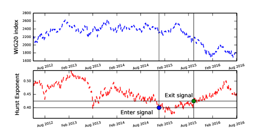
Figure 1: WIG20 index and the Hurst exponent.

The WIG20 index reached maximum at 14.05.2015 and then has fallen rapidly – the crash has occurred. To introduce the signal of incoming crash, the Hurst exponent was calculated for the WIG20 index using the local Detrended Fluctuation Analysis (DFA) [10, 13].

$i$	company	contribution	contribution to
		to WIG20 %	benchmark % $(BP_{i})$
1	PKOBP	14.64	18.31
2	PZU	14.04	17.55
3	PEKAO	11.65	14.57
4	PKNORLEN	8.45	10.57
5	PGE	7.52	9.40
6	KGHM	7.14	8.93
7	BZWBK	5.21	6.51
8	LPP	4.77	5.96
9	PGNIG	3.55	4.43
10	MBANK	3.00	3.75

Table 1: the 10 most liquid companies of the WIG20 index, their value contribution to the WIG20 index (at 20.03.2015) and as their value contribution to proposed benchmark portfolio.

4.1.1 The Hurst exponent.

To determine the rupture and crisis period of the stock exchange, where the examined investment strategy was tested the Hurst exponent was calculated using the local DFA. The parameters for DFA were the same as in [25]: $500$ days long observation window was used to examine past closing value of the WIG20 index. Having the Hurst exponent, I introduce the signals of entry and exit for proposed investment strategy. Recall that in [10] the Hurst exponent was calculated using the local DFA for the index of Polish Stock Exchange, and it was shown that before a crash (near a rupture point), the Hurst Exponent has minima $\lesssim 0.4$. Hence the entry threshold value was chosen as $H_{entry}=0.4$. The exit threshold was chosen as $H_{exit}=0.425$ – data with high negative auto–correlation was chosen for a test.

Regarding the recent crash the entry signal occurred at 19.12.2014 and the exit signal at 10.09.2015. To examine the algorithm, I introduce the $20$ trading days (approx. 1 months) long investment windows – as it is performed in practice assets management. First window starts a day after the enter signal – 22.12.2014, and there are $9$ windows within a test period 22.12.2014 – 27.01.2015, 27.01.2015 – 24.02.2015, 24.02.2015 – 24.03.2015, 24.03.2015 – 23.04.2015, 23.04.2015 – 22.05.2015, 22.05.2015 – 22.06.2015, 22.06.2015 – 20.07.2015, 20.07.2015 – 17.08.2015, 17.08.2015 – 14.09.2015 (the last window ends just after exit point). For each window, cumulants are calculated using a test series of length $T=1100$, that ends just before the examination window. Next investment returns are analysed for data in given window – the testing set. In next subsections the analysis is discussed in details for the $7$’th window of 22.06.2015 – 20.07.2015. Then the analysis results are presented for other windows.

4.1.2 Optimal portfolios determination – training.

Let us discuss in details the procedure for the exemplary window of 22.06.2015 – 20.07.2015. Given the training set, the factor matrix is determined using different methods, such as EVD, $\Phi_{4}(V)$ and $\Phi_{6}(V)$. Here also the Independent Component Analysis (ICA) was used for more general comparison. The $\Phi_{4}(V)$ method requires the calculation of $3$’rd and $4$’th cumulants. For $\Phi_{6}(V)$ also $5$’th and $6$’th cumulant tensors are required, which were calculated by the direct use of Eq. (7). Given $\Phi_{4}(V)$ and $\Phi_{6}(V)$ the algorithm introduced in subsection (3.2) was used for the factor matrix $V$ determination.

In Fig. (2) some cumulant value of the one dimensional random variable, that is the $j$’th investment portfolio $Y_{j}$ (with elements $y_{t,i}=\sum_{i=1}^{M}x_{t,i}V_{i,j}$) are presented for different methods of the factor matrix determination. Generally large cumulants values were stored in first portfolios where $j=1,2,\cdots$. For further investigation I took the $5$ rear portfolios, where $j\in[5,10]$ as those that have low cumulants’ absolute values.

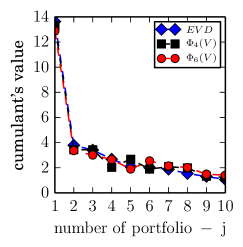
(a) second cumulant

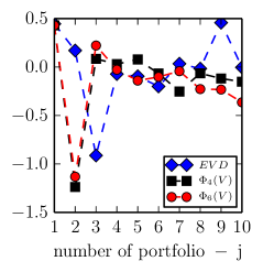
(b) third cumulant (normalized)

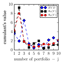
(c) fourth cumulant (normalized)

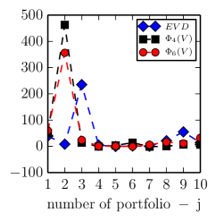
(d) sixth cumulant (normalized)

Figure 2: Values of cumulants for portfolios, the larger $j$ the portfolio is supposed to be less “variable”.

4.1.3 Testing optimal portfolios.

After the training (the determination of $V$) has been completed, the testing of portfolios is performed. The factor matrices ($V$) columns contain both positive and negative values, the later corresponds to the negative value of shares in the portfolio – the short sale. To diminish the use of the sort sale, the test portfolios were compared with the benchmark portfolio. Shares values contributions in benchmark portfolio – $BP_{i}$ are given in Tab. (1). In proposed test portfolios the value contribution of the $i$’th share in the $j$’th portfolio would be:

$${}TV_{i,j}=\frac{\alpha BP_{i}+V_{i,j}}{\sum_{i=1}^{10}\left(\alpha BP_{i}+V_{i,j}\right)},$$ (18)

the $\alpha=7$ was taken, to make cases of the short sale rare. For testing, shares prices of companies, see Tab. (1) were taken. Testing set is represented by: ${p_{t^{\prime},i}}$, where $t^{\prime}$ is time in the testing window. The percentage return of $j$’th portfolio after $L$ trading days is:

$$Pr_{j}(L)=\frac{\sum_{i=1}^{10}TV_{i,j}\left(\frac{p_{(t^{\prime}=L+1,i)}}{p_{(t^{\prime}=1,i)}}\right)-\sum_{i=1}^{10}TV_{i,j}}{\sum_{i=1}^{10}TV_{i,j}}=\sum_{i=1}^{10}TV_{i,j}\left(\frac{p_{(t^{\prime}=L+1,i)}}{p_{(t^{\prime}=1,i)}}\right).$$ (19)

In Fig. (3), returns after $10$ and $20$ trading days are presented. Remark, in this research transaction costs were not taken into account. The benchmark portfolio contributions can be reproduced by simply substituting $\forall_{i,j}\ V_{i,j}=0$ to Eq. (18).

4.2 Discussion.

Analysing Fig. (3), one can see that the $\Phi_{6}(V)$ method gives in both cases $3$ portfolios that are better than the benchmark and $2$ that are as good as benchmark. In the reminding part of the paper, I discuss the statistics of returns of such $5$ portfolios.

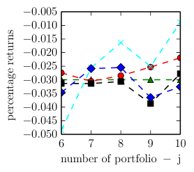
(a) After $10$ trading days

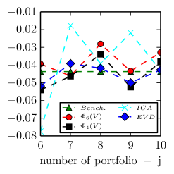
(b) After $20$ trading days

Figure 3: Returns of $5$ portfolios, investments window 22.06.2015 – 20.07.2015.

One can also conclude, that each method of factor matrix determination ($\Phi_{6}(V)$, $\Phi_{4}(V)$, EVD, ICA) produces the worst portfolio

$$\min_{j\in[6,10]}Pr_{j}(L),$$ (20)

which return is minimal and often smaller than benchmark’s return. Those minimum of portfolios’ returns are presented in Fig. (4a). Analysing minimum of portfolios’ returns one can conclude that out of all methods ($\Phi_{6}(V)$, $\Phi_{4}(V)$, EVD, ICA) the $\Phi_{6}(V)$ method gives smallest loss – its worst portfolio is almost as good as benchmark. The worst results gives the ICA method, this is due to large variability of returns – see Fig. (3), such method is not desirable during a crisis. Similarly best portfolios can found:

$$\max_{j\in[6,10]}Pr_{j}(L),$$ (21)

Their results are presented in Fig. (4b). Best results presents the ICA, however this method is not safe. Next best are $\Phi_{6}(V)$ and $\Phi_{4}(V)$.

It is worth checking now, which portfolio determination method is best on average. In Fig.  (4c), mean values of portfolios’ returns are presented:

$$\frac{1}{5}\sum_{j=6}^{10}Pr_{j}(L).$$ (22)

Remark that all methods but $\Phi_{6}(V)$ give an average return similar to or worse than the benchmark. It is a worthy result, since it is hard to beat the benchmark on average.

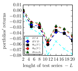
(a) minimum of portfolio’s returns

(b) maximum of portfolio’s returns

(c) mean of portfolio’s returns

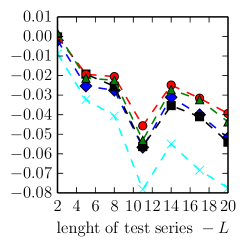
(d) mode of portfolio’s returns

Figure 4: Statistics of investment returns, $7$’th window of 22.06.2015 – 20.07.2015.

To examine a typical portfolio, the mode of portfolios’ returns can be mentioned as well – see Fig. (4d), here $\Phi_{6}(V)$ gives results, better than other methods, and slightly better the the benchmark. Concluding, statistics of the $\phi_{6}(V)$ method are better than other methods and the benchmark. Results of other $20$ days observation windows within the observation period determined by the Hurst exponent and outside it are discussed in next subsection.

4.3 All observation windows.

The analysis was performed for following observation windows: 22.12.2014 – 27.01.2015, 27.01.2015 – 24.02.2015, 24.02.2015 – 24.03.2015, 24.03.2015 – 23.04.2015, 23.04.2015 – 22.05.2015, 22.05.2015 – 22.06.2015, 22.06.2015 – 20.07.2015, 20.07.2015 – 17.08.2015, 17.08.2015 – 14.09.2015. The first window starts a trading day after the enter signal recorded at 19.12.2014. The WIG20 index increased in first for windows, the maximum appeared in the $5$’th window where the crisis started, the last ($9$’th window) ends just after the exit signal recorded at 10.09.2015. Windows $5$ – $9$ are crisis windows. Since I an interested in the investment strategy outcome between the enter and the exit signal, I present the cumulative results of investment that starts a trading day after the enter signal and ends just after exit signal. For each window factor matrices are calculated separately, investment is made at the first point in a window, at the last point of the window shares are sold and the mean of returns of $5$ portfolios is calculated. Cumulative of such mean returns are presented in Fig. (5a). In Fig. (5b) the cumulative results are presented for crisis portfolios $5$ - $9$, here investment starts at 23.04.2015.

(a) whole investment 22.12.2014 – 14.09.2015

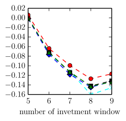
(b) crisis windows 23.04.2015 – 14.09.2015

Figure 5: Cumulative of means of portfolios returns.

In Fig. (6) similar results are presented, but now mode of returns of $5$ portfolios is calculated in each window and the cumulative results are presented. Analysing Fig. (5, 6) one can conclude that the $\Phi_{6}(V)$ method on average gives best results at the exit point and during the crisis.

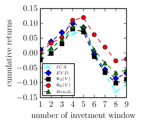
(a) whole investment 22.12.2014 – 14.09.2015

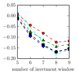
(b) crisis windows 23.04.2015 – 14.09.2015

Figure 6: Cumulative of modes of portfolios returns.

In Fig. (7a) cumulative results are presented, if in each window the worst portfolio was chosen (unlucky choice) – there $\Phi_{6}(V)$ method is worse than a benchmark, but slightly better than other methods. In Fig. (7b) cumulative results are presented, if in each window the best portfolio was chosen (lucky choice) – there $\Phi_{6}(V)$ method is better than all other methods apart from ICA. However the ICA produces also very bad portfolios (worst minimum), and hence is not adequate for a crisis.

(a) Cumulatives of minima of returns

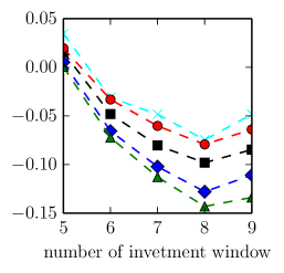
(b) Cumulatives of maxima of returns

Figure 7: Best and worst cumulative result at crisis windows 23.04.2015 – 14.09.2015.

To test a method a bit more, I introduced observation windows after the exit signal, and number them as $10$’th to $15$’th, the cumulative results of means and modes of portfolio returns are presented in (8). Investment starts at 14.09.2015 and investment windows are 14.09.2015 – 12.10.2015, 12.10.2015 – 09.11.2015, 09.11.2015 – 08.12.2015, 08.12.2015 – 12.01.2016 and 12.01.2016 – 09.02.2016. It can be concluded that beyond the exit signal the $\Phi_{6}(V)$ method gives results similar to other methods and the benchmark. Hence the use of the Hurst exponent to determine the proper enter and exit signal appears to be crucial.

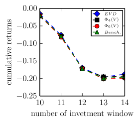
(a) Cumulatives of means of returns

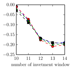
(b) Cumulatives of modes of returns

Figure 8: Statistics for investment after exit signal, 14.09.2015 – 09.02.2016

5 Conclusions

The author has used the multi–cumulant tensor analysis to analyse financial data and determine optimal investment portfolio with low absolute values of cumulants of their percentage returns. For this purpose, the author has analysed daily returns of shares traded on the Warsaw Stock Exchange to determine the factor matrix that represents such portfolios and test them during the recent rupture and crash period on the Warsaw Stock Exchange.

The main result of this work is the introduction of the algorithm that uses $2$’nd – $6$’th cumulant tensors to analyse multivariate financial data and determine the investment portfolios that have low variability (low cumulants’ absolute values). The Hurst exponent, calculated by the local DFA for the WIG20 index, indicates the auto–correlation phase on the stock market (the rupture period and the early stage of the crisis). At this phase, the introduced method is on average better than the benchmark and other tested methods. Importantly the Hurst exponent condition appears to be necessary to achieve this result. The examination of the method can be extended in further research, e.g. the algorithm can be tested on many stock exchanges. The algorithm can also be used to analyse other (non–financial) data that are non–Gaussian distributed.

References

- [1] J. Morton, “Algebraic models for multilinear dependence,” 2009.
- [2] T. G. Kolda and B. W. Bader, “Tensor decompositions and applications,” SIAM review, vol. 51, no. 3, pp. 455–500, 2009.
- [3] P. Best, Implementing value at risk. John Wiley & Sons, 2000.
- [4] V. Akgiray, “Conditional heteroscedasticity in time series of stock returns: Evidence and forecasts,” Journal of business, pp. 55–80, 1989.
- [5] T. Bollerslev, “A conditionally heteroskedastic time series model for speculative prices and rates of return,” The review of economics and statistics, pp. 542–547, 1987.
- [6] T. Bollerslev, R. Y. Chou, and K. F. Kroner, “Arch modeling in finance: A review of the theory and empirical evidence,” Journal of econometrics, vol. 52, no. 1-2, pp. 5–59, 1992.
- [7] R. F. Engle and K. F. Kroner, “Multivariate simultaneous generalized arch,” Econometric theory, vol. 11, no. 01, pp. 122–150, 1995.
- [8] G. W. Schwert and P. J. Seguin, “Heteroskedasticity in stock returns,” the Journal of Finance, vol. 45, no. 4, pp. 1129–1155, 1990.
- [9] B. B. Mandelbrot, The variation of certain speculative prices. Springer, 1997.
- [10] D. Grech and G. Pamuła, “The local hurst exponent of the financial time series in the vicinity of crashes on the polish stock exchange market,” Physica A: Statistical Mechanics and its Applications, vol. 387, no. 16, pp. 4299–4308, 2008.
- [11] Ł. Czarnecki, D. Grech, and G. Pamuła, “Comparison study of global and local approaches describing critical phenomena on the polish stock exchange market,” Physica A: Statistical Mechanics and its Applications, vol. 387, no. 27, pp. 6801–6811, 2008.
- [12] G. L. Vasconcelos, “A guided walk down wall street: an introduction to econophysics,” Brazilian Journal of Physics, vol. 34, no. 3B, pp. 1039–1065, 2004.
- [13] K. Domino, “The use of the hurst exponent to predict changes in trends on the warsaw stock exchange,” Physica A: Statistical Mechanics and its Applications, vol. 390, no. 1, pp. 98–109, 2011.
- [14] K. Domino, “The use of the hurst exponent to investigate the global maximum of the warsaw stock exchange wig20 index,” Physica A: Statistical Mechanics and its Applications, vol. 391, no. 1, pp. 156–169, 2012.
- [15] Y. Malevergne and D. Sornette, “Multi-moments method for portfolio management: Generalized capital asset pricing model in homogeneous and heterogeneous markets,” Available at SSRN 319544, 2002.
- [16] M. Rubinstein, E. Jurczenko, and B. Maillet, Multi-moment asset allocation and pricing models, vol. 399. John Wiley & Sons, 2006.
- [17] J. C. Arismendi and H. Kimura, “Monte carlo approximate tensor moment simulations,” Available at SSRN 2491639, 2014.
- [18] E. Jondeau, E. Jurczenko, and M. Rockinger, “Moment component analysis: An illustration with international stock markets,” Swiss Finance Institute Research Paper, no. 10-43, 2015.
- [19] U. Cherubini, E. Luciano, and W. Vecchiato, Copula methods in finance. John Wiley & Sons, 2004.
- [20] M. G. Kendall et al., “The advanced theory of statistics.,” The advanced theory of statistics., no. 2nd Ed, 1946.
- [21] E. Lukacs, “Characteristics functions,” Griffin, London, 1970.
- [22] J. Revels, T. Papamarkou, and M. Lubin, “Forwarddiff.jl,” JuliaDiff/ForwardDiff.jl, 2015.
- [23] L. De Lathauwer and J. Vandewalle, “Dimensionality reduction in higher-order signal processing and rank-(r 1, r 2,…, r n) reduction in multilinear algebra,” Linear Algebra and its Applications, vol. 391, pp. 31–55, 2004.
- [24] B. Savas and L.-H. Lim, “Quasi-newton methods on grassmannians and multilinear approximations of tensors,” SIAM Journal on Scientific Computing, vol. 32, no. 6, pp. 3352–3393, 2010.
- [25] K. Domino and T. Błachowicz, “The use of copula functions for modeling the risk of investment in shares traded on the warsaw stock exchange,” Physica A: Statistical Mechanics and its Applications, vol. 413, pp. 77–85, 2014.