Signatures and conditions for phase band crossings in periodically driven integrable systems

Abstract

We present generic conditions for phase band crossings for a class of periodically driven integrable systems represented by free fermionic models subjected to arbitrary periodic drive protocols characterized by a frequency $\omega_{D}$. These models provide a representation for the Ising and $XY$ models in $d=1$, the Kitaev model in $d=2$, several kinds of superconductors, and Dirac fermions in graphene and atop topological insulator surfaces. Our results demonstrate that the presence of a critical point/region in the system Hamiltonian (which is traversed at a finite rate during the dynamics) may change the conditions for phase band crossings that occur at the critical modes. We also show that for $d>1$, phase band crossings leave their imprint on the equal-time off-diagonal fermionic correlation functions of these models; the Fourier transforms of such correlation functions, $F_{\vec{k}_{0}}(\omega_{0})$, have maxima and minima at specific frequencies which can be directly related to $\omega_{D}$ and the time at which the phase bands cross at ${\vec{k}}={\vec{k}}_{0}$. We discuss the significance of our results in the contexts of generic Hamiltonians with $N>2$ phase bands and the underlying symmetry of the driven Hamiltonian.

I Introduction

Non-equilibrium dynamics of closed quantum systems has been a subject of intense theoretical and experimental research in recent years pol1 ; dziar1 ; dutta1 ; marcos1 . Such systems are known to show several interesting features which have no analogs in their equilibrium counterparts. Some such phenomena include Kibble-Zurek scaling of defect density upon passage through a quantum critical point kz1 ; pol2 ; ks1 ; pol3 ; sondhi0 or a critical (gapless) region ds1 . In addition, such drives may lead to dynamic transitions which cannot be characterized by any local order parameter mukh1 ; pol4 ; dytr1 ; dytr2 ; dutta2 but manifest themselves in the vanishing of the Loschmidt overlap $F(t)=\langle\psi_{i}|\exp[-iH_{f}t]|\psi_{i}\rangle$, where $|\psi_{i}\rangle$ is the initial system wave function (often chosen to be the ground state of $H_{i}$) and $H_{f}$ is the final Hamiltonian following a quench of a Hamiltonian parameter. Such dynamical phase transitions can be defined in terms of non-analyticities (also known as Fischer zeroes) of the dynamical free energy of the system $f(z)=-\lim_{L\to\infty}\ln(F(z))/L^{d}$, where $z$ is obtained by analytic continuation of time $t$ in the complex plane. Finally, quantum quenches may lead to novel properties of the work distribution of quantum systems following the quench which are qualitatively different from their equilibrium counterparts silva1 ; silva2 .

Out of the drive protocols studied theoretically and experimentally so far, periodic drives are found to lead to a gamut of interesting phenomena which do not have counterparts in aperiodically driven systems. These include dynamics induced freezing where the state of the system, after several or single cycle(s) of the drive, has close to unity overlap with its initial state; such a phenomenon can be related to Stuckelberg interference between quantum states of the driven system arnab1 ; pekker1 ; uma1 . In addition, we may use periodic drives to obtain novel steady states in many-body localized systems where a fast drive may lead to delocalization while a slow drive keeps the system localized arnab2 . Moreover, it was shown that periodically driven interacting systems may lead to stable out-of-equilibrium phases in the presence of disorder roderich1 ; such phases are, similar to their equilibrium counterparts, amenable to symmetry based classification sondhi1 . Furthermore, the work distribution of periodically driven system shows an oscillatory behavior with the drive frequency; such a behavior constitutes an example of a quantum interference effect shaping the behavior of a thermodynamic quantity in a closed quantum system arnab3 . Finally, periodically driven integrable systems are known to undergo a separate class of dynamical phase transitions; these transitions, in contrast to the ones discussed for aperiodically driven systems, leave their mark through a change in the convergence of local correlation functions to their steady state values; they can be shown to be a consequence of a change in topology of the Floquet spectrum of the driven system as a function of the drive frequency asen1 .

Apart from the effects mentioned earlier, another widely studied phenomenon that occurs in periodically driven clean quantum systems involves the generation of topological phases characterized by non-trivial edge modes even when the starting ground state of the corresponding equilibrium Hamiltonian is topologically trivial kita1 ; lind1 ; jiang ; gu ; kita2 ; lind2 ; morell ; trif ; russo ; basti1 ; liu ; tong ; cayssol ; rudner ; basti2 ; tomka ; gomez ; dora ; katan ; kundu ; basti3 ; schmidt ; reynoso ; wu ; perez ; thakurathi1 ; reichl ; thakurathi2 . Such systems have been treated both analytically and numerically demonstrating the appearance of edge modes after a drive through one or more time periods signifying that the system has entered a topological phase. Recently, however, a more complete understanding of generation of edge states due to periodic drives in clean systems has been put forth in Ref. rudner1, in terms of the properties of the time evolution operator $U(t,0)\equiv U(t)$ given by

$$U(t) = {\mathcal{T}}_{t}e^{-(i/\hbar)\int_{0}^{t}dt^{\prime}H(t^{\prime})},\quad 0\leq t\leq T,$$ (1)

where $H(t)$ denotes the periodically driven Hamiltonian of the system, ${\mathcal{T}}_{t}$ denotes time-ordering, we have chosen the initial time $t_{i}=0$ without loss of generality, and here and in the rest of the work we shall denote $T=2\pi/\omega_{D}$ to be the drive period, where $\omega_{D}$ is the drive frequency. It was pointed out in Refs. rudner1, and rudner2, that the knowledge of $U(T)=\exp[-iH_{F}T/\hbar]$, or equivalently the Floquet Hamiltonian $H_{F}$, is insufficient for describing the topological properties of the system. Such properties can be understood instead by tracking the crossings of the phase bands $\phi_{n}({\vec{k}},t)$ which are defined using the expression of $U_{{\vec{k}}}(t)$ for $t\leq T$ as

$$U_{{\vec{k}}}(t)=\sum_{n=1}^{n_{\rm max}}P_{n}({\vec{k}};t)e^{i\phi_{n}({\vec{k}};t)}.$$ (2)

Here we have assumed that the crystal momentum ${\vec{k}}$ is a good quantum number, $n$ is the band index with $n_{\rm max}$ bands for each ${{\vec{k}}}$, $\lambda_{n}(\vec{k},t)=\exp[i\phi_{n}({\vec{k}},t)]$ are eigenvalues of $U_{\vec{k}}(t)$, and $P_{n}({\vec{k}}t)$ projects $U_{{\vec{k}}}(t)$ to its $n^{\rm th}$ eigenstate. We note that $U_{{\vec{k}}}(0)=1$ indicates that $\phi_{n}({\vec{k}},0)=2\pi m$, where $m\in Z$. Thus the phase bands may be represented either in the repeated zone scheme or the reduced zone scheme where the $(n_{\rm max}+1)^{\rm th}$ band is identified with the $n=1$ band. In what follows, we shall adopt the latter representation.

It was shown in Ref. rudner1, that the topological properties of such periodic driven systems may be understood in terms of phase band crossings. As argued in Ref. rudner1, , phase band crossings are topologically significant only if they occur between the first and the top bands of the reduced Brillouin zone; all other crossings can be gauged away by simple deformations of the drive protocol. Each such topologically non-trivial crossing is associated with a finite topological charge $q_{i}$; the number of edge modes which result from such a crossing can be directly related to $q_{i}$. For example in $d=2$, where each phase band can be represented by a Chern number $C_{n}$, the number of chiral edge states within the $m^{\rm th}$ bulk Floquet band is given by $n_{\rm edge}(m)=\sum_{n=1,M}C_{n}-\sum_{i}q_{i}$. Further, it was shown in several earlier works jiang ; rudner1 ; carp1 that the presence of particle-hole and time-reversal symmetries may lead to further restrictions on such crossings; for example, in the presence of particle-hole symmetry and for one-dimensional (1D) driven Hamiltonians, the phase band crossings can occur only at $k_{0}=0$ or $\pi/a$, where $a$ is the lattice spacing of the model (which we will subsequently set equal to $1$, unless mentioned otherwise). The number of edge modes in these systems are completely determined by the parity of the number of such crossings at $k_{0}=0$ and $\pi$ rudner1 ; comment1 . However, the earlier works on phase band crossing did not systematically study the role of the drive protocol; further the conditions for such crossings has not been methodically investigated in terms of the parameters of the driven Hamiltonian beyond a few simple protocols and toy models kita1 ; lind1 ; jiang ; zhao . In this work, we aim to fill up this gap.

To this end, we study a class of periodically driven integrable models whose Hamiltonian can be represented by free fermions in $d$-dimensions:

$$H(t)=\sum_{{\vec{k}}}\psi_{{\vec{k}}}^{\dagger}H_{{\vec{k}}}(t)\psi_{\vec{k}},$$ (3)

where $\psi_{{\vec{k}}}=(c_{{\vec{k}}},c_{-{\vec{k}}}^{\dagger})^{T}$ is the two-component fermionic field, $c_{{\vec{k}}}$ are the annihilation operators for the fermions, and $H_{k}(t)$ is given by

$$H_{{\vec{k}}}=(g(t)-b_{{\vec{k}}})\tau^{z}+(\Delta_{{\vec{k}}}\tau^{+}+\rm{H.c.}),$$ (4)

where $g(t)$ is a periodic function of time characterized by a frequency $\omega_{D}$, and $\Delta_{{\vec{k}}}$ can be an arbitrary function of momenta. We note that this kind of Hamiltonian represents a wide class of spin and fermionic integrable models such as the Ising and $XY$ models in $d=1$ subir1 , the Kitaev model in $d=2$ kit1 ; nussinov1 , triplet and singlet superconductors in $d>1$, and Dirac fermions in graphene and atop topological insulator surfaces graphene1 ; topo1 . In what follows, we shall obtain our results by analyzing fermionic systems given by Eq. (4) and point out the relevance of these results in the context of specific models in appropriate places.

The main results that we obtain from such an analysis are the following. First, we obtain an expression for the phase bands corresponding to Hamiltonians given by Eq. (4) within the adiabatic-impulse approximation nori1 ; kanu1 ; child1 for arbitrary drive protocols. Using these expressions and other general arguments, we chart out the most general conditions that need to be satisfied for these phase bands to cross. The conditions that we obtain conform to those obtained earlier for particle-hole symmetric Hamiltonians rudner1 and for specific drive protocols thakurathi1 ; thakurathi2 ; however it constitutes a more general result which holds for arbitrary periodic drive protocols and irrespective of the symmetry of the underlying Hamiltonian. Second, we show that traversing a critical point during such periodic dynamics may lead to qualitatively different band crossing conditions, and we discuss its implications for the properties of the driven system. Third, for $d>1$, we compute the off-diagonal fermionic correlation function $F_{{\vec{k}}}(t)=\langle c_{\vec{k}}^{\dagger}c_{-{\vec{k}}}^{\dagger}\rangle$ and show that the Fourier transform of this correlator will exhibit maxima and minima at specific frequencies $\omega_{0}$ for $\vec{k}=\vec{k}_{0}$ at which the bands cross; we provide an explicit relation between $\omega_{0}$, $\omega_{D}$ and the band crossing time $t_{0}$ for several drive protocols. Thus we show that $F_{\vec{k}_{0}}(\omega_{0})$ carries information about the phase band crossing time $t_{0}$. Finally, we comment on the applicability of our results to general Hamiltonians with $N>2$ phase bands and present a discussion of the role of symmetries of the underlying Hamiltonian in the phase band crossings.

The plan of the rest of the paper is as follows. In Sec. II, we derive explicit expressions for the phase bands within adiabatic-impulse approximation, obtain the conditions for their crossings, and point out the role of critical points for such crossings. This is followed by Sec. III, where we chart out the behavior of $F_{{\vec{k}}_{0}}(\omega_{0})$ and discuss the signatures of phase band crossings which can be inferred from its behavior. Finally, we discuss the significance of our results for more general phase band models, point out the role of symmetries for such crossings, and conclude in Sec. IV.

II Phase band crossings

In this section, we first obtain an expression for the phase bands corresponding to the Hamiltonian in Eq. (4) within the adiabatic-impulse approximation for an arbitrary continuous time protocol in Sec. II.1. This will be followed by an analysis of the obtained expression for $U_{{\vec{k}}}(t)$ leading to the phase band crossing conditions in Sec. II.2.

II.1 Expression for the phase bands

To obtain an expression for $U_{{\vec{k}}}(t)$ for an arbitrary drive protocol $g(t)$, which is characterized by a frequency $\omega_{D}$, we use an adiabatic-impulse approximation which has been used extensively for two-level systems nori1 ; kanu1 ; child1 . We envisage a drive protocol which starts at $t_{i}=0$ and continues till the end of one drive period $t_{f}=T$. In the rest of this section, we shall mostly work in the adiabatic basis in which the wave function at any time $t$ is given by

$$|\psi_{{\vec{k}}}\rangle(t) = c_{1{\vec{k}}}(t)\left(\begin{array}[]{c}u_{0{\vec{k}}}(t)\\ v_{0{\vec{k}}}(t)\end{array}\right)+c_{2{\vec{k}}}(t)\left(\begin{array}[]{c}-v_{0{\vec{k}}}(t)\\ u_{0{\vec{k}}}(t)\end{array}\right),$$ (9)

where $|\psi_{{\vec{k}}}^{g}(t)\rangle=(u_{0{\vec{k}}}(t),v_{0{\vec{k}}}(t))^{T}$ and $-E_{{\vec{k}}}(t)$ are the instantaneous ground state wave function and energy which are given by

$$u_{0{\vec{k}}}(t) = -\frac{\Delta_{{\vec{k}}}}{D_{{\vec{k}}}(t)},\quad v_{\vec{k}}(t)=\frac{E_{{\vec{k}}}(t)+g(t)-b_{{\vec{k}}}}{D_{{\vec{k}}}(t)},$$

$$E_{{\vec{k}}}(t) = \sqrt{(g(t)-b_{{\vec{k}}})^{2}+|\Delta_{{\vec{k}}}|^{2}},$$ (10)

$$D_{{\vec{k}}}(t) = \sqrt{(E_{{\vec{k}}}(t)+g(t)-b_{{\vec{k}}})^{2}+|\Delta_{{\vec{k}}}|^{2}}.$$

The corresponding excited state wave function and energies are given by $|\psi_{{\vec{k}}}^{e}(t)\rangle=(-v_{0{\vec{k}}}(t),u_{0\vec{k}}(t))^{T}$ and $E_{{\vec{k}}}(t)$. We note here that the adiabatic and the diabatic bases are connected by the standard transformation

$$\left(\begin{array}[]{c}|\psi_{{\vec{k}}}^{g}(t)\rangle\\ |\psi_{{\vec{k}}}^{e}(t)\rangle\end{array}\right) = \left(\begin{array}[]{cc}\mu_{{\vec{k}}}(t)&\sqrt{1-\mu_{{\vec{k}}}^{2}(t)}\\ -\sqrt{1-\mu^{2}_{{\vec{k}}}(t)}&\mu_{{\vec{k}}}(t)\end{array}\right)\left(\begin{array}[]{c}|\psi_{{\vec{k}}}^{g}\rangle\\ |\psi_{{\vec{k}}}^{e}\rangle\end{array}\right)$$ (17)

$$\mu_{{\vec{k}}}(t) = u_{0{\vec{k}}}(t)u_{0{\vec{k}}}+v_{0{\vec{k}}}(t)v_{0{\vec{k}}},$$ (18)

where $u_{0{\vec{k}}}\equiv u_{0{\vec{k}}}(t=0)$, similar notations have been used for all other quantities, and in the rest of this section we shall assume the system to be in its initial ground state at $t=0$. The unitary evolution operator $U_{{\vec{k}}}(t)$ relates, by definition, the wave function at time $t$ to the initial wave function and thus satisfies

$$|\psi_{{\vec{k}}}(t)\rangle = U_{{\vec{k}}}(t)|\psi_{{\vec{k}}}^{g}\rangle.$$ (19)

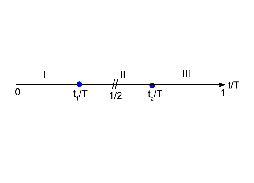
Figure 1: Schematic representation of the time-evolution of a periodically driven system for a drive cycle $T=2\pi/\omega_{D}$. The system reaches the critical points at $t=t_{1{\vec{k}}}\equiv t_{1}$ and $t_{2{\vec{k}}}\equiv t_{2}$. The half-period $t=T/2$ is marked with a hash. The adiabatic regimes before and after the first crossing of critical point are marked as regions I and II respectively, while that after the second crossing of the critical point is marked as region III. See text for details.

The time evolution of a system described by Eq. (4) is sketched in Fig. 1. We divide the time evolution into three distinct regions as shown in Fig. 1. Within the adiabatic-impulse approximation, regions I, II and III are adiabatic regions. In these regions, the system is sufficiently far way from the critical points, crossed at times $t_{1{\vec{k}}}$ and $t_{2\vec{k}}$, so that the instantaneous energy gap for any ${\vec{k}}$ satisfies the Landau criterion: $2E_{{\vec{k}}}^{2}(t)\gg dE_{{\vec{k}}}(t)/dt$. It can be shown that in this regime the system merely gathers kinetic phase nori1

$$U^{\prime}_{{\vec{k}}}(t_{f},t_{i}) = \exp[-i\xi_{{\vec{k}}}(t_{f},t_{i})\tau^{z}],$$

$$\xi_{{\vec{k}}}(t_{f},t_{i}) = \int_{t_{i}}^{t_{f}}dtE_{{\vec{k}}}(t)$$

$$\left(\begin{array}[]{c}c_{1{\vec{k}}}(t_{f})\\ c_{2{\vec{k}}}(t_{f})\end{array}\right) = U^{\prime}_{{\vec{k}}}(t_{f},t_{i})\left(\begin{array}[]{c}c_{1{\vec{k}}}(t_{i})\\ c_{2{\vec{k}}}(t_{i})\end{array}\right).$$ (24)

In the impulse region, the adiabaticity condition given by the Landau criteria breaks down. For slow enough drives, this happens around the critical point and for momentum modes sufficiently close to the critical mode. The key idea of the adiabatic-impulse approximation is to approximate the impulse region to be an infinitesimally small region around the critical point; such an approximation holds good for large amplitude and low frequency drives nori1 ; kanu1 ; child1 . The impulse region is typically reached twice during a drive cycle for any momenta ${\vec{k}}$, at $t=t_{1{\vec{k}}}$ and $t_{2{\vec{k}}}=2\pi/\omega_{D}-t_{1{\vec{k}}}$, where $g(t_{1(2){\vec{k}}})=b_{{\vec{k}}}$. Around $t=t_{1(2){\vec{k}}}$, we can linearize the diagonal terms of the Hamiltonian (Eq. (4)) and obtain

$$H_{{\vec{k}}}^{\rm imp} = v_{{\vec{k}}}(t-t_{1(2){\vec{k}}})\tau^{z}+(\Delta_{{\vec{k}}}\tau^{+}+{\rm H.c.}),$$ (25)

where $v_{{\vec{k}}}=\partial g(t_{1(2){\vec{k}}})/\partial t$. comment2 The probability of excitation between the ground and excited states at each ${\vec{k}}$ can be read off from Eq. (25) as nori1

$$p_{{\vec{k}}} = \exp[-2\pi\delta_{{\vec{k}}}],\quad\delta_{{\vec{k}}}=|\Delta_{{\vec{k}}}|^{2}/|2v_{{\vec{k}}}|.$$ (26)

We note that $p_{{\vec{k}}}=1$ for an unavoided level crossing which happens for the critical mode (where $\Delta_{{\vec{k}}}=0$ and $g(t)-b_{{\vec{k}}}$ crosses zero), while it is zero if $\Delta_{{\vec{k}}}=0$ but $g(t)\neq b_{{\vec{k}}}$ at any point of time during the drive. It was shown in Ref. kanu1, that within this approximations we can define a transfer matrix

$$S_{{\vec{k}}} = \left(\begin{array}[]{cc}\sqrt{1-p_{{\vec{k}}}}e^{-i\tilde{\phi}_{s{\vec{k}}}}&-\sqrt{p_{{\vec{k}}}}\\ \sqrt{p_{{\vec{k}}}}&\sqrt{1-p_{{\vec{k}}}}e^{i\tilde{\phi}_{s{\vec{k}}}}\end{array}\right),$$ (29)

$$\phi_{s{\vec{k}}} = \frac{\pi}{4}+\delta_{{\vec{k}}}\left(\ln\delta_{{\vec{k}}}-1\right)+{\rm Arg}~{}\Gamma(1-i\delta_{{\vec{k}}}),$$ (30)

where $\phi_{s{\vec{k}}}$ is the Stoke’s phase and $\tilde{\phi}_{s\vec{k}}=\phi_{s\vec{k}}-\pi$. The change of wave functions across the first transition point can be obtained using the transfer matrix $S_{{\vec{k}}}$ as

$$\left(\begin{array}[]{c}c_{1{\vec{k}}}(t_{1{\vec{k}}}+\epsilon)\\ c_{2{\vec{k}}}(t_{1{\vec{k}}}+\epsilon)\end{array}\right) = S_{{\vec{k}}}\left(\begin{array}[]{c}c_{1{\vec{k}}}(t_{1{\vec{k}}}-\epsilon)\\ c_{2{\vec{k}}}(t_{1{\vec{k}}}-\epsilon)\end{array}\right),$$ (35)

where $\epsilon>0$ is infinitesimally small. An analogous condition with $S$ replaced by $S^{T}$ (where the superscript $T$ denotes transpose) holds for the second transition point.

Having obtained these relations, we now obtain explicit analytical expressions for the evolution operator $U_{{\vec{k}}}(t)$ in each of the three regions shown in Fig. 1. In region I, the system starts from the ground state so that $c_{1{\vec{k}}}(0)=1$ and $c_{2{\vec{k}}}=0$, Before crossing the critical point for the first time, the dynamics is purely adiabatic leading to (using Eqs.  (9) and (24))

$$c_{1{\vec{k}}}^{I}(t) = \exp[-i\xi_{{\vec{k}}}(t,0)],\quad c_{2{\vec{k}}}^{I}(t)=0.$$ (36)

Using Eqs. (9), (18) and (36), we thus obtain

$$|\psi_{{\vec{k}}}(t)\rangle = e^{-i\xi_{{\vec{k}}}(t,0)}\left(\mu_{{\vec{k}}}(t)|\psi_{{\vec{k}}}^{g}\rangle+\sqrt{1-\mu_{{\vec{k}}}(t)^{2}}|\psi^{e}_{{\vec{k}}}\rangle\right).$$

Using Eqs. (19) and (II.1) and the fact that $U_{{\vec{k}}}(t)$ is a unitary matrix, we obtain for region I

$$U_{{\vec{k}}}^{I}(t) = \left(\begin{array}[]{cc}\mu_{{\vec{k}}}(t)e^{-i\xi_{{\vec{k}}}(t,0)}&-\sqrt{1-\mu_{{\vec{k}}}^{2}(t)}e^{i\xi_{{\vec{k}}}(t,0)}\\ \sqrt{1-\mu_{{\vec{k}}}^{2}(t)}e^{-i\xi_{{\vec{k}}}(t,0)}&\mu_{{\vec{k}}}(t)e^{i\xi_{{\vec{k}}}(t,0)}\end{array}\right).$$ (40)

The eigenvalues $\lambda_{\pm{\vec{k}}}^{I}(t)$ of $U_{{\vec{k}}}^{I}(t)$ provide an expression for the phase bands in region I and are given by

$$\lambda_{\pm{\vec{k}}}^{I}(t) = e^{\pm i\phi_{{\vec{k}}}^{I}(t)},$$

$$\cos[\phi_{{\vec{k}}}^{I}(t)] = \mu_{{\vec{k}}}(t)\cos(\xi_{{\vec{k}}}(t,0)).$$ (42)

An exactly similar method can be used to compute the evolution operators in regions II and III. For example, in region II, using Eqs. (9), (24), (29), and (30), we obtain

$$\left(\begin{array}[]{c}c_{1{\vec{k}}}^{II}(t)\\ c_{2{\vec{k}}}^{II}(t)\end{array}\right) = U^{\prime}_{{\vec{k}}}(t,t_{1\vec{k}})S_{{\vec{k}}}U^{\prime}_{{\vec{k}}}(t_{1{\vec{k}}},0)\left(\begin{array}[]{c}1\\ 0\end{array}\right),$$ (47)

which leads to

$$c_{1{\vec{k}}}^{II}(t) = \sqrt{1-p_{{\vec{k}}}}e^{-i\zeta_{1{\vec{k}}}^{II}(t)},\quad c_{2{\vec{k}}}^{II}(t)=\sqrt{p_{{\vec{k}}}}e^{i\zeta_{2{\vec{k}}}^{II}(t)},$$

$$\zeta_{1{\vec{k}}}^{II}(t) = \tilde{\phi}_{s{\vec{k}}}+\xi_{{\vec{k}}}(t,0),$$

$$\zeta_{2{\vec{k}}}^{II}(t) = \xi_{{\vec{k}}}(t_{1{\vec{k}}},0)-\xi_{{\vec{k}}}(t,t_{1{\vec{k}}}).$$ (48)

Using Eqs. (18), (19) and (48), we then obtain

$$(U^{II}_{{\vec{k}}}(t))_{11} = c_{1{\vec{k}}}^{II}(t)\mu_{{\vec{k}}}(t)+c_{2{\vec{k}}}^{II}(t)\sqrt{1-\mu_{{\vec{k}}}^{2}(t)},$$

$$(U^{II}_{{\vec{k}}}(t))_{21} = c_{2{\vec{k}}}^{II}(t)\mu_{{\vec{k}}}(t)-c_{1{\vec{k}}}^{II}(t)\sqrt{(1-\mu_{{\vec{k}}}^{2}(t)},$$ (49)

$$(U^{II}_{{\vec{k}}}(t))_{22}^{\ast} = (U^{II}_{{\vec{k}}}(t))_{11},\quad(U^{II}_{{\vec{k}}}(t))_{12}^{\ast}=-(U^{II}_{{\vec{k}}}(t))_{21}.$$

The expression for the phase bands in region II may be obtained by diagonalizing the evolution matrix $U_{{\vec{k}}}^{II}(t)$. A straightforward calculation yields the expressions for the eigenvalues of $U_{{\vec{k}}}^{II}(t)$ as $\lambda_{\pm\vec{k}}^{II}(t)=\exp[\pm i\phi_{{\vec{k}}}^{II}(t)]$, where

$$\cos[\phi_{{\vec{k}}}^{II}(t)] = \mu_{{\vec{k}}}(t)\sqrt{1-p_{{\vec{k}}}}\cos(\zeta_{1{\vec{k}}}^{II}(t))$$ (50)

$$+\sqrt{p_{{\vec{k}}}(1-\mu_{{\vec{k}}}^{2}(t))}\cos(\zeta^{II}_{2{\vec{k}}}(t)).$$

A similar calculation can be carried out in region III. Here one finds that

$$\left(\begin{array}[]{c}c_{1{\vec{k}}}^{III}(t)\\ c_{2{\vec{k}}}^{III}(t)\end{array}\right) = U^{\prime}_{{\vec{k}}}(t,t_{2\vec{k}})S^{T}_{{\vec{k}}}U^{\prime}_{{\vec{k}}}(t_{2{\vec{k}}},0)\left(\begin{array}[]{c}1\\ 0\end{array}\right),$$ (55)

where $S_{{\vec{k}}}^{T}$ is the transpose of $S_{{\vec{k}}}$ (Eqs. (29) and (30)). A straightforward calculation then leads to

$$c_{1{\vec{k}}}^{III}(t) = (1-p_{{\vec{k}}})e^{-i\zeta_{1\vec{k}}^{III}(t)}+p_{{\vec{k}}}e^{-i\zeta_{2{\vec{k}}}^{III}(t)},$$

$$c_{2{\vec{k}}}^{III}(t) = \sqrt{p_{{\vec{k}}}(1-p_{{\vec{k}}})}e^{i\phi_{s{\vec{k}}}}\left(e^{-i\zeta_{1{\vec{k}}}^{III}(t)}-e^{-i\zeta_{2{\vec{k}}}^{III}(t)}\right),$$

$$\zeta_{1{\vec{k}}}^{III}(t) = 2\tilde{\phi}_{s{\vec{k}}}+\xi_{{\vec{k}}}(t,0),$$

$$\zeta_{2{\vec{k}}}^{III}(t) = \xi_{{\vec{k}}}(t_{1{\vec{k}}},0)-\xi_{{\vec{k}}}(t_{2{\vec{k}}},t_{1{\vec{k}}})+\xi_{{\vec{k}}}(t,t_{2{\vec{k}}}).$$ (56)

Using Eqs. (18), (19) and (48), we obtain $U_{{\vec{k}}}^{III}(t)$ in an analogous manner. The expressions for the phase bands in region III are then obtained by diagonalizing $U_{{\vec{k}}}^{III}$ and yield $\lambda_{\pm\vec{k}}^{III}(t)=\exp[\pm i\phi_{{\vec{k}}}^{III}(t)]$, where

$$\cos[\phi_{{\vec{k}}}^{III}(t)]=\mu_{{\vec{k}}}(t)\left((1-p_{{\vec{k}}})\cos(\zeta_{1{\vec{k}}}^{III}(t))\right.$$

$$+\left.p_{{\vec{k}}}\cos(\zeta_{2{\vec{k}}}^{III}(t))\right)+\sqrt{p_{{\vec{k}}}(1-p_{{\vec{k}}})(1-\mu_{{\vec{k}}}^{2}(t))}$$

$$\times\left(\cos(\zeta^{III}_{1{\vec{k}}}(t)-\tilde{\phi}_{s{\vec{k}}})-\cos(\zeta^{III}_{2{\vec{k}}}(t)-\tilde{\phi}_{s{\vec{k}}})\right).$$ (57)

Eqs. (42), (50), and (57) constitute the central results of this section. These equations provide us with analytic expressions for the phase bands for integrable models studied for an arbitrary continuous time protocol. In what follows, we shall analyze these expressions to obtain conditions for phase band crossings for these models.

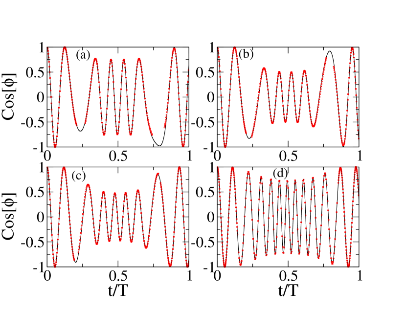
Figure 2: A plot of $\cos(\phi_{k}(t))$ as a function of $t/T$ for (a) $k=\pi/20$, (b) $k=\pi/10$, (c) $k=\pi/6$, and (d) $k=\pi/3$ for the 1D Ising model in a transverse field for the drive protocol $h(t)=h_{0}+h_{1}\cos(\omega_{D}t)$ with $h_{0}=1.1$, $h_{1}=-1$, and $\omega_{D}=0.1$ with all energy scales measured in units of $J$, and $\hbar$ is set equal to unity. The black solid line correspond to exact numerical solution of Eqs. (58), while the red dotted lines correspond to those obtained using adiabatic-impulse approximation (Eqs. (42), (50), and (57)). The match between the two deteriorates with increasing $\omega_{D}$ except at $k=0,\pi$ where the approximation yields exact results.

Before ending this section, we provide a comparison between the exact numerical values of the phase bands with those obtained by our method for the $d=1$ Ising model in a transverse field. As is well-known, Eq. (4) provides a fermionic representation of the transverse field Ising model with $b_{k}=\cos k$, $\Delta_{k}=\sin k$ and $g(t)=h(t)$, where we have set the nearest-neighbor coupling $J$ between the spins and the lattice spacing $a$ to unity subir1 . The critical point for this system is located at $h=1$. In what follows, we choose $h(t)=h_{0}+h_{1}\cos(\omega_{D}t)$ with $h_{0}=1.1$ and $h_{1}=-1$ so that the system traverses the critical point twice during the dynamics. To obtain the phase bands, we note that the Schrödinger equation corresponding to the fermionic Hamiltonian in Eq. (4) is given by

$$i\partial_{t}u_{k}(t) = (h(t)-\cos k)u_{k}+i\sin k\,v_{k},$$

$$i\partial_{t}v_{k}(t) = -(h(t)-\cos k)v_{k}-i\sin k\,u_{k}.$$ (58)

We solve these equations numerically with the initial condition $(u_{k}(0),v_{k}(0))=(u_{0k},v_{0k})$ and obtain the wave function $(u_{k}(t),v_{k}(t))$ at any time $t\leq T$. The unitary evolution operator $U_{k}(t)$ is then obtained using Eq. (19) from the initial and final wave functions. Finally, we diagonalize $U_{k}(t)$ to obtain its eigenvalues and hence the phase bands $\lambda_{k\pm}(t)=\exp[\pm i\phi_{k}(t)]$. A plot of $\cos(\phi_{k}(t))$ obtained in this manner is compared to their adiabatic-impulse counterparts for several representative values of $k$ and for $\omega_{D}=0.1$ as shown in Fig. 2; the figure shows a near exact match between the two for all $k$. This feature is expected since the adiabatic-impulse approximation becomes accurate for small $\omega_{D}$ for any $k$; we note here that it is exact at $k=0,\pi$ for all $\omega_{D}$. Thus our analytical approach provides a decent approximation to the phase bands for all $k$ at low drive frequencies. The structure of these phase bands as a function of $k$ and $t/T$ is shown in Fig. 3 for representative values of $\omega_{D}$ and $h(t)$; we note that these bands never reach the values 0 or $\pm\pi$ unless $k=0,\,\pi$. We shall analyze this fact in detail in the next section.

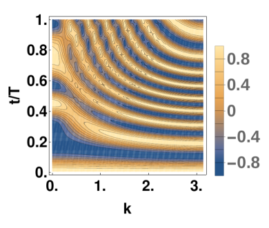
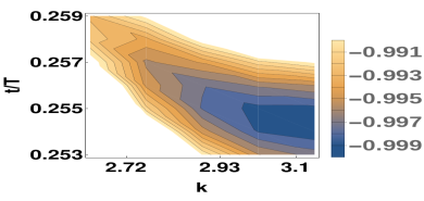
Figure 3: Left Panel: Plot of $\cos(\phi_{k}(t))$ as a function of $k$ and $t/T$ for the ID Ising model with $\omega_{D}=0.25$. All other parameters are the same as in Fig. 2. Right Panel: A close-up of $\cos\phi_{k}(t)$ showing a phase-band crossing at $k=\pi$ and $t/T\simeq 0.245$. All parameters are the same as those in the left panel.

II.2 Phase band crossing conditions

The phase bands $\lambda_{{\vec{k}}\pm}^{a}(t)=\exp[\pm i\phi^{a}_{{\vec{k}}}(t)]$ (where $a=$ I, II or III) whose expressions were obtained in Sec. II.1, cross when $\phi_{\vec{k}}^{a}(t)=n\pi$ for any integer $n$. We note that all such crossings for the integrable models that we study constitute examples of zone-edge singularities rudner1 and are therefore topologically significant. To understand when such crossings can happen, we first note that $\mu_{{\vec{k}}}(t)\leq 1$ since it denotes the overlap between ground state wave functions at different times. This property of $\mu_{{\vec{k}}}(t)$ ensures that the right hand sides of Eqs. (42), (50), and (57) can becomes unity only when $\mu_{{\vec{k}}}(t)=1\,{\rm or}\,0$. This, in turn, can occur only for momenta ${\vec{k}}={\vec{k}}_{0}$ for which $\Delta_{{\vec{k}}_{0}}=0$; thus phase band crossings only occur at these momenta.

This condition for phase band crossings happens to be a general result which may also be understood from simpler intuitive arguments. We present two such equivalent arguments here. The first of these involves a geometrical construction which invokes the concept of the Bloch sphere. Since the generators of $U_{{\vec{k}}}(t)$ belong to the SU(2) algebra, the trajectory of any wave function under its action can be considered as a trajectory on the Bloch sphere characterized by a fixed momentum ${\vec{k}}$. Thus the requirement for a phase band crossing at $U_{{\vec{k}}_{0}}(t_{0})$ amounts to the condition $|\psi_{{\vec{k}}_{0}}(0)\rangle=|\psi_{\vec{k}_{0}}(t_{0})\rangle$, i.e., the trajectory of the wave function for ${\vec{k}}={\vec{k}}_{0}$ must cross itself at $t=t_{0}$ under the action of $U_{{\vec{k}}_{0}}(t_{0})$. Since the eigenvalues of $U_{\vec{k}}(t)$ are independent of the initial wave function $|\psi_{\vec{k}}(0)\rangle$, this condition requires that the trajectory on the Bloch sphere, no matter where it starts, must pass through itself at $t=t_{0}$ during its evolution. This condition can be generically satisfied if that trajectory is generated by rotation around a single axis at all times. Thus such crossings can only occur if $\Delta_{{\vec{k}}}=0$.

The second, equivalent, argument showing that $\Delta_{{\vec{k}}}=0$ constitutes a necessary condition for phase band crossings is as follows. A Trotter decomposition of Eq. (1) enables us to write $U_{{\vec{k}}}(t)$ at the time $t_{0}$ when the phase band crosses at any given ${\vec{k}}$ as

$$U_{{\vec{k}}}(t_{0},0) = \lim_{N\to\infty}\prod_{j=0,N-1}U_{\vec{k}}(t_{j+1},t_{j})$$

$$= \lim_{N\to\infty}\prod_{j=\ell+1,N-1}U_{{\vec{k}}}(t_{j+1},t_{j})\prod_{j=0,\ell}U_{{\vec{k}}}(t_{j+1},t_{j}),$$

where $t_{j}-t_{j-1}=\Delta t=t_{0}/N$, $t_{0}=t_{N}$, and in the second line we have organized the product into two groups for which $t_{j}\leq t_{\ell}$ and $t_{j}>t_{\ell}$. Note that the choice of $t_{\ell}$ is completely arbitrary. Now since the product of these evolution matrices in each of the two groups must also be a SU(2) rotation matrix, we can write

$$U_{{\vec{k}}}(t_{0},0) = U_{2\vec{k}}(t_{0},t_{\ell+1})U_{1{\vec{k}}}(t_{\ell+1},0)$$ (60)

$$= e^{-i(\vec{\sigma}\cdot{\vec{n}}_{2{\vec{k}}})\phi_{2{\vec{k}}}}e^{-i(\vec{\sigma}\cdot{\vec{n}}_{1{\vec{k}}})\phi_{1{\vec{k}}}},$$

where ${\vec{n}}_{1(2){\vec{k}}}$ are unit vectors and $\phi_{1(2){\vec{k}}}$ are rotation angles. All of these parameters depend, in general, on the choice of $t_{\ell}$, the details of $H_{{\vec{k}}}(t)$, and the drive protocol. We do not attempt to compute them here; instead, we merely observe that in order to get $U_{{\vec{k}}}(t_{0})=I$ independent of the choice of $t_{\ell}$, we clearly require ${\vec{n}}_{2{\vec{k}}}={\vec{n}}_{1{\vec{k}}}$. This is most easily seen by choosing $n_{1\vec{k}}=\hat{z}$ which can be done without loss of generality by choosing suitable axes, and then checking that the eigenvalues of $U_{\vec{k}}$ can never be unity if $n_{2\vec{k}}\neq\hat{z}$. Next we note that the condition $n_{2\vec{k}}=n_{1\vec{k}}$ can only be satisfied for arbitrary $t_{\ell}$ if $U_{{\vec{k}}}(t_{i})$ commutes at all $t_{i}$, i.e., if the rotation axis of $U_{{\vec{k}}}(t_{j+1},t_{j})$ is the same for all $t_{j}$. In the context of the Hamiltonian $H_{{\vec{k}}}(t)$ given in Eq. (4), this is only possible if $\Delta_{{\vec{k}}}=0$. In a more general context, the Hamiltonian of the system can be written as

$$H_{{\vec{k}}}(t) = \sum_{i=1}^{3}\tau_{i}f_{i{\vec{k}}}(t),$$ (61)

where $f_{i\vec{k}}(t)$ are parameter functions and the Pauli matrices $\tau_{i}$ are the generators. The condition for the phase band crossings requires that any two of the three parameter functions $f_{i{\vec{k}}}(t)$ vanishes at all times. The third parameter function then determines $t_{0}$, and we discuss this issue in detail below. Finally, we note that the above mentioned arguments indicate that for arbitrary single-rate protocols and for $d=1$, the phase band crossings can therefore only occur at $k=0$ or $\pi$. In contrast, for $d>1$ systems such crossings can occur for a wider range of momenta.

Next, we chart out the condition for phase band crossing at ${\vec{k}}={\vec{k}}_{0}$ which yields the band crossing time $t_{0}$ for each of the regions shown in Fig. 1. In region I, we find from Eqs. (24) and (42) that the phase bands will cross at time $t_{0}<t_{1{\vec{k}}_{0}}$ provided that

$$\xi_{{\vec{k}}_{0}}(t_{0},0)=n\pi,\quad n\in Z.$$ (62)

To find the condition for phase band crossings in region II, we need to find $p_{{\vec{k}}_{0}}$. Since at ${\vec{k}}={\vec{k}}_{0}$, $\Delta_{\vec{k}_{0}}=0$, $p_{{\vec{k}}_{0}}$ may assume the values $1$ or $0$. The former occurs at the critical mode where the instantaneous energy levels of $H$ cross while for the latter they do not cross. In what follows, we denote the momenta of the critical modes to be ${\vec{k}}_{0}$ and for that of the non-critical modes to be ${\vec{k}}^{\prime}_{0}$. Within our convention, in $d=1$, $k_{0}=0$ and $k^{\prime}_{0}=\pi$. For the critical modes, the crossing of the instantaneous energy levels ensures that there is no overlap of the instantaneous ground state wave function in region II with the initial ground state wave function. This corresponds to $\mu_{{\vec{k}}_{0}}(t)=0$ and leads to $\phi_{\vec{k}_{0}}^{II}(t)=\zeta^{II}_{2{\vec{k}}_{0}}(t)$. Thus using Eqs. (48) and (50), we obtain

$$\xi_{{\vec{k}}_{0}}(t_{1{\vec{k}}_{0}},0)-\xi_{{\vec{k}}_{0}}(t_{0},t_{1{\vec{k}}_{0}}) = n\pi.$$ (63)

For the non-critical momenta $k^{\prime}_{0}$, when the instantaneous energy bands do not cross even though $\Delta_{k^{\prime}_{0}}$ vanishes, $p_{\vec{k}^{\prime}_{0}}=0$ and $\mu_{{\vec{k}}^{\prime}_{0}}(t)=1$ in region II. Using Eq. (50), we find that in this case $\phi_{{\vec{k}}^{\prime}_{0}}^{II}(t)=\zeta^{II}_{1{\vec{k}}^{\prime}_{0}}(t)$, and the phase bands cross if Eq. (62) holds, with $t_{1{\vec{k}}_{0}}\leq t_{0}\leq t_{2{\vec{k}}_{0}}$.

Finally, we obtain the conditions for such band crossings in region III. In this case, since the critical point is crossed again, $\mu_{{\vec{k}}}(t)=1$ for all ${\vec{k}}={\vec{k}}_{0},{\vec{k}}^{\prime}_{0}$. For the critical modes, where $p_{{\vec{k}}_{0}}=1$, using Eqs. (24) and (57), we find

$$\xi_{{\vec{k}}_{0}}(t_{1{\vec{k}}_{0}},0)-\xi_{{\vec{k}}_{0}}(t_{2\vec{k}_{0}},t_{1{\vec{k}}_{0}})+\xi_{{\vec{k}}_{0}}(t_{0},t_{2{\vec{k}}_{0}})=n\pi.$$ (64)

For the non-critical modes, where the instantaneous energy levels do not cross at $t_{1{\vec{k}}}$ or $t_{2{\vec{k}}}$, $p_{{\vec{k}}^{\prime}_{0}}=0$ and we find from Eq. (57) that the crossing condition is given by Eq. (62) with $t_{0}\geq t_{2{\vec{k}}}$.

Eqs. (62), (63) and (64) constitute general conditions for phase band crossings for the integrable models that we study. Although we have obtained them using the adiabatic-impulse approximation, they are essentially exact since the adiabatic-impulse approximation becomes exact for modes for which $\Delta_{{\vec{k}}_{0}}=0$. Our results also demonstrate that the conditions for the phase band crossings at the critical mode (Eqs. (63) and (64)), where we find an unavoided crossing of the instantaneous energy levels, is different from those of the non-critical modes with no instantaneous energy level crossings. The origin of this difference can be easily traced to the fact that at each such crossing $g(t)-b_{{\vec{k}}_{0}}$ changes sign; thus the sign of the phase accumulated is reversed in region II which leads to the difference between Eqs. (63) and (64) with Eq. (62). We also note that the difference in phase band crossing conditions for the critical modes that we unravel here is absent for all protocols where the critical point/region is traversed instantly, i.e., at an infinite rate. Examples of such protocols include periodic arrays of $\delta$-function kicks and square pulses studied earlier thakurathi1 ; thakurathi2 ; rudner1 ; for these protocols $t_{2\vec{k}}=t_{1{\vec{k}}}$ for all ${\vec{k}}$. Consequently Eqs. (63) and (64) become identical to Eq. (62).

Having established the crossing conditions for a generic protocol, we now study specific examples of such crossing for the 1D transverse field Ising model and the 2D Kitaev model. For the transverse field Ising model, the crossings occur at $k=0$ or $k=\pi$. For the latter mode, there is no band crossing and the crossing condition is given by Eq. (62), while for the former mode, the bands cross when $h(t)=1$ and the crossing conditions in regions II and III are given by Eqs. (63) and (64). Using the protocol $h(t)=h_{0}+h_{1}\cos(\omega_{D}t)$, we find that the band crossing conditions at $k=\pi$ in all three regions is given by

$$h_{1}\sin(x)+(h_{0}+1)x = n\pi\omega_{D},$$ (65)

where $x=\omega_{D}t$ and $n$ is an integer. For the $k=0$ mode, the conditions in region I, II and III can be obtained from Eqs. (62), (63) and (64). Noting that $E_{0}(t)=|h(t)-1|$ and $h(t)-1$ changes sign at $t_{1}$ and $t_{2}$, we can combine the conditions in Eqs. (62), (63), and (64) to obtain

$$h_{1}\sin(x)+(h_{0}-1)x = n\pi\omega_{D}.$$ (66)

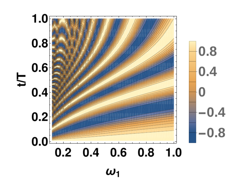
Figure 5: A plot of $\cos(\phi_{\pi}(t))$ as a function of $\omega_{D}$ and $t/T$ for the 1D transverse field Ising model for the drive protocol $h(t)=h_{0}+h_{1}\cos(\omega_{D}t)$ with $h_{0}=1.1$, and $h_{1}=-1$. Note that in contrast to Fig. 4, the phase band crossings (bright yellow regions) depend on $\omega_{D}$.

We note that for $n=0$, the crossing conditions imply that $\omega_{D}t_{0}$ is constant which indicates that such a crossing spans over a range of frequencies. This observation is verified from the plot of the phase bands at $k=0$ as a function of $\omega_{D}$ and $t/T$. We find that the crossing time $t/T$ corresponding to $\phi_{0}(t_{0})=0$ which occurs in region II is independent of $\omega_{D}$; thus $\cos[\phi_{0}(t)]=1$ for any $\omega_{D}$ at $t_{0}/T=0.45$ as can be seen in Fig. 4. A similar plot for $k=\pi$ (Fig. 5) does not show this behavior; for $k=\pi$ and for our choice of $h_{0}$ and $h_{1}$ the crossing always occur at $n\neq 0$ (Eq. (65)).

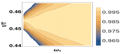
Figure 4: Left Panel: A plot of $\cos(\phi_{0}(t))$ as a function of $\omega_{D}$ and $t/T$ for the 1D transverse field Ising model for the drive protocol $h(t)=h_{0}+h_{1}\cos(\omega_{D}t)$, with $h_{0}=1.1$, and $h_{1}=-1$. Note the extended region around $t/T=0.45$ where $\phi_{0}(t)$ vanishes independently of the value of $\omega_{D}$. See text for details. Right Panel: A closer look at a phase band crossing corresponding to $n=1$ highlighting the local nature of the crossing as a function of $t/T$ and $\omega_{D}$.

Next, we consider the Kitaev model in $d=2$. kit1 ; nussinov1 This model consists of spin-1/2’s on a honeycomb lattice with nearest-neighbor interactions described by the Hamiltonian

$$H = \sum_{j+l={\rm even}}\left(J_{1}\sigma_{j+1,l}^{x}\sigma_{j,l}^{x}~{}+~{}J_{2}\sigma_{j-1,l}^{y}\sigma_{j,l}^{y}\right.$$ (67)

$$~{}~{}~{}~{}~{}~{}~{}~{}~{}~{}~{}~{}~{}~{}~{}~{}\left.+~{}J_{3}\sigma_{j,l+1}^{z}\sigma_{j,l}^{z}\right),$$

where $(j,l)$ denotes coordinates of a site on the honeycomb lattice, and $J_{1,2,3}$ are the couplings between the $x,y,z$ components of neighboring spins. The unit cell of the system has two sites which we label as $a$ and $b$. Denoting the location of a unit cell by ${\vec{n}}$, a Jordan-Wigner transformation takes us from spin-1/2’s to two Hermitian (Majorana) fermion operators in each unit cell labeled as $a_{\vec{n}}$ and $b_{\vec{n}}$. We can go to momentum space by defining

$$a_{\vec{n}} = \sqrt{\frac{4}{N}{}}~{}\sum_{\vec{k}}~{}[a_{\vec{k}}~{}e^{i{\vec{k}}\cdot{\vec{n}}}~{}+~{}a_{\vec{k}}^{\dagger}~{}e^{-i{\vec{k}}\cdot{\vec{n}}}],$$

$$b_{\vec{n}} = \sqrt{\frac{4}{N}{}}~{}\sum_{\vec{k}}~{}[b_{\vec{k}}~{}e^{i{\vec{k}}\cdot{\vec{n}}}~{}+~{}b_{\vec{k}}^{\dagger}~{}e^{-i{\vec{k}}\cdot{\vec{n}}}],$$ (68)

where $N$ is the number of sites (the number of unit cells is $N/2$), and the sum over ${\vec{k}}$ goes over half the Brillouin zone. A convenient choice of the Brillouin zone is given by a rhombus whose vertices lie at $(k_{x},k_{y})=(\pm 2\pi,0)$ and $(0,\pm 2\pi/\sqrt{3})$; half the Brillouin zone is then an equilateral triangle with vertices at $(0,\pm 2\pi/\sqrt{3})$ and $(2\pi,0)$.

Eq. (67) leads to a fermionic Hamiltonian of the form

$$H = \sum_{\vec{k}}~{}\left(\begin{array}[]{cc}a_{\vec{k}}^{\dagger}&b_{\vec{k}}^{\dagger}\end{array}\right)~{}H_{\vec{k}}~{}\left(\begin{array}[]{c}a_{\vec{k}}\\ b_{\vec{k}}\end{array}\right),$$ (72)

$$H_{\vec{k}} = 2[J_{1}\sin({\vec{k}}\cdot\vec{M}_{1})-J_{2}\sin({\vec{k}}\cdot\vec{M}_{2})]\tau^{x}$$ (73)

$$+2[J_{3}+J_{1}\cos({\vec{k}}\cdot\vec{M}_{1})+J_{2}\cos({\vec{k}}\cdot\vec{M}_{2})]\tau^{y},$$

where $\vec{M}_{1}=\frac{1}{2}\hat{i}+\frac{\sqrt{3}}{2}\hat{j}$ and $\vec{M}_{2}=\frac{1}{2}\hat{i}-\frac{\sqrt{3}}{2}\hat{j}$ are spanning vectors which join some neighboring unit cells ($\hat{i}$ and $\hat{j}$ denote unit vectors in the $x$ and $y$ directions, and we have taken the nearest-neighbor spacing to be equal to $1/\sqrt{3}$), and $\tau^{a}$ are Pauli matrices in the $a,~{}b$ space.

We now drive $J_{3}$ is periodically in time as

$$J_{3}(t)~{}=~{}h_{0}~{}+~{}h_{1}\cos(\omega_{D}t).$$ (74)

To see what happens to the phase bands, let us consider the case $J_{1}=J_{2}$ for simplicity. We then obtain

$$H_{\vec{k}} = 4J_{1}\cos(k_{x}/2)\sin(\sqrt{3}k_{y}/2)\tau^{x}$$ (75)

$$+[2J_{3}(t)+4J_{1}\cos(k_{x}/2)\cos(\sqrt{3}k_{y}/2)]\tau^{y}.$$

The form of this is similar to that in Eq. (4), except that $\tau^{z}$ has been replaced by $\tau^{y}$; indeed these two Hamiltonians are related to each other by a global unitary transformation ks1 . By the arguments given earlier, we therefore see that phase band crossings will occur at a momentum ${\vec{k}}_{0}$ and time $t_{0}$ given by

$$\cos(k_{0x}/2)\sin(\sqrt{3}k_{0y}/2) = 0,$$ (76)

$$(h_{0}+2J_{1}\cos(\frac{k_{0x}}{2})\cos(\frac{\sqrt{3}k_{0y}}{2}))x+h_{1}\sin(x) = \frac{n\pi\omega_{D}}{2},$$

where $x=\omega_{D}t_{0}$. We now observe that the first equation in Eq. (76) is satisfied for momenta lying on one of two lines in half the Brillouin zone; the two lines are given by

(i) $k_{0x}=\pi$ and $-\pi/\sqrt{3}\leq k_{0y}\leq\pi/\sqrt{3}$,
(ii) $k_{0y}=0$ and $0\leq k_{0x}\leq 2\pi$.

Correspondingly, the second equation in Eq. (76) implies that we must have

$$h_{0}x~{}+~{}h_{1}\sin(x)~{}=~{}\frac{n\pi\omega_{D}}{2}$$ (77)

on line (i), and

$$(h_{0}+2J_{1}\cos(k_{0x}/2))x~{}+~{}h_{1}\sin(x)~{}=~{}\frac{n\pi\omega_{D}}{2}$$ (78)

on line (ii). Interestingly, Eqs. (77-78) show that the phase band crossing time $t_{0}$ is independent of the location of the momentum on line (i) but depends on the location of the momentum $k_{0x}$ on line (ii). Analogous conditions for the case $J_{1}\neq J_{2}$ can be obtained by a similar analysis of Eq. (75); however analytical expressions similar to Eq. (76) may be difficult to obtain in such cases.

To conclude, in the 2D Kitaev model, phase band crossings occur on certain lines in momentum space. This is in contrast to 1D models like the Ising model in a transverse field where phase band crossings occur only at some discrete momenta, namely, 0 and $\pi$. This difference constitute a concrete example of the symmetry based arguments provided in Ref. rudner1, .

III Fermionic correlators

In this section, we show that the phase band crossings leave their imprint on the Fourier transform of some of the off-diagonal fermionic correlators. To this end, we recall that the time-dependent Hamiltonians $H$ given by Eqs. (3) and (4). Here and in the rest of this section, we shall assume $\Delta_{\vec{k}}$ to be real for simplicity; however our analysis may be readily generalized to complex $\Delta_{{\vec{k}}}$. To obtain the correlators, we first note that if $(u_{{\vec{k}}},v_{{\vec{k}}})^{T}$ is an eigenvector of $H_{\vec{k}}$, the eigenstates of $H_{{\vec{k}}}$ in second quantized form is given by $(u_{{\vec{k}}}+v_{{\vec{k}}}c_{\vec{k}}^{\dagger}c_{-{\vec{k}}}^{\dagger})|vac\rangle$. In this state, we find that $\langle c_{{\vec{k}}}^{\dagger}c_{{\vec{k}}}\rangle=\langle c_{-{\vec{k}}}^{\dagger}c_{-{\vec{k}}}\rangle=|v_{{\vec{k}}}|^{2}$ and $\langle c_{{\vec{k}}}^{\dagger}c_{-{\vec{k}}}^{\dagger}\rangle=u_{{\vec{k}}}v_{{\vec{k}}}^{*}$. In what follows, we rewrite the expressions for these correlators in a different way so as to point out their connections to the phase bands. To do this, let us denote the eigenvectors of $U_{{\vec{k}}}(t)$ corresponding to the eigenvalues $\lambda_{\pm{\vec{k}}}(t)=\exp[i\phi_{\pm{\vec{k}}}(t)]=\exp[\pm i\phi_{{\vec{k}}}(t)]$ as

$$|\chi_{\pm{\vec{k}}}(t)\rangle=\left(\begin{array}[]{c}\mu_{\pm\vec{k}}(t)\\ \nu_{\pm{\vec{k}}}(t)\end{array}\right).$$ (81)

Note that $|\chi_{\pm{\vec{k}}}(t)\rangle$ forms a complete basis. Using these eigenvectors and eigenvalues, we can now generic expressions for both the off-diagonal and the diagonal correlators in terms of these eigenvectors and eigenvalues as

$$C_{{\vec{k}}}(t) = \langle\psi_{{\vec{k}}}(0)|U^{\dagger}_{{\vec{k}}}(t)c_{{\vec{k}}}^{\dagger}c_{{\vec{k}}}U_{{\vec{k}}}(t)|\psi_{{\vec{k}}}(0)\rangle$$

$$= \sum_{a,b=\pm}(u^{0}_{{\vec{k}}}\mu_{a{\vec{k}}}(t)+v_{{\vec{k}}}^{0}\nu_{a{\vec{k}}}(t))\nu^{\ast}_{a{\vec{k}}}(t)\nu_{b{\vec{k}}}(t)$$

$$\times e^{-i(\phi_{a{\vec{k}}}(t)-\phi_{b{\vec{k}}}(t))}(u^{0}_{\vec{k}}\mu_{b{\vec{k}}}(t)+v_{{\vec{k}}}^{0}\nu_{b{\vec{k}}}(t)),$$

$$F_{{\vec{k}}}(t) = \langle\psi_{{\vec{k}}}(0)|U^{\dagger}_{{\vec{k}}}(t)c^{\dagger}_{-{\vec{k}}}c^{\dagger}_{{\vec{k}}}U_{{\vec{k}}}(t)|\psi_{\vec{k}}(0)\rangle$$ (82)

$$= \sum_{a,b=\pm}(u^{0}_{{\vec{k}}}\mu_{a{\vec{k}}}(t)+v_{{\vec{k}}}^{0}\nu_{a{\vec{k}}}(t))\mu^{\ast}_{a{\vec{k}}}(t)\nu_{b{\vec{k}}}(t)$$

$$\times e^{-i(\phi_{a{\vec{k}}}(t)-\phi_{b{\vec{k}}}(t))}(u^{0}_{\vec{k}}\mu_{b{\vec{k}}}(t)+v_{{\vec{k}}}^{0}\nu_{b{\vec{k}}}(t)).$$

Thus we find that the phase bands contribute to the terms in the correlators for $a\neq b$. For ${\vec{k}}={\vec{k}}_{0}$, for which $|\chi_{\pm{\vec{k}}}(t)\rangle$ are eigenstates of $\tau_{z}$ at all times, time-dependent contributions from the phase bands only appear in $F_{{\vec{k}}}(t)$, since $C_{{\vec{k}}}(t)$ receives contribution only from the $a=b$ terms which are time-independent. Finally, we note that for $d=1$ where the phase bands cross at $k=0,\pi$, where $c_{k_{0}}^{\dagger}c_{-k_{0}}^{\dagger}=0$ due to Pauli exclusion; however these correlators are non-zero for $d>1$ where such crossing may occur at ${\vec{k}}_{0}\neq 0,\pi$.

For ${\vec{k}}={\vec{k}}_{0}$, the phase bands are given by $\phi_{\pm{\vec{k}}_{0}}(t)=\pm\int_{0}^{t}dt^{\prime}(g(t^{\prime})-b_{{\vec{k}}_{0}})$, and the corresponding eigenvectors are $|\chi_{+\vec{k}_{0}}(t)\rangle=(1,0)^{T}$ and $|\chi_{-{\vec{k}}_{0}}(t)\rangle=(0,1)^{T}$. Substituting these in Eq. (82), we obtain $C_{{\vec{k}}_{0}}(t)=|v^{0}_{{\vec{k}}_{0}}|^{2}$ (which is independent of time) and

$$F_{{\vec{k}}_{0}}(t)=u_{{\vec{k}}_{0}}^{0}v_{{\vec{k}}_{0}}^{0\ast}\exp[-2i\int_{0}^{t}dt^{\prime}(g(t^{\prime})-b_{{\vec{k}}_{0}})].$$ (83)

We note that if the phase bands cross at $t=t_{0}$, we have $F_{\vec{k}_{0}}(t_{0})=F_{{\vec{k}}_{0}}(0)=u_{{\vec{k}}_{0}}^{0}v_{{\vec{k}}_{0}}^{0}$. In what follows, we study the Fourier transform of these correlators given by

$$F_{{\vec{k}}_{0}}(\omega_{0})=\int_{0}^{T}dte^{i\omega_{0}t}F_{{\vec{k}}_{0}}(t),$$ (84)

and show that the phase band crossings leave their imprint on the Fourier transform.

For the sake of concreteness, we apply these ideas to the Kitaev model with the Hamiltonian given in Eq. (75). As remarked earlier, the structure of this is similar to (3) except that $\tau^{y}$ is replaced by $\tau^{z}$, and the Kitaev model has an off-diagonal couplings like $a_{\vec{k}}^{\dagger}b_{\vec{k}}$ (which conserve fermion number) instead of superconducting pairing terms like $c_{\vec{k}}^{\dagger}c_{-{\vec{k}}}^{\dagger}$. We can take care of this difference by transforming to the basis of $\tau^{y}$ given by

$$c_{\vec{k}}~{}=~{}\frac{1}{\sqrt{2}}~{}(a_{\vec{k}}+ib_{\vec{k}}),~{}~{}~{}~{}d_{\vec{k}}~{}=~{}\frac{1}{\sqrt{2}}~{}(a_{\vec{k}}-ib_{\vec{k}}).$$ (85)

At time $t=0$, we take the wave function to be $(u_{{\vec{k}}}^{0},v_{{\vec{k}}}^{0})^{T}$ which denotes the state $(u_{{\vec{k}}}^{0}c_{\vec{k}}^{\dagger}+v_{{\vec{k}}}^{0}d_{\vec{k}}^{\dagger})|vac\rangle$ in second quantized notation. We can then calculate the time-dependent fermionic correlators in the Kitaev model in the same way as in the previous paragraph.

For the drive protocol given in Eq. (74), we have seen that phase band crossings can occur when the term proportional to $\tau^{x}$ in Eq. (75) vanishes, and these happens on one of two lines in momentum space. For definiteness, let us consider a point ${\vec{k}}_{0}$ on the second line, with $k_{0y}=0$ and $0\leq k_{0x}\leq 2\pi$. Using Eq. (82) and (83), we then find that $\langle c_{{\vec{k}}_{0}}^{\dagger}c_{{\vec{k}}_{0}}\rangle_{t}$ and $\langle d_{{\vec{k}}_{0}}^{\dagger}d_{{\vec{k}}_{0}}\rangle_{t}$ are independent of time. In contrast the off-diagonal correlator is given by $F_{{\vec{k}}}(t)=\langle c_{{\vec{k}}}^{\dagger}d_{{\vec{k}}}\rangle_{t}$ and reads

$$F^{(1)}_{{\vec{k}}_{0}}(t) = u_{0}^{*}v_{0}\exp[-i\omega_{{\vec{k}}_{0}}t+i(4h_{1}/\omega_{D})\sin(\omega_{D}t)],$$

$$\omega_{{\vec{k}}_{0}} = -4h_{0}-8J_{1}\cos(k_{0x}/2)$$ (86)

The Fourier transform of (86) for one time period $T$ is given by

$$F^{(1)}_{{\vec{k}}_{0}}(\omega_{0})~{}=~{}-iu_{0}^{*}v_{0}\sum_{n=-\infty}^{\infty}J_{n}\left(\frac{4h_{1}}{\omega_{D}}\right)~{}\frac{e^{i(\omega-\omega_{{\vec{k}}_{0}}+n\omega_{D})T}~{}-~{}1}{\omega-\omega_{{\vec{k}}_{0}}+n\omega_{D}},$$ (87)

where we have used the identity abram

$$e^{iz\sin\theta}~{}=~{}\sum_{n=-\infty}^{\infty}~{}J_{n}(z)~{}e^{in\theta}.$$ (88)

If $4h_{1}/\omega_{D}\ll 1$, the $n=0$ term will dominate in the sum in Eq. (87). We then find that as a function of $\omega$, the magnitude of $F^{(1)}_{{\vec{k}}_{0}}(\omega)$ has a maximum at $\omega_{0}\simeq\omega_{{\vec{k}}_{0}}$ where $|F^{(1)}_{{\vec{k}}_{0}}(\omega_{0})|\simeq|u_{0}^{*}v_{0}TJ_{0}(4h_{1}/\omega_{D})|$, and minima at $\omega_{0m}\simeq\omega_{{\vec{k}}_{0}}+m\omega_{D}$ (with $m$ being a non-zero integer) where $F^{(1)}_{{\vec{k}}_{0}}(\omega_{0m})=0$. Since the phase band crossings occur at times $t_{0}$ given by $\omega_{{\vec{k}}_{0}}t_{0}-(4h_{1}/\omega_{D})\sin(\omega_{D}t_{0})=2p\pi$ (where $p\in Z$), we therefore obtain that $F^{(1)}_{{\vec{k}}_{0}}(\omega_{0})$ will be maximum if

$$\omega_{0}t_{0} = (4h_{1}/\omega_{D})\sin[\omega_{D}t_{0}]+2\pi p,$$ (89)

and display minima at

$$\omega_{0m}t_{0} = (4h_{1}/\omega_{D})\sin[\omega_{D}t_{0}]+m\omega_{D}t_{0}+2\pi p$$ (90)

for non-zero integer $m$. Thus the maxima-minima pattern of $F^{(1)}_{\vec{k}_{0}}(\omega_{0})$ contains information about the phase band crossing time. The precise relation between $t_{0}$, $\omega_{D}$ and $\omega_{0}$ which leads to these maxima and minima depends on the drive protocol used. This is demonstrated in Fig. 6 where $|F_{\vec{k}_{0}}^{(1)}(\omega)|$ is plotted as a function of the frequency $\omega$ in the left panel; the right panel shows the position of $t_{0}$ as obtained from Eqs. (77) and (78) for the specific drive parameters used. We note that the maxima and the minima of $|F_{\vec{k}_{0}}^{(1)}(\omega)|$ occurs at frequencies which are given by Eq. (89) and (90) with $t_{0}=0.4T$.

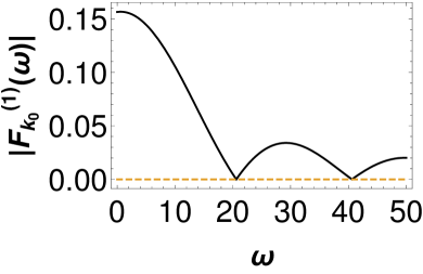
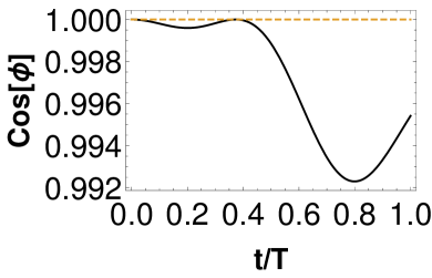
Figure 6: Left Panel: Plot of $|F^{(1)}_{\bf k_{0}}(\omega_{0})|$ vs $\omega_{0}$ for the Kitaev model showing maxima and minima of the off-diagonal correlation function with $(k_{x0},k_{y0})=(\pi/9,0)$. The protocol used is $J_{3}(t)=h_{0}+h_{1}\cos(\omega_{D}t)$ with $h_{0}=h_{1}=0.5$, and $\omega_{D}=20$. Here we have chosen $u_{0}=v_{0}=1/\sqrt{2}$, $J_{1}=J_{2}$, and all energies are scaled in units of $J_{1}$. The right panel shows that phase bands cross at $t_{0}=0.4T$; we find that the maxima and minima obtained coincides with those predicted from Eqs. (89) with $p=0$ (maxima) and Eq. (90) with $p=0$ and $m=1,2$ (minima). The dotted lines are guides to the eye.

To elucidate the protocol dependence stated above, we consider a drive protocol consisting of periodic $\delta$-function kicks thakurathi2 ,

$$J_{3}(t)~{}=~{}h_{0}~{}+~{}h_{1}~{}\sum_{n=-\infty}^{\infty}~{}\delta(t-nT),$$ (91)

for which the phase band crossings occur at $\omega_{{\vec{k}}_{0}}t_{0}-4h_{1}=2n\pi$, where $\omega_{{\vec{k}}_{0}}$ is given in Eq. (86). A calculation similar to the one outlined above yields

$$F^{(2)}_{{\vec{k}}_{0}}(\omega)~{}=~{}-iu_{0}^{*}v_{0}~{}e^{i4h_{1}}~{}\frac{e^{i(\omega-\omega_{{\vec{k}}_{0}})T}~{}-~{}1}{\omega-\omega_{{\vec{k}}_{0}}}.$$ (92)

The magnitude of $F^{(2)}_{{\vec{k}}_{0}}(\omega_{0})$ has a maximum at $\omega_{0}=\omega_{{\vec{k}}_{0}}$ where $|F^{(2)}_{vk_{0}}(\omega_{0})|=|u_{0}^{*}v_{0}T|$, and minima at $\omega_{0m}=\omega_{{\vec{k}}_{0}}+m\omega_{D}$ (with $m\neq 0$) where $F^{(2)}_{{\vec{k}}_{0}}(\omega_{0m})=0$. This leads to the relations

$$\omega_{0}t_{0}=4h_{1}+2\pi n$$ (93)

for maxima, and

$$\omega_{0m}t_{0}=4h_{1}+2\pi n+m\omega_{D}$$ (94)

for minima of $F^{(2)}_{{\vec{k}}_{0}}(\omega_{0})$.

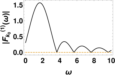
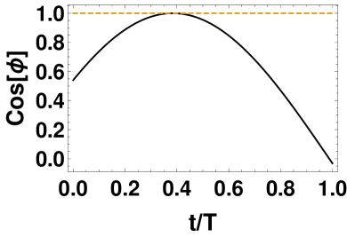
Figure 7: Left Panel: Plot of $|F^{(2)}_{\bf k_{0}}(\omega_{0})|$ vs $\omega_{0}$ for the Kitaev model showing maxima and minima of the off-diagonal correlation function for a delta function protocol with periodic kicks with $(k_{x0},k_{y0})=(\pi/2,0)$, $h_{0}=1$ and $h_{1}=0.5$. All other parameters are the same as in Fig. 6. The right panel shows that $t_{0}=0.41T$; we find that the maxima and minima obtained coincides with those predicted from Eqs. (93) with $n=0$ (maxima) and Eq. (94) with $n=0$ and $m=1,2,3$ (minima). The dotted lines are guides to the eye.

A plot of $|F_{\vec{k}_{0}}^{(2)}(\omega)|$ is plotted as a function of the frequency $\omega$ in the left panel; the right panel shows the position of $t_{0}$ for the specific drive parameters used. We note that the maxima and the minima of $|F_{\vec{k}_{0}}^{(1)}(\omega)|$ occurs at frequencies which are given by Eq. (93) and (94) with $t_{0}=0.41T$.

Before ending this section, we note that the fermionic correlators in the Kitaev model can be related to the correlators of the spins appearing in the Hamiltonian in Eq. (67).ks1 For two neighboring sites given by $b$ located at ${\vec{n}}$ and $a$ located at ${\vec{n}}+\vec{r}$ (where $\vec{r}$ can take three possible values given by $(0,0)$, $-{\vec{M}}_{1}$ and ${\vec{M}}_{2}$), we can use Eq. (68) to relate the fermionic correlators in real and momentum space,

$$\langle ib_{\vec{n}}a_{{\vec{n}}+\vec{r}}\rangle_{t}~{}=~{}\frac{i4}{N}~{}\sum_{\vec{k}}~{}\langle b_{\vec{k}}^{\dagger}a_{\vec{k}}e^{i{\vec{k}}\cdot\vec{r}}~{}-~{}a_{\vec{k}}^{\dagger}b_{\vec{k}}e^{-i{\vec{k}}\cdot\vec{r}}\rangle_{t},$$ (95)

where we have used the relations $\langle b_{\vec{k}}a_{{\vec{k}}^{\prime}}\rangle_{t}=0$ for all ${\vec{k}}$, ${\vec{k}}^{\prime}$, and $\langle b_{\vec{k}}^{\dagger}a_{{\vec{k}}^{\prime}}\rangle_{t}=0$ if ${\vec{k}}\neq{\vec{k}}^{\prime}$. Rewriting $a_{\vec{k}}$ and $b_{\vec{k}}$ in terms of $c_{\vec{k}}$ and $d_{\vec{k}}$, we find that the correlator is given by

$$\langle ib_{\vec{n}}a_{{\vec{n}}+\vec{r}}\rangle_{t} = \frac{4}{N}~{}\sum_{\vec{k}}~{}[\cos({\vec{k}}\cdot\vec{r})(\langle d_{\vec{k}}^{\dagger}d_{\vec{k}}\rangle_{t}-\langle c_{\vec{k}}^{\dagger}c_{\vec{k}}\rangle_{t})$$ (96)

$$~{}~{}~{}~{}-~{}i\sin({\vec{k}}\cdot\vec{r})(\langle c_{\vec{k}}^{\dagger}d_{\vec{k}}\rangle_{t}-\langle d_{\vec{k}}^{\dagger}c_{\vec{k}}\rangle_{t})].$$

We thus see that the terms proportional to $\sin({\vec{k}}\cdot\vec{r})$ are related to the off-diagonal fermion correlators. Next, we note that for $\vec{r}=(0,0)$, $-{\vec{M}}_{1}$ and ${\vec{M}}_{2}$, $ib_{\vec{n}}a_{{\vec{n}}+\vec{r}}$ are given by $\sigma^{z}_{b,{\vec{n}}}\sigma^{z}_{a,{\vec{n}}}$, $\sigma^{y}_{b,{\vec{n}}}\sigma^{y}_{a,{\vec{n}}-{\vec{M}}_{1}}$ and $\sigma^{x}_{b,{\vec{n}}}\sigma^{x}_{a,{\vec{n}}+{\vec{M}}_{2}}$ respectively ks1 . Hence in the last two cases, where $\vec{r}=-{\vec{M}}_{1}$ or ${\vec{M}}_{2}$, the nearest-neighbor spin correlators are related to the off-diagonal fermion correlators through Eq. (96). (If $b_{\vec{n}}$ and $a_{{\vec{n}}+\vec{r}}$ are not on nearest-neighbor sites, the relation between $ib_{\vec{n}}a_{{\vec{n}}+\vec{r}}$ and spin correlators is more complicated. Namely, $ib_{\vec{n}}a_{{\vec{n}}+\vec{r}}$ is given by a product of $\sigma^{x}$ or $\sigma^{y}$ at ${\vec{n}}$ and ${\vec{n}}+\vec{r}$ multiplied by a Jordan-Wigner string of $\sigma^{z}$’s running between those two sites).

To summarize, at the momenta ${\vec{k}}_{0}$ where phase band crossings can occur, we find that the Fourier transform of the off-diagonal correlator, $F_{{\vec{k}}_{0}}(\omega_{0})$ has maxima and minima at some particular frequencies; these frequencies are related to $\omega_{{\vec{k}}_{0}}$ (which is a function of ${\vec{k}}_{0}$) by integer multiples of the drive frequency $\omega_{D}$. The maxima and minima of these correlators provide us with a relation between $\omega_{0}$, the phase band crossing time $t_{0}$, and the drive frequency $\omega_{D}$ whose precise form depends on the drive protocol used. We note that the standard signature of the phase band crossings shows up in the form of localized subgap states at the ends of a finite sample rudner1 ; however, such a signature cannot identify the crossing time $t_{0}$ which can be done by tracking maxima and minima of $F_{{\vec{k}}_{0}}(\omega_{0})$.

IV Discussion

In this work, we have provided an analytic expression for the phase bands for a class of periodically driven integrable models for arbitrary drive protocols within the adiabatic-impulse approximation. Using this expression, and other more generic arguments, we have outlined the conditions for phase band crossings in these models for arbitrary drive protocols. As we have argued in this work, although the expressions for the phase bands are derived within the adiabatic-impulse approximation, the crossing conditions derived are exact for two reasons. First, such conditions can be derived from intuitive arguments which do not depend on the approximations used and second, the momenta at which these crossings occur are the ones in which the adiabatic-impulse approximation becomes exact. We also show that for a class of these crossings, the time of crossing $t_{0}/T$ is independent of the drive frequency $\omega_{D}$, and we provide an analytical explanation of this phenomenon. We also point out that the crossing conditions for the critical modes, where the instantaneous energy levels of the Hamiltonian undergo an unavoided level crossing, are different compared to those for the non-critical modes where no such level crossings occur. Finally, we point out that the off-diagonal fermionic correlators carry a signature of the phase band crossings, and we provide analytical relations between the frequencies $\omega_{0}$ (at which $F_{{\vec{k}}_{0}}(\omega_{0})$ either shows a maxima or vanishes), the phase band crossing time $t_{0}$, and the drive frequency $\omega_{D}$.

Our results regarding the phase band crossing conditions have some implications which we briefly discuss. First, although our results are derived for $N=2$ phase bands, they may provide an insight into generic crossing conditions for systems with $N>2$. To see this, let us consider a situation where there are $N$ phase bands for any given quasi-momentum ${\vec{k}}$ in a system. Let us consider a phase band crossing corresponding to a zone-edge singularity between the top ($N^{\rm th}$) and the bottom ($1^{\rm st}$) bands. The dynamics of these bands can always be described by an effective $2\times 2$ matrix Hamiltonian $H_{{\vec{k}}}^{\rm eff}$ which can be obtained, in principle, by integrating out all other degrees of freedom of the system Hamiltonian. Then the effective evolution operator describing the crossing of these two bands may always be written, sufficiently near the band crossing point, as $U_{{\vec{k}}}^{\rm eff}(t)={\mathcal{T}}_{t}\exp[-(i/\hbar)\int_{0}^{t}dt^{\prime}H^{\rm eff}_{{\vec{k}}}(t^{\prime})]$. The most general form of such an effective Hamiltonian is given by

$$H_{{\vec{k}}}^{\rm eff}=\sum_{i=1,3}g_{i{\vec{k}}}(t)\tau_{i},$$ (97)

where $g_{i{\vec{k}}}(t)$ are parameter functions which depend on ${\vec{k}}$ and $t$ and whose precise form depends on the details of the system Hamiltonian and the drive protocol. In terms of these $g_{i{\vec{k}}}$’s, the condition for such band crossings, as can be inferred from our results for integrable models of a similar form of $H$, is that at least two of the three $g_{i{\vec{k}}}$ (which we may choose to label as $g_{1\vec{k}}(t)$ and $g_{2{\vec{k}}}(t)$ without loss of generality) are zero for ${\vec{k}}={\vec{k}}_{0}$ and for appropriate choice of Hamiltonian parameters. The crossing time $t_{0}$ is then determined from the third generator using

$$\int_{0}^{t_{0}}dt^{\prime}g_{3{\vec{k}}_{0}}(t^{\prime})=0.$$ (98)

Our results for integrable models show that these conditions need to be satisfied for any $N$ for the system to have a band crossing corresponding to a zone-edge singularity.

The second implication of our results constitutes the relation of the symmetry classes of the underlying Hamiltonian to the condition for phase band crossings. Our results indicate that Hamiltonians belonging to the same symmetry class ryu1 and driven by identical protocols may have different behaviors of the phase bands. This becomes evident by considering the class CI which contains models of time-reversal and SU(2) symmetric superconductors that include both $d$- and $s$-wave pairing symmetries ryu1 . The Hamiltonians of such superconductors are given by Eqs. (3) and (4) where $g=-\mu_{0}$ and $b_{{\vec{k}}}=\epsilon_{\vec{k}}$, and $\mu_{0}$ and $\epsilon_{{\vec{k}}}$ are the chemical potential and energy dispersion of the fermions. For $d$-wave superconductors $\Delta_{{\vec{k}}}=\Delta_{0}(k_{x}^{2}-k_{y}^{2})/k_{F}^{2}$, while for $s-$wave $\Delta_{{\vec{k}}}=\Delta_{0}$. Now consider periodically driving such a system by changing the chemical potential: $\mu_{0}\equiv\mu_{0}(t)$. The phase bands corresponding to $U_{{\vec{k}}}(t)$ may cross at momenta given by four isolated points on the Fermi surface ${\vec{k}}_{0}=(k_{0x},k_{0y})=k_{F}(\pm 1,\pm 1)/\sqrt{2}$ for $d$-wave superconductors, while they will never cross for $s-$wave superconductors. Thus the dynamics of these two models will be very different even if they belong to the same symmetry class. Our results seem to indicate that for similar dynamics a necessary condition is that the set of zeroes of two of the parameter functions $f_{i\vec{k}}(t)$ or $g_{i\vec{k}}(t)$ defined earlier must be identical; for example, if the parameter functions never vanish so that the set of zeroes is a null set, there will be no phase band crossing for any drive protocol.

In conclusion, we have presented analytic expressions for the phase bands for a class of integrable models driven by arbitrary periodic protocols within the adiabatic-impulse approximation. Using these expression and other more general arguments, we have listed the conditions for phase band crossings for such models. We have also shown that such phase band crossings leave their mark on the Fourier transform of the off-diagonal fermionic correlators; the positions of the zeroes and maxima of such correlators provide information about the band crossing time $t_{0}$. Finally we have discussed the relevance of the derived band crossing conditions in the context of generic models with $N>2$ phase bands, and we have discussed the role of symmetry in such band crossings.

Acknowledgments

D.S. thanks DST, India for Project No. SR/S2/JCB-44/2010 for financial support.

References

- (1)
- (2) A. Polkovnikov, K. Sengupta, A. Silva, and M. Vengalattore, Rev. Mod. Phys. 83, 863 (2011).
- (3) J. Dziarmaga, Adv. Phys. 59, 1063 (2010).
- (4) A. Dutta, G. Aeppli, B. K. Chakrabarti, U. Divakaran, T. F. Rosenbaum, and D. Sen, Quantum phase transitions in transverse field spin models: from statistical physics to quantum information (Cambridge University Press, Cambridge, 2015).
- (5) L. D’Alessio, Y. Kafri, A. Polkovnikov, and M. Rigol, arXiv:1509.06411 (unpublished).
- (6) T. W. B. Kibble, J. Phys. A 9, 1387 (1976); W. H. Zurek, Nature (London) 317, 505 (1985).
- (7) A. Polkovnikov, Phys. Rev. B 72, 161201(R) (2005).
- (8) K. Sengupta, D. Sen, and S. Mondal, Phys. Rev. Lett. 100, 077204 (2008); ibid, Phys. Rev. B 78, 045101 (2008).
- (9) A. Polkovnikov, Phys. Rev. Lett. 101, 220402 (2008).
- (10) A. Chandran, A. Erez, S. S. Gubser, and S. L. Sondhi, Phys. Rev. B 86, 064304 (2012).
- (11) D. Sen, K. Sengupta, and S. Mondal, Phys. Rev. Lett. 101, 016806 (2008); ibid, 79, 045128 (2009).
- (12) F. Pollmann, S. Mukerjee, A. M. Turner, and J. E. Moore, Phys. Rev. Lett. 102 255701 (2009).
- (13) M. Heyl, A. Polkovnikov, and S. Kehrein Phys. Rev. Lett. 110, 135704 (2013).
- (14) C. Karrasch and D. Schuricht, Phys. Rev. B, 87, 195104 (2013); N. Kriel, C. Karrasch, and S. Kehrein Phys. Rev. B 90, 125106 (2014).
- (15) F. Andraschko and J. Sirker, Phys. Rev. B 89, 125120 (2014); E. Canovi, P. Werner, and M. Eckstein, Phys. Rev. Lett. 113, 265702 (2014); M. Heyl, Phys. Rev. Lett. 115, 140602 (2015).
- (16) S. Sharma, U. Divakaran, A. Polkovnikov, and A. Dutta, Phys. Rev. B 93, 144306 (2016).
- (17) A. Gambassi and A. Silva, Phys. Rev. Lett. 109, 250602 (2012).
- (18) P. Smacchia and A. Silva, Phys. Rev. E 88, 042109, (2013).
- (19) A. Das, Phys. Rev. B, 82, 172402 (2010); S. Hegde, H. Katiyar, T. S. Mahesh, and A. Das, Phys. Rev. B 90, 174407 (2014).
- (20) S. Mondal, D. Pekker, and K. Sengupta, EPL 100, 60007 (2012).
- (21) U. Divakaran and K. Sengupta, Phys. Rev. B90, 184303 (2014).
- (22) A. Lazarides, A. Das, and R. Moessner, Phys. Rev. Lett. 115, 030402 (2015).
- (23) V. Khemani, A. Lazarides, R. Moessner, and S. L. Sondhi, arXiv:1508.03344 (unpublished).
- (24) C. W. von Keyserlingk and S. L. Sondhi, arXiv:1602.02157 (unpublished); ibid, arXiv:1602.06949 (unpublished); C. W. von Keyserlingk, V. Khemani, and S. L. Sondhi, arXiv:1605.00639 (unpublished).
- (25) A. Dutta, A. Das, and K. Sengupta, Phys. Rev. E 92, 012104 (2015).
- (26) A. Sen and K. Sengupta, arXiv:1511.03668 (unpublished).
- (27) T. Kitagawa, E. Berg, M. Rudner, and E. Demler, Phys. Rev. B 82, 235114 (2010).
- (28) N. H. Lindner, G. Refael, and V. Galitski, Nat. Phys. 7, 490 (2011).
- (29) L. Jiang, T. Kitagawa, J. Alicea, A. R. Akhmerov, D. Pekker, G. Refael, J. I. Cirac, E. Demler, M. D. Lukin, and P. Zoller, Phys. Rev. Lett. 106, 220402 (2011).
- (30) Z. Gu, H. A. Fertig, D. P. Arovas, and A. Auerbach, Phys. Rev. Lett. 107, 216601 (2011).
- (31) T. Kitagawa, T. Oka, A. Brataas, L. Fu, and E. Demler, Phys. Rev. B 84, 235108 (2011).
- (32) N. H. Lindner, D. L. Bergman, G. Refael, and V. Galitski, Phys. Rev. B 87, 235131 (2013).
- (33) E. Suárez Morell and L. E. F. Foa Torres, Phys. Rev. B 86, 125449 (2012).
- (34) M. Trif and Y. Tserkovnyak, Phys. Rev. Lett. 109, 257002 (2012).
- (35) A. Russomanno, A. Silva, and G. E. Santoro, Phys. Rev. Lett. 109, 257201 (2012).
- (36) V. M. Bastidas, C. Emary, G. Schaller, and T. Brandes, Phys. Rev. A 86, 063627 (2012).
- (37) V. M. Bastidas, C. Emary, B. Regler, and T. Brandes, Phys. Rev. Lett. 108, 043003 (2012).
- (38) M. Tomka, A. Polkovnikov, and V. Gritsev, Phys. Rev. Lett. 108, 080404 (2012).
- (39) A. Gomez-Leon and G. Platero, Phys. Rev. B 86, 115318 (2012), and Phys. Rev. Lett. 110, 200403 (2013).
- (40) B. Dóra, J. Cayssol, F. Simon, and R. Moessner, Phys. Rev. Lett. 108, 056602 (2012).
- (41) D. E. Liu, A. Levchenko, and H. U. Baranger, Phys. Rev. Lett. 111, 047002 (2013).
- (42) Q.-J. Tong, J.-H. An, J. Gong, H.-G. Luo, and C. H. Oh, Phys. Rev. B 87, 201109(R) (2013).
- (43) M. S. Rudner, N. H. Lindner, E. Berg, and M. Levin, Phys. Rev. X 3, 031005 (2013).
- (44) J. Cayssol, B. Dóra, F. Simon, and R. Moessner, Phys. Status Solidi RRL 7, 101 (2013).
- (45) Y. T. Katan and D. Podolsky, Phys. Rev. Lett. 110, 016802 (2013).
- (46) A. Kundu and B. Seradjeh, Phys. Rev. Lett. 111, 136402 (2013).
- (47) V. M. Bastidas, C. Emary, G. Schaller, A. Gómez-León, G. Platero, and T. Brandes, arXiv:1302.0781v2.
- (48) T. L. Schmidt, A. Nunnenkamp, and C. Bruder, New J. Phys. 15, 025043 (2013).
- (49) A. A. Reynoso and D. Frustaglia, Phys. Rev. B 87, 115420 (2013).
- (50) C.-C. Wu, J. Sun, F.-J. Huang, Y.-D. Li, and W.-M. Liu, EPL 104, 27004 (2013).
- (51) P. M. Perez-Piskunow, G. Usaj, C. A. Balseiro, and L. E. F. Foa Torres, Phys. Rev. B 89, 121401(R) (2014).
- (52) M. Thakurathi, A. A. Patel, D. Sen, and A. Dutta, Phys. Rev. B 88, 155133 (2013).
- (53) M. Reichl and E. Mueller, Phys. Rev. A 89, 063628 (2014).
- (54) M. Thakurathi, K. Sengupta, and D. Sen, Phys. Rev. B 89, 235434 (2014).
- (55) F. Nathan and M. S. Rudner, New J. Phys. 17, 125014 (2015).
- (56) M. S. Rudner, N. H. Lindner, E. Berg, and M. Levin, Phys. Rev. X 3, 031005 (2013).
- (57) D. Carpentier, P. Delplace, M. Fruchart, and K. Gawedzki, Phys. Rev. Lett. 114, 106806 (2015).
- (58) For phase bands, the number of edge modes depends on the crossing number itself.
- (59) E. Zhao, arXiv:1603.08822v2 (unpublished).
- (60) S. Sachdev, Quantum Phase Transitions (Cambridge University Press, Cambridge, 1999).
- (61) A. Kitaev, Ann. Phys. 321, 2 (2006).
- (62) H.-D. Chen and Z. Nussinov, J. Phys. A 41, 075001 (2008).
- (63) A. H. Castro Neto, F. Guinea, N. M. R. Peres, K. S. Novoselov, and A. K. Geim, Rev. Mod. Phys. 81, 109 (2009); S. Das Sarma, S. Adam, E. H. Hwang, and E. Rossi, Rev. Mod. Phys. 83, 407 (2011); M. O. Goerbig, Rev. Mod. Phys. 83, 1193 (2011); D. N. Basov, M. M. Fogler, A. Lanzara, F. Wang, and Y. Zhang, Rev. Mod. Phys. 86, 959 (2014).
- (64) M. Z. Hasan and C. L. Kane, Rev. Mod. Phys. 82, 3045 (2010); X.-L. Qi and S.-C. Zhang, Rev. Mod. Phys. 83, 1057 (2011).
- (65) S. N. Shevchenko, S. Ashhab, and F. Nori, Phys. Reports 492, 1 (2010).
- (66) Y. Kayanuma, Phys. Rev. A 55, R2495 (1997)
- (67) M. S. Child, Molecular Collision Theory (Academic Press, London, 1974).
- (68) We consider protocols for which the slope of is the same at both crossing points for simplicity of notation. Our final results do not change for protocols where the slopes are different.
- (69) M. Abramowitz and I. A. Stegun, Handbook of Mathematical Functions (Dover, New York, 1972).
- (70) M. R. Zirnbauer, J. Math. Phys. 37, 4986 (1996); A. Altland and M. R. Zirnbauer, Phys. Rev. B 55, 1142 (1997); P. Heinzner, A. Huck Leberry, and M. R. Zirnbauer, Commun. Math. Phys. 257, 725 (2005); A. P. Schnyder, S. Ryu, A. Furusaki, and A. W. W. Ludwig, Phys. Rev. B78, 195125 (2008).