Stability of time-delay reset systems with a nonlinear and time-varying base system

Abstract

This work is devoted to investigate the stability properties of time-delay reset systems. We present a Lyapunov-Krasovskii proposition, which generalizes the available results in the literature, providing results for verifying the stability of time-delay reset systems with nonlinear and time-varying base system. We demonstrate the applicability of the proposed results in the analysis of time-delay reset control systems, and an illustrative example with nonlinear, time-varying base system.

1 Introduction

The investigation of reset systems was started more than fifty years ago with the seminal work of Clegg [1], and carried on with a series of works by Horowitz and coworkers ([2, 3]). The main motivation for the study of reset systems arises from reset control ([4]), since reset compensation may achieve fast and robust control solutions for problems under linear limitations, which as it is well-known are particularly severe in the case of control systems with time-delays ([5]). A large number of works have shown the advantages of reset control over linear control ([6, 7, 8, 4]).

The term reset system was first introduced by Hollot, Chait, and coworkers ([9]) to denote a “linear and time invariant system with (state-dependent) mechanisms and laws to reset their states to zero”. Two distinctive characteristics of reset systems are that the resetting law is state-dependent, and that (some) states are reset to zero. Therefore, reset systems can be considered as a special type of impulsive/hybrid systems, in which the system state (or a part of it) is instantaneously zeroed out at those instants in which the system solution intersects some reset set. On the other hand, time-delay systems (see the monographs [10, 11, 12], or for example the works [13, 14, 15, 16, 17]) are a natural target for reset control. As a result, time-delay reset systems have a clear interest in control practice and have been an active research topic in the last decade ([18, 19, 4]).
In addition, it should be noted that impulsive systems (without time-delays) have been a very active research topic in different areas of mathematics and systems theory ([20, 21, 22, 23]), where the research effort has been concentrated in systems with impulses at fixed/variable instants. However, as it has been discussed in ([4, 24]) reset systems (with a time invariant base system) are a special case of autonomous impulsive systems, a much less developed research topic in the literature. On the other hand, time-delay impulsive systems, or more specifically impulsive functional differential equations, have been investigated in a number of works. Again, most of the research effort has been concentrated in systems with impulses at fixed instants ([25, 26, 27, 28, 29, 30]), and to a lesser extent in systems with impulses at variable times ([31]). Note that the vast majority of stability results for impulsive functional differential equations uses Lyapunov-Razumikhin techniques (see [32] and references therein).

This work is focused on the internal stability analysis of time-delay reset systems by using a Lyapunov-Krasovskii approach, with the goal of obtaining conditions formulated by using Lyapunov-Krasovskii functionals. To the knowledge of authors, all the previous published results from the impulsive functional differential equations literature are restricted to systems with impulses at fixed times, and thus they are not applicable to our case, or are based on Lyapunov-Razumikhin techniques. In spite of that, the Lyapunov-Krasovskii approach has been already investigated in the area of reset systems; in particular, a delay-independent condition is obtained in [18] for reset control systems, and, in addition, extension to delay-dependent conditions is given in [19], and more recently in [33], considering a more general resetting law (anticipative reset). Also, quadratic stability of time-delay reset control systems with uncertainty in the resetting law has been analyzed in [34]. In general, a previous work [35] suggests that it is necessary a deeper analysis of Lyapunov-Krasovskii functionals, focusing into the necessity of obtaining less restrictive conditions. A first attempt to obtain less restrictive conditions is [35], where it has been proposed criteria based on bounded increments of the functional after the reset instants. In addition, input-output stability has been investigated in [36], based on the previous Lyapunov-Krasovskii results, and in [37], based on passivity properties of reset systems [38], and the IQC framework.

To the authors knowledge, all the previous published results are about reset systems with a linear and time-invariant (LTI) base system, and most of them are based on the existence of a Lyapunov-Krasovskii theorem; and therefore, the proof of that theorem has been only sketched, making the generalization to nonlinear and time-varying systems challenging. On the other hand, some preliminary works [39, 40, 41] have extended the hybrid inclusion model developed in [42] to investigate hybrid systems with time-delays, based on a generalized concept of solutions. In addition, the results in [40] provide sufficient conditions for the stability analysis of hybrid systems with time-delays, using Lyapunov-Razumikhin functions, but application to reset control system is still unexplored. On the other hand, although [41] approaches the case of reset systems, it deals with a restrictive class of reset systems in which the time-delay only affects a part of the state and thus its applicability is very limited in practice.

The main result of this work is the development of a Lyapunov-Krasovskii theorem for reset systems, in which the resetting law is generalized in the sense that the state may be reset to a non-zero value after a reset action, and in addition the base system is nonlinear and time-varying. In this way, this work is devoted to provide a formal and complete proof, and then to analyze reset systems with a LTI base system as a particular case. The paper is structured as follows. After formally stating the problem in Section 2, the main stability result is given in Section 3. In Section 4, two application cases of the stability result are shown; firstly, a general reset system with a LTI base system and a single time-delay; and secondly, a particular reset system with a nonlinear and time-varying base system. The work concluded in Section 5 with some final remarks.

Notation: $\mathds{R}$ is the set of real numbers, $\mathds{R}^{+}$ is the set of non-negative real numbers, $\mathds{R}^{n}$ is the n-dimensional euclidean space, where $\|\mathbf{x}\|$ is the euclidean norm for $\mathbf{x}\in\mathds{R}^{n}$, and $({\bf x},{\bf y})$, with column vectors ${\bf x}\in\mathds{R}^{n}$ and ${\bf y}\in\mathds{R}^{m}$, denotes the column vector $\left(\ {\bf x}^{\top}\ \ {\bf y}^{\top}\ \right)^{\top}$. ${\cal PC}([a,b],F)$ is the set of piecewise continuous functions from $[a,b]$ to $F$, that is the set of functions that are continuous on $[a,b]$ except in a finite number of points $(t_{k})_{k=1}^{N}$, and with a norm $\|\mathbf{\psi}\|=\sup_{\theta\in[a,b]}\|\psi(\theta)\|$. $\mathcal{R}(A)$ and $\mathcal{N}(A)$, for a matrix $A\in\mathds{R}^{n\times m}$, stand for the column space and the null space of A, respectively. $diag(A,B)$ is a block diagonal matrix composed by the matrices $A\in\mathds{R}^{n\times n}$ and $B\in\mathds{R}^{m\times m}$. For a symmetric matrix $A\in\mathds{R}^{n\times n}$, $\lambda_{m}(A)$ and $\lambda_{M}(A)$ stand for the minimum and maximum eigenvalue, respectively.

2 Preliminaries

Consider a state-dependent time-delay reset system given by the impulsive differential equation

$$\left\{\begin{array}[]{llll}\dot{\mathbf{x}}(t)=\mathbf{f}(t,\mathbf{x}_{t}),&\mathbf{x}(t)\notin{\cal M},\\ {\mathbf{x}}(t^{+})=\mathbf{I}(t,\mathbf{x}_{t}),&\mathbf{x}(t)\in{\cal M},\\ \mathbf{x}(t)=\phi(t-t_{0}),&t\in[t_{0}-h,t_{0}],\end{array}\right.$$ (1)

where $t_{0}\in\mathds{R}^{+}$ is the initial instant, $\mathbf{x}(t)\in\mathds{R}^{n}$ is the system state at the instant $t\in[t_{0}-h,\infty)$, $\mathbf{x}_{t}\in{\cal PC}([-h,0],\mathds{R}^{n})$ is the distributed state at the instant $t\in[t_{0},\infty)$, that is $\mathbf{x}_{t}(\theta)=\mathbf{x}(t+\theta)$ for $\theta\in[-h,0]$, and the initial condition is a function $\phi\in{\cal PC}([-h,0],\mathds{R}^{n})$. Henceforth, it will be denoted ${\cal PC}={\cal PC}([-h,0],\mathds{R}^{n})$ for notational simplicity. It is considered that the reset is applied at instants $t_{k}\in[t_{0},\infty)$ if $\mathbf{x}(t_{k})\in{\cal M}$, where ${\cal M}\subset\mathds{R}^{n}$ is the reset set. It is assumed that reset instants are well-posed, that is for any initial condition $\phi\in{\cal PC}$ there exists a finite or infinite sequence of well defined reset instants $\mathds{T}_{\phi}=(t_{1},t_{2},\cdots)$, such that they are distinct and satisfy $t_{0}<t_{1}<t_{2}<\cdots$; and also that reset instants are Zeno-free, that is if the reset instants sequence is infinite then $t_{N}\rightarrow\infty$ as $N\rightarrow\infty$. Otherwise, as well as in the case of free-delay impulsive dynamical systems ([22]), pathological behaviors like beating and existence of Zeno solutions may be present. A simple manner to guaranty that reset instants are well-posed and Zeno-free is to use time regularization (see for example [4]), which means that reset instants satisfy $t_{k+1}-t_{k}>\Delta$, $k=0,1,2,\ldots$, for some $\Delta>0$ (the initial instant $t_{0}$ is not a reset instant).

Thus, the existence and uniqueness of solutions of the reset system (1) follows from the existence and uniqueness of the following initial-value problem

$$\left\{\begin{array}[]{ll}\dot{{\bf z}}(t)=\mathbf{f}(t,{\bf z}_{t}),\\ {\bf z}(t)={\bf x}_{t_{k}}(t-t_{k}),&t\in[t_{k}-h,t_{k}),\\ {\bf z}(t_{k})=\mathbf{I}(t_{k},\mathbf{x}_{t_{k}}),\end{array}\right.$$ (2)

where $t\geq t_{k}$ and ${\bf x}_{t_{k}}\in\mathcal{PC}$ is the initial condition. It will be assumed that the initial value problem (2) has a unique solution for $t\geq t_{k}$ (see Corollary 3.1 in [25]). For example, that there exist constants $M$, $N\in\mathds{R}^{+}$ such that $\|\mathbf{f}(t,\psi)\|\leq M+N\|\psi\|$ for all $(t,\psi)\in\mathds{R}^{+}\times\mathcal{PC}$; and that $\mathbf{f}$ is locally Lipschitz, that is for each compact set $\Omega\subset\mathds{R}^{n}$ there exists some constant $K\in\mathds{R}^{+}$ such that $\|\mathbf{f}(t,\psi_{1})-\mathbf{f}(t,\psi_{2})\|\leq K\|\psi_{1}-\psi_{2}\|$ for all $t\in\mathds{R}^{+}$ and all $\psi_{1},\psi_{2}\in\mathcal{PC}([-h,0],\Omega)$. Thus, the initial-value problem is well-posed and for every $(t_{k},{\bf x}_{t_{k}})\in\mathds{R}^{+}\times\mathcal{PC}$, there exists a continuous and unique solution ${\bf z}(t_{k},{\bf x}_{t_{k}})(t)$ for all $t\in[t_{k},\infty)$.

Hence, the solution ${\bf x}(t_{0},\phi)$ of (1) is made up of an initial condition $\phi$ and a sequence of continuous solution segments ${\bf z}(t_{k},{\bf x}_{t_{k}})$, that is

$${\bf x}(t_{0},\phi)(t)=\left\{\begin{array}[]{ll}{\bf z}(t_{0},\phi)(t),&t\in[t_{0},t_{1}],\\ {\bf z}(t_{1},{\bf x}_{t_{1}})(t),&t\in(t_{1},t_{2}],\\ \lx@intercol\hfil\vdots\hfil\lx@intercol\\ {\bf z}(t_{k},{\bf x}_{t_{k}})(t),&t\in(t_{k},t_{k+1}].\\ \end{array}\right.$$ (3)

If the sequence of reset instants is finite then ${\bf x}(t_{0},\phi)(t)={\bf z}(t_{N},{\bf x}_{t_{N}})(t)$, $t\in(t_{N},\infty)$. In addition, note that the solution is left-continuous with right limits, and there exists jump discontinuities at the reset instants $t_{k}$, $k=1,2,\cdots$, that is the limits ${\bf x}(t_{k}^{+})$ and ${\bf x}(t_{k}^{-})$ exist, and ${\bf x}(t_{k})={\bf x}(t_{k}^{-})$.

Suppose $\mathbf{f}(t,0)=0$ and $\mathbf{I}(t,0)=0$ for all $t\in\mathds{R}^{+}$. The trivial solution ${\bf x}_{t}=0$ of system (1) (henceforth named zero solution) is said to be stable if for any $t_{0}\in\mathds{R}^{+}$ and $\epsilon>0$, there exists $\delta=\delta(t_{0},\epsilon)$ such that $\|\phi\|<\delta$ implies $\|{\bf x}(t)\|<\epsilon$ for $t\geq t_{0}$. In addition, the solution ${\bf x}_{t}=0$ is uniformly stable if $\delta=\delta(\epsilon)$. On the other hand, the zero solution is said to be asymptotically stable if it is stable and there exists $\delta_{0}=\delta_{0}(t_{0})>0$ such that $\lim_{t\rightarrow\infty}\|x(t)\|=0$ whenever $\|\phi\|<\delta_{0}$. The solution is uniformly asymptotically stable if it is uniformly stable and there exists $\delta_{0}>0$ such that, for every $\eta>0$ there exists a $T=T(\eta)$ such that $\|\phi\|<\delta_{0}$ implies $\|{\bf x}(t)\|<\eta$ for $t\geq t_{0}+T$ and for every $t_{0}\in\mathds{R}^{+}$; moreover, if $\delta_{0}$ can be an arbitrarily large finite number, then ${\bf x}_{t}=0$ is said to be globally uniformly asymptotically stable.

A function $f:\mathds{R}^{+}\rightarrow\mathds{R}^{+}$ is said to be nondecreasing if $f(b)\geq f(a)$ for all $b>a$, where $a$, $b\in\mathds{R}^{+}$, if $f(b)>f(a)$ then it is said to be strictly increasing. In addition, $f$ is of class $\mathcal{K}$ if it is continuous, strictly increasing, and $f(0)=0$.

Let $V:\mathds{R}^{+}\times{\cal PC}\rightarrow\mathds{R^{+}}$ be continuously differentiable with respect to all of its arguments, and let $\mathbf{x}(t_{0},\phi)(t)$ be the solution of the system (1). Thus, $V(t,{\bf x}_{t})$ only has (jump) discontinuities at $t\in\mathds{T}_{\phi}$. In addition, the upper right-hand derivative of $V$ along the solution $\mathbf{x}(t_{0},\phi)$ is defined by

$$\dot{V}(t,{\bf x}_{t})=\limsup_{\begin{subarray}{c}\epsilon\rightarrow 0,\>\epsilon>0\end{subarray}}\frac{V(t+\epsilon,{\bf x}_{t+\epsilon})-V(t,{\bf x}_{t})}{\epsilon}$$ (4)

for all $t\in[t_{0},\infty)\setminus\mathds{T}_{\phi}$. In addition, the increment of $V$ along the solution $\mathbf{x}(t_{0},\phi)$ is defined by

$$\Delta V(t,\mathbf{x}_{t})=V(t,\mathbf{I}(t,\mathbf{x}_{t}))-V(t,\mathbf{x}_{t})$$ (5)

for any $t\in\mathds{T}_{\phi}$.

3 Main Result

In this section, sufficient conditions for stability of the reset system (1) are proposed as a Lyapunov-Krasovskii theorem, generalizing the basic result for retarded functional differential equations (without reset actions) (see for example [10, 11]). The result takes inspiration from [10]; in fact, since in general, for a given initial condition $\phi$, the system (1) may not have reset actions and thus $\mathds{T}_{\phi}=\varnothing$, the proof is identical in that case.

Proposition 3.1: Assume that $\mathbf{f}$ is locally Lipschitz, $u,v,w:\mathds{R}^{+}\rightarrow\mathds{R}^{+}$ are continuous nondecreasing functions and in addition $u,v\in\mathcal{K}$. If there exists a (Lyapunov-Krasovskii) functional $V:\mathds{R}^{+}\times{\cal PC}\rightarrow\mathds{R^{+}}$ such that

$$u(\|\psi(0)\|)\leq V(t,\psi)\leq v(\|\psi\|)$$ (6)

for any $\psi\in\Omega=\{\psi\in{\cal PC}:\|\psi\|<\gamma\}$ for some $\gamma>0$ and all $t\in\mathds{R^{+}}$, and that for every solution $\mathbf{x}(t_{0},\phi)$ of the system (1), $V(t,\mathbf{x}_{t})$ is continuous for all $t\geq t_{0}$ and $t_{0}\in\mathds{R}^{+}$ except on the set $\mathds{T}_{\phi}$, and in addition

$$\dot{V}(t,{\bf x}_{t})\leq-w(\|{\bf x}_{t}(0)\|),\hskip 28.45274pt\mathbf{{\bf x}}_{t}(0)\notin\cal{M},$$ (7)

$$\Delta V(t,{\bf x}_{t})\leq 0,\hskip 28.45274pt\mathbf{{\bf x}}_{t}(0)\in\cal{M},$$ (8)

where $\dot{V}$ and $\Delta V$ are evaluated along the trajectories of (1) with ${\bf x}_{t}\in\Omega$, then the zero solution of (1) is uniformly stable. If $w(s)>0$ for $s>0$ then the solution is uniformly asymptotically stable. In addition, if $\lim_{s\rightarrow\infty}u(s)=\infty$ and $\Omega={\cal PC}$, then it is globally uniformly asymptotically stable.

Proof: (Uniform stability) For a given $\epsilon>0$, let set $\epsilon_{1}<\min(\epsilon,\gamma)$, then it can be found some $\delta=\delta(\epsilon_{1})$, $0<\delta<\epsilon_{1}$, such that $v(\delta)<u(\epsilon_{1})$. Suppose that ${\bf x}(t_{0},\phi)(t)$ is the solution of (1) for $(t_{0},\phi)\in\mathds{R}^{+}\times{\cal PC}$. Therefore, ${\bf x}(t_{0},\phi)(t)$ is continuous on $[t_{0}-h,\infty)\setminus\mathds{T}_{\phi}$, where $\mathds{T}_{\phi}=\{t_{1},t_{2},\cdots\}$ is the set of reset instants corresponding to the initial condition $\phi$, and $t_{0}<t_{1}$. Now, we will prove that $\|{\bf x}(t_{0},\phi)(t)\|<\epsilon_{1}<\epsilon$ for any initial condition $\phi$, with $\|\phi\|<\delta$, and $t\geq t_{0}$. By contradiction, if it is false then $\|{\bf x}(t_{0},\phi^{\star})(t^{\star})\|\geq\epsilon_{1}$ at some instant $t^{\star}\geq t_{0}$, and for some initial condition $\phi^{\star}$, with $\|\phi^{\star}\|<\delta$ . Let $T\geq t_{0}$ be given by $T=\min\{t^{\star}\in\mathds{R}^{+}:\lim_{s\rightarrow t^{\star},s>t^{\star}}\|{\bf x}(t_{0},\phi^{\star})(t^{\star})\|\geq\epsilon_{1}\}$. Note that if $T\in\mathds{T}_{\phi^{\star}}$ then $\|\mathbf{I}(T,{\bf x}_{T})\|=\epsilon_{1}$, otherwise $\|{\bf x}(T)\|=\epsilon_{1}$; thus, as a result, we have $\|{\bf x}(t_{0},\phi^{\star})(t)\|<\epsilon_{1}$ for $t\in[t_{0},T)$. In addition, let $\mathds{T}_{\phi^{\star}}=\{t_{1}^{\star},t_{2}^{\star},\cdots\}$ be the sequence of reset instants corresponding to the initial condition $\phi^{\star}$; since reset instants are well-posed and Zeno-free then there exists $N>0$, defined as the largest integer for which $t_{N}^{\star}\leq T$. Now, since $\delta<\epsilon_{1}$, conditions (7) and (8) imply

$$V(t,\mathbf{x}_{t})\leq V(t_{k}^{\star},I(t_{k}^{\star},\mathbf{x}_{t_{k}^{\star}}))\leq V(t_{k}^{\star},\mathbf{x}_{t_{k}^{\star}})$$ (9)

for $t\in(t_{k}^{\star},t_{k+1}^{\star}]$, $k=1,2,\cdots,N-1$, and

$$V(t,\mathbf{x}_{t})\leq V(t_{0},\phi^{\star})$$ (10)

for $t\in[t_{0},t_{1}^{\star}]$. Since, in addition, $V(T,\mathbf{x}_{T})\leq V(t_{N}^{\star},\mathbf{x}_{t_{N}\star})$, and $\|\phi^{\star}\|<\delta<\epsilon_{1}\leq\gamma$, combining (9)-(10) and (6) it follows

$$V(T,\mathbf{x}_{T})\leq V(t_{0},\phi^{\star})\leq v(\|\phi^{\star}\|)<v(\delta)<u(\epsilon_{1}),$$ (11)

But, from (6) and (8), it follows

$$u(\epsilon_{1})=u(\|{\bf x}(T)\|)\leq V(T,{\bf x}_{T})\ \ \text{if}\ \ T\notin\mathds{T}_{\phi^{\star}}$$ (12)

and

$$u(\epsilon_{1})=u(\|\mathbf{I}(T,{\bf x}_{T})\|)\leq V(T,\mathbf{I}(T,{\bf x}_{T}))\leq V(T,{\bf x}_{T})\ \ \text{if}\ \ T\in\mathds{T}_{\phi^{\star}},$$ (13)

which is a contradiction in both cases.

(Uniform asymptotic stability) In this case, the proof is a bit more involved. For $\epsilon>0$ choose $\delta_{a}>0$ such as $v(\delta_{a})<u(\min\{\epsilon,\gamma\})$, thus it is true that $\|\phi\|<\delta_{a}$ implies $\|\mathbf{x}(t_{0},\phi)(t)\|<\min(\epsilon,\gamma)$ for $t\geq t_{0}$. Now, it will be shown that for any $\eta>0$ there exists some $T(\delta_{a},\eta)$ such that $\|\mathbf{x}(t_{0},\phi)(t)\|<\eta$ for any $\phi$, with $\|\phi\|<\delta_{a}$, and $t\geq t_{0}+T$. This is equivalent to prove that $\|\mathbf{x}_{t_{0}+T}\|<\delta_{b}$, where $v(\delta_{b})=u(\min\{\eta,\gamma\})$. By contradiction, suppose that there not exists such $T$, that is there exist some $\eta>0$ and a solution $\mathbf{x}(t_{0},\phi^{\star})(t)$, with $\|\phi^{\star}\|<\delta_{a}$, such as $\|\mathbf{x}_{t}\|\geq\delta_{b}$ for all $t\geq t_{0}$. Thus, there exists a sequence $(\tau_{k})$, $k=1,2,\cdots$ such that

$$t_{0}+(2k-1)h\leq\tau_{k}\leq t_{0}+2kh,$$ (14)

where $\tau_{k}\notin\mathds{T}_{\phi^{\star}}=\{t_{1}^{\star},t_{2}^{\star},\cdots\}$ and $\|{\bf x}(\tau_{k})\|\geq\delta_{b}$. Since it is assumed that the system (1) has well-posed and Zeno-free reset instants, and $t_{0}$ is not a reset instant, then $t_{0}<t_{1}^{\star}<t_{2}^{\star}<\cdots$, and if $\mathds{T}_{\phi^{\star}}$ is infinite then $t_{N}^{\star}\rightarrow\infty$ as $N\rightarrow\infty$. In addition, since ${\bf f}$ is locally Lipschitz, and by uniform stability $\|\mathbf{x}(t_{0},\phi^{\star})(t)\|<\min(\epsilon,\gamma)$ for $t\geq t_{0}$, then there exists a constant $L>0$ such that $\|\dot{\mathbf{x}}(t)\|<L$ for all $t\in[t_{0},\infty)\setminus\mathds{T}_{\phi}$. Therefore, it is possible to build a set of intervals $I_{k}=[\tau_{k}-\frac{\delta_{b}}{2L}\alpha^{1}_{k},\tau_{k}+\frac{\delta_{b}}{2L}\alpha^{2}_{k}]$ with $\alpha^{1}_{k}$, $\alpha^{2}_{k}\in\{0,1\}$, $\alpha^{1}_{k}+\alpha^{2}_{k}\geq 1$, that do not contain reset instants and do not overlap (by using a number $L>0$ large enough and proper values of $\alpha^{1}_{k}$, $\alpha^{2}_{k}$), that is $I_{k}\cap\mathds{T}_{\phi^{\star}}=\varnothing$, $k=1,2,\cdots$, and then by using the mean-value theorem on the intervals $[\tau_{k},t]\subset I_{k}$ and $[t,\tau_{k}]\subset I_{k}$

$$\|\mathbf{x}(t_{0},\phi^{\star})(t)\|=\|\mathbf{x}(\tau_{k})+\dot{\mathbf{x}}(\tau_{k}+\theta_{1}(t-\tau_{k}))(t-\tau_{k})\|,$$ (15)

$$\|\mathbf{x}(t_{0},\phi^{\star})(t)\|=\|\mathbf{x}(\tau_{k})-\dot{\mathbf{x}}(\tau_{k}+\theta_{2}(\tau_{k}-t))(\tau_{k}-t)\|$$ (16)

for some $\theta_{1},\theta_{2}\in(0,1)$, and then

$$\|\mathbf{x}(t_{0},\phi^{\star})(t)\|\geq\|\mathbf{x}(\tau_{k})\|-\|\dot{\mathbf{x}}(\tau_{k}+\theta(t-\tau_{k}))\||t-\tau_{k}|\geq\frac{\delta_{b}}{2}$$ (17)

for any $t\in I_{k}$ and some $\theta\in(-1,1)$. In addition, from (7) it is true that $\dot{V}(t,\mathbf{x}_{t})\leq-w(\|\mathbf{x}(t)\|)\leq-w(\frac{\delta_{b}}{2})<0$, for any $t\in I_{k}$, this means that $V(t,\mathbf{x}_{t})$ is decreasing with at least a ratio $-w(\frac{\delta_{b}}{2})$ in each interval $I_{k}$, $k=1,2,\cdots$. On the other hand, the reset instants in the sequence $\mathds{T}_{\phi^{\star}}=\{t_{1}^{\star},t_{2}^{\star},\cdots\}$ may be renamed as $\mathds{T}_{\phi^{\star}}=\{t_{k,l}^{\star}\}$, where the reset instant $t_{k,l}^{\star}$ corresponds to the $l^{th}$-instant prior to $\tau_{k}\in I_{k}$, that is

$$\begin{array}[]{l}t_{0}\leq t_{1,1}^{\star}<t_{1,2}^{\star}<\cdots t_{1,N_{1}}^{\star}<\check{\tau}_{1}=\tau_{1}-\frac{\delta_{b}}{2L}\alpha^{1}_{k}\\ <\hat{\tau}_{1}=\tau_{1}+\frac{\delta_{b}}{2L}\alpha^{2}_{k}<t_{2,1}^{\star}<\cdots t_{2,N_{2}}^{\star}<\check{\tau}_{2}<\cdots\end{array}$$ (18)

for some integers $N_{1},N_{2},\cdots\geq 0$. Note that $N_{1},N_{2},\cdots$ do exist since reset instants are well-posed and Zeno-free. Therefore, by integrating $\dot{V}(t,\mathbf{x}_{t})$ over the interval $[\check{\tau}_{1},\hat{\tau}_{1}]$ and using also (8), it is obtained

$$\begin{array}[]{l}V(\check{\tau}_{1},\mathbf{x}_{\check{\tau}_{1}})\leq V(t_{1,N_{1}}^{\star},\mathbf{I}(t_{1,N_{1}}^{\star},\mathbf{x}_{t_{1,N_{1}}^{\star}}))\leq V(t_{1,N_{1}}^{\star},\mathbf{x}_{t_{1,N_{1}}^{\star}})\leq\cdots\leq V(t_{0},\phi^{\star})\end{array}$$ (19)

and

$$\begin{array}[]{l}V(\tau_{2},\mathbf{x}_{\tau_{2}})\leq V(\hat{\tau}_{1},\mathbf{x}_{\hat{\tau}_{1}})\leq V(\check{\tau}_{1},\mathbf{x}_{\check{\tau}_{1}})-w(\frac{\delta_{b}}{2})\frac{\delta_{b}}{2L}(\alpha^{1}_{k}+\alpha^{2}_{k})\\ {\color[rgb]{0,0,0}\leq\cdots\leq V(t_{0},\phi^{\star})-w(\frac{\delta_{b}}{2})\frac{\delta_{b}}{2L}(\alpha^{1}_{k}+\alpha^{2}_{k}).}\end{array}$$ (20)

Finally, since $\alpha^{1}_{k}+\alpha^{2}_{k}\geq 1$ for $k=1,2,\ldots$, then repeating the reasoning for any $\tau_{k}$, it follows

$$V(\tau_{k},\mathbf{x}_{\tau_{k}})\leq V(t_{0},\phi^{\star})-w(\frac{\delta_{b}}{2})(k-1)\frac{\delta_{b}}{2L},$$ (21)

and then for a large enough $k$ it results that $V(\tau_{k},\mathbf{x}_{\tau_{k}})<0$, which is a contradiction. Finally, if $\lim_{s\rightarrow\infty}u(s)=\infty$ and $\Omega=\cal{PC}$, then $\delta_{a}$ above may be chosen arbitrarily large, and $\epsilon$ can be set after $\delta_{a}$ to satisfy $v(\delta_{a})<u(\epsilon)$. Therefore, global uniform asymptotic stability can be concluded. $\Box$

4 Application cases

In the following cases, it will be assumed that reset instants are time-regularized, and thus they are well-posed and Zeno-free. In addition, the rest of assumptions in Prop. 3.1 can be easily checked to be satisfied, and it will not be explicitly shown.

4.1 Reset systems with a LTI base system and single time-delay

In this section, we establish delay-independent stability conditions for time-delay reset systems with LTI base system as in [18], here the provided proof is linked to the main stability result of Section 3. Consider a special case of (1), in which the base system is a LTI base system with a single time-delay, given by

$$\left\{\begin{array}[]{ll}\dot{\mathbf{x}}(t)=A{\bf x}(t)+A_{d}{\bf x}(t-h),&\mathbf{x}(t)\notin{\cal M},\\ {\mathbf{x}}(t^{+})=A_{R}{\bf x}(t),&\mathbf{x}(t)\in{\cal M},\\ \mathbf{x}(t)=\phi(t),&t\in[-h,0],\end{array}\right.$$ (22)

for arbitrary values of $A$ and $A_{d}$, and where $t_{0}=0$ is the initial instant, and the reset matrix $A_{R}$ takes the form $A_{R}=diag(I_{\bar{n}_{\rho}},0_{n_{\rho}})$, $\bar{n}_{\rho}=n-n_{\rho}$. The reset action is applied on the last $n_{\rho}$ states of the vector ${\bf x}\in\mathds{R}^{n}$ at those instants in which the state reaches the reset set defined as $\mathcal{M}=\{{\bf x}\in\mathds{R}^{n}:C\mathbf{x}=0\}$ for some row vector $C\in\mathds{R}^{1\times n}$. The asymptotic stability of this system can be analyzed by the following proposition.

Proposition 4.1: If there exist (symmetric) matrices $P$, $Q>0$ such that

$$M=\left(\begin{array}[]{cc}A^{\top}P+PA+Q&PA_{d}\\ A_{d}^{\top}P&-Q\end{array}\right)<0$$ (23)

and

$$\Theta^{\top}(A_{R}^{\top}PA_{R}-P)\Theta\leq 0$$ (24)

for some $\Theta$ with $\mathcal{R}(\Theta)=\mathcal{N}(C)$, then the zero solution of system (22) is globally asymptotically stable.

Proof: Consider the Lyapunov-Krasowskii functional $V:{\cal PC}\rightarrow\mathds{R^{+}}$ given by

$$V(\psi)=\psi(0)^{\top}P\psi(0)\ +\int_{-h}^{0}\psi^{\top}(\theta)Q\psi(\theta)\ d\theta,$$ (25)

with $P$, $Q$ the matrices of the proposition. For this functional, since $P$, $Q>0$ it is true that

$$V(\psi)\leq\lambda_{M}(P)\|\psi(0)\|^{2}+h\lambda_{M}(Q)\|\psi\|^{2}\leq(\lambda_{M}(P)+h\lambda_{M}(Q))\|\psi\|^{2}=v(\|\psi\|)$$ (26)

and

$$V(\psi)\geq\lambda_{m}(P)\|\psi(0)\|^{2}+h\lambda_{m}(Q)\|\psi\|^{2}\geq\lambda_{m}(P)\|\psi(0)\|^{2}=u(\|\psi(0)\|),$$ (27)

where $u,v:\mathds{R}^{+}\rightarrow\mathds{R}^{+}$ are continuous nondecreasing functions and $u,v\in K$. On the other hand, the derivative of $V$ along the solutions of (22), after some manipulation, is given by

$$\dot{V}(\psi)=\left(\begin{array}[]{cc}{\bf x}^{\top}(t)&{\bf x}^{\top}(t-h)\end{array}\right)M\left(\begin{array}[]{c}{\bf x}(t)\\ {\bf x}(t-h)\end{array}\right).$$ (28)

Therefore, condition (23) is obtained, and it implies

$$-\dot{V}({\bf x}_{t})>\lambda_{m}(-M)(\|{\bf x}(t)\|^{2}+\|{\bf x}(t-h)\|^{2})\geq\lambda_{m}(-M)(\|{\bf x}(t)\|^{2})=w(\|{\bf x}(t)\|)$$ (29)

for all ${\bf x}(t)\notin{\cal M}$, where $w:\mathds{R}^{+}\rightarrow\mathds{R}^{+}$ is a continuous nondecreasing function and $w\in K$. Finally, condition (24) is obtained by setting $\Delta V({\bf x}_{t})={\bf x}^{\top}(t)(A_{R}^{\top}PA_{R}-P){\bf x}(t)\leq 0$ and considering that ${\bf x}\in\cal{M}$ implies that there exist $y$ such that $x=\Theta y$. As a result, all the conditions of Proposition 3.1 are satisfied and thus the zero solution of the system (22) is globally asymptotically stable. $\Box$

Example 4.1: Consider the time-delay reset system (22) with matrices

$$\begin{array}[]{ccccc}A=\left(\begin{array}[]{cc}-2&0\\ 0&-0.9\end{array}\right),&&A_{d}=\left(\begin{array}[]{cc}-1&1\\ -1&-0.5\end{array}\right),&&A_{R}=\left(\begin{array}[]{cc}a_{1}&0\\ a_{2}&a_{3}\end{array}\right).\end{array}$$ (30)

The base system is asymptotically stable independently of the time-delay since there exist matrices $P$ and $Q$ such that condition (23) is satisfied (see for example [11]). Now suppose that $C=(\ 1\ \ 0\ )$, then condition (24) is satisfied whenever $|a_{3}|\leq 1$, and thus, the reset system is globally asymptotically stable. Moreover, if $a_{2}=0$, $|a_{1}|\leq 1$ and $|a_{3}|\leq 1$ then the asymptotic stability of the reset control system is guaranteed for any row vector $C$. The trajectory of the reset system with $C=[\ -2\ \ 1\ ]$, $h=1$, $a_{1}=1$, $a_{2}=0$ and $a_{3}=0$ is shown in Fig. 1. In addition, Fig. 1 shows the value of the Lyapunov-Krasovskii functional along this trajectory. Note that the Lyapunov-Krasovskii functional obeys the two conditions in Prop. 4.1, decreasing both during the continuous dynamic and the jumps.

(a) Trajectory: $x_{1}$ (dashed) and $x_{2}$ (solid).

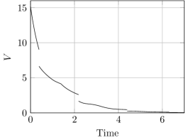
(b) Lyapunov-Krasovskii functional.

Figure 1: Trajectory and value of the Lyapunov-Krasovskii functional in the Example 4.1.

4.2 Reset system with a nonlinear and time varying base system

In general, for a reset system with nonlinear and time-varying base system without a particular structure, there is not systematic procedure for generating Lyapunov-Krasovskii functionals candidates. Therefore, in this section the main result is applied to a reset system with a particular structure.

Example 4.2: Consider a second-order reset system given by

$$\left\{\begin{array}[]{ll}\left\{\begin{array}[]{l}\dot{x}_{1}(t)=a_{1}(t)x_{1}^{3}(t)+b_{1}(t)x_{1}^{3}(t-h)+c_{1}(t)x_{2}(t)\\ \dot{x}_{2}(t)=a_{2}(t)x_{2}(t)+b_{2}(t)x_{2}(t-h)+c_{2}(t)x_{1}^{3}(t)\end{array}\right\},&{\color[rgb]{0,0,0}(x_{1}(t),x_{2}(t))\neq 0,}\\ \\ \left\{\begin{array}[]{l}x_{1}(t^{+})=x_{1}(t)\\ x_{2}(t^{+})=0\end{array}\right\},&{\color[rgb]{0,0,0}(x_{1}(t),x_{2}(t))=0.}\end{array}\right.$$ (31)

where $a_{1}(t)$, $b_{1}(t)$, $c_{1}(t)$, $a_{2}(t)$, $b_{2}(t)$, and $c_{2}(t)$ are arbitrary continuous bounded functions with $a_{1}(t),a_{2}(t)\leq-\delta$, $|b_{1}(t)|,|b_{2}(t)|\leq\frac{\delta}{2}$, and $|c_{1}(t)|,|c_{2}(t)|\leq\frac{\delta}{4}$ for some given $\delta>0$. Here, the reset set $\mathcal{M}$ is given as $\mathcal{M}=\{(x_{1},x_{2})\in\mathds{R}^{2}:\mathbf{g}(x_{1},x_{2})=0,\text{for some }\mathbf{g}:\mathds{R}^{2}\rightarrow\mathds{R}\}$.

Consider the candidate functional $V$ be defined by

$$V({\bf x}_{t})=\frac{x_{1}^{4}(t)}{4}+\frac{x_{2}^{2}(t)}{2}+\frac{\delta}{2}\int^{0}_{-h}\left(x_{1}^{6}(t+\alpha)+x_{2}^{2}(t+\alpha)\right)d\alpha,$$ (32)

where ${\bf x}(t)=(x_{1}(t),x_{2}(t))\in\mathds{R}^{2}$ and ${\bf x}_{t}=x(t+\alpha)$, $\alpha\in[-h,0]$. Let define the continuous nondecreasing functions $u(s)=\frac{1}{4}s^{4}$ and $v(s)=2s^{2}$, then the above functional satisfies condition (6),

$$u(\|{\bf x}_{t}(0)\|)=\frac{1}{4}(x_{1}^{2}(t)+x_{2}^{2}(t))^{2}\leq\frac{1}{4}(x_{1}^{4}(t)+x_{2}^{2}(t))\leq V({\bf x}_{t})$$ (33)

and

$$V({\bf x}_{t})\leq x_{1}^{2}(t)+x_{2}^{2}(t)+\frac{\delta}{2}\int^{0}_{-h}\left(x_{1}^{2}(t+\alpha)+x_{2}^{2}(t+\alpha)\right)d\alpha\leq 2\|{\bf x}_{t}\|^{2}.$$ (34)

It is easy to check that the above conditions are satisfied for any $\|{\bf x}_{t}\|\leq\gamma=\sqrt{\frac{1}{5}}$.

On the other hand, the derivative of the functional along the solutions of system (31) is given by

$$\dot{V}({\bf x}_{t})=x_{1}^{3}(t)\dot{x}_{1}(t)+x_{2}(t)\dot{x}_{2}(t)+\frac{\delta}{2}(x_{1}^{6}(t)-x_{1}^{6}(t-h))+\frac{\delta}{2}(x_{2}^{2}(t)-x_{2}^{2}(t-h)).$$ (35)

After some manipulations the derivative of the functional is bounded by

$$\dot{V}({\bf x}_{t})\leq\xi^{\top}(t)M\xi(t),$$ (36)

where $\xi(t)=\left(|x_{1}(t)|^{3},|x_{1}(t-h)|^{3},|x_{2}(t)|,|x_{2}(t-h)|\right)$ and

$$M=\left(\begin{array}[]{rrrr}-\frac{\delta}{2}&\frac{\delta}{4}&\frac{\delta}{4}&0\\ \frac{\delta}{4}&-\frac{\delta}{2}&0&0\\ \frac{\delta}{4}&0&-\frac{\delta}{2}&\frac{\delta}{4}\\ 0&0&\frac{\delta}{4}&-\frac{\delta}{2}\\ \end{array}\right).$$ (37)

Since $M<0$ for any $\delta>0$, then defining $w(s)=\lambda_{m}(-M)s^{6}$ it follows

$$-\dot{V}({\bf x}_{t})\geq\lambda_{m}(-M)\left(|x_{1}(t)|^{6}+|x_{1}(t-h)|^{6}+|x_{2}(t)|^{2}\right.\left.+|x_{2}(t-h)|^{2}\right)\geq w(\|{\bf x}(t)\|)$$ (38)

for any $\|{\bf x}_{t}\|\leq\sqrt{\frac{1}{5}}$, and thus condition (7) is satisfied. Finally, $\Delta V({\bf x}_{t})=-\frac{x^{2}_{2}(t)}{2}$, which is negative for any reset instant, regardless of the function ${\bf g}$. Hence, the solution ${\bf x}_{t}=0$ of the system (31) is uniformly asymptotically stable.

Now, consider the reset system with functions $a_{1}(t)$, $b_{1}(t)$, $c_{1}(t)$, $a_{2}(t)$, $b_{2}(t)$, and $c_{2}(t)$ given by

$$\begin{array}[]{lllll}a_{1}(t)=50e^{-t}-100\delta,&&b_{1}(t)=\frac{\delta}{2}\sin(t),&&c_{1}(t)=\frac{\delta}{4},\\ a_{2}(t)=-e^{-t}-\delta,&&b_{2}(t)=-\frac{\delta}{2},&&c_{2}(t)=\frac{\delta}{4}\sin(t).\end{array}$$ (39)

It can be easily seen that the above functions satisfy the required bounds for any $\delta>0.51$. In addition, consider the function ${\bf g}(x_{1},x_{2})=-5x_{1}+x_{2}$ and the initial condition $\phi(t)=(\frac{1}{2\sqrt{5}},-\frac{1}{2\sqrt{5}})$, $t\in[t_{0}-h,0]$ such that $\|\phi\|=\frac{1}{\sqrt{10}}<\frac{1}{\sqrt{5}}$. The evolution of the system with $h=1$ and $t_{0}=0$ is plotted in Fig. 2. In addition, Fig. 2 shows the value of the functional (32) along the trajectory. Once again, it can be observed how the functional always decreases.

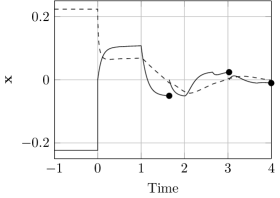
(a) Trajectory: $x_{1}$ (dashed) and $x_{2}$ (solid).

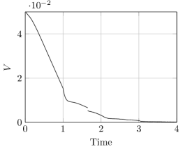
(b) Lyapunov-Krasovskii functional.

Figure 2: Trajectory and value of the Lyapunov-Krasovskii functional in the Example 4.2.

5 Conclusions

This work provides Lyapunov-Krasovskii based conditions that guarantee the stability of time-delay reset systems. In comparison with previous works, the main contribution has been to consider reset systems, whose base system is nonlinear and time-varying. As an application, the proposed result have been applied to obtain delay-independent condition in terms of LMI for time-delay reset control systems. In addition, the stability of a particular reset system with nonlinear and time-varying base system is analyzed.

References

References

• [1] J. C. Clegg, A nonlinear integrator for servomechanisms, Trans. of the American Institute of Electrical Engineering 77 (1958) 41–42.
• [2] K. R. Krishman, I. M. Horowitz, Synthesis of a non-linear feedback system with significant plant-ignorance for prescribed system tolerances, International Journal of Control 19 (4) (1974) 689–706.
• [3] I. M. Horowitz, P. Rosenbaum, Non-linear design for cost of feedback reduction in systems with large parameter uncertainty, International Journal of Control 21 (6) (1975) 977–1001.
• [4] A. Baños, A. Barreiro, Reset Control Systems, Advances in Industrial Control, Springer, 2012.
• [5] K. J. Åström, Limitations on control system performance, European Journal of Control 6 (2000) 2–20.
• [6] O. Beker, C. Hollot, Y. Chait, Plant with integrator: an example of reset control overcoming limitations of linear feedback, IEEE Transaction on Automatic Control 46 (11) (2001) 1797–1799.
• [7] M. A. Davó, A. Baños, Reset control of a liquid level process, in: IEEE 18th Conference on Emerging Technologies & Factory Autom., IEEE, 2013, pp. 1–4.
• [8] J. Moreno, J. Guzmán, J. Normey-Rico, A. Baños, M. Berenguel, A combined FSP and reset control approach to improve the set-point tracking task of dead-time processes, Control Engineering Practice 21 (4) (2013) 351–359.
• [9] O. Beker, C. V. Hollot, Y. Chait, H. Han, Fundamental properties of reset control systems, Automatica 40 (6) (2004) 905–915.
• [10] J. K. Hale, S. M. V. Lunel, Introduction to functional differential equations, Springer, New York, 1993.
• [11] K. Gu, J. Chen, V. Kharitonov, Stability of Time-Delay Systems, Birkhäuser, 2003.
• [12] E. Fridman, Introduction to Time-Delay Systems, Systems & Control: Foundations & Applications, Birkhäuser, 2014.
• [13] E. Fridman, A descriptor system approach to ${H}_{\infty}$ control of linear time-delay systems, IEEE Transaction on Automatic Control 47 (2) (2002) 253–270.
• [14] J. Cao, J. Wang, Delay-dependent robust stability of uncertain nonlinear systems with time-delay, Applied Mathematics and Computation 154 (1) (2004) 289–297.
• [15] F. Ren, J. Cao, Novel $\alpha$-stability criterion of linear systems with multiple time delays, Applied Mathematics and Computation 181 (1) (2006) 282–290.
• [16] F. Gouaisbaut, D. Peaucelle, Delay-dependent stability of time-delay systems, in: Proceedings of the 5th IFAC Symposium on Robust Control Design, Toulouse, France, 2006, pp. 453–458.
• [17] A. Seuret, F. Gouaisbaut, Wirtinger-base integral inequality: application to time-delay systems, Automatica 49 (9) (2013) 2860–2866.
• [18] A. Baños, A. Barreiro, Delay-independent stability of reset control systems, IEEE Transaction on Automatic Control 54 (2009) 341–346.
• [19] A. Barreiro, A. Baños, Delay-dependent stability of reset systems, Automatica 46 (2010) 216–221.
• [20] D. D. Bainov, P. S. Simeonov, Systems with Impulse Effect: Stability, Theory and Applications, Ellis Horwood, Chichester, UK, 1989.
• [21] V. Lakshmikantham, D. D. Bainov, P. S. Simeonov, Theory of Impulsive Differential Equations, World Scientific, Singapore, 1989.
• [22] W. M. Haddad, V. S. Chellaboina, S. G. Nersesov, Impulsive and Hybrid Dynamical Systems: Stability, Dissipativity, and Control, Princeton Series in Applied Mathematics, 2006.
• [23] A. N. Michel, L. Hou, D. Liu, Stability of dynamical systems: continuous, discontinuous, and discrete systems, Birkhauser, Boston, 2007.
• [24] A. Baños, J. I. Mulero, Well-posedness of reset control systems as state-dependent impulsive dynamical sysetms, Abstract and Applied Analysis 2012.
• [25] G. Ballinger, X. Liu, Existence, uniqueness and boundedness results for impulsive delay differential equations, Applicable Analysis: An international Journal 74 (1-2) (2000) 71–93.
• [26] M. de la Sen, N. Luo, A note on the stability of linear time-delay systems with impulsive inputs, IEEE Transactions on Circuits and Systems I: Fundamental Theory and Applications 50 (1) (2003) 149–152.
• [27] X. Liu, Stability of impulsive control systems with time delay, Mathematical and Computer Modelling 39 (2004) 511–519.
• [28] X. Liu, X. Shen, Y. Zhang, Q. Wang, Stability criteria for impulsive systems with time delay and unstable system matrices, IEEE Transaction on circuits and systems 54 (10) (2007) 2288–2298.
• [29] P. Haghshtabrizi, J. P. Hespanha, A. R. Teel, Stability of delay impulsive systems with application to networked control systems, Transaction of the Institute of measurement and control 32 (5) (2009) 511–528.
• [30] Y. Sun, A. N. Michel, G. Zhai, Stability of discontinuous retarded functional differential equations with applications, IEEE Transactions on Automatic Control 50 (8) (2005) 1090–1105.
• [31] X. Liu, Q. Wang, The method of lyapunov functionals and exponential stability of impulsive systems with time delay, Nonlinear Analysis 66 (2007) 1465–1454.
• [32] I. M. Stamova, Stability Analysis of Impulsive Functional Differential Equations, Walter de Gruyter, 2009.
• [33] J. A. Prieto, A. Barreiro, S. Dormido, S. Tarbouriech, Delay-dependent stability of reset control systems with anticipative reset conditions, in: IFAC Symposium on Robust Control Design, 2012, pp. 219–224.
• [34] Y. Guo, L. Xie, Quadratic stability of reset control systems with delays, in: 10th World Congress on Intelligent Control and Automation (WCICA), 2012, pp. 2268–2273.
• [35] M. A. Davó, A. Baños, Delay-dependent stability of reset control systems with input/output delays, in: IEEE 52nd Annual Conference on Decision and Control (CDC), 2013, pp. 2018–2023.
• [36] P. Mercader, M. A. Davó, A. Baños, $\mathcal{H}_{\infty}$/$\mathcal{H}_{2}$ analysis for time-delay reset control systems, in: 3rd International Conference on Systems and Control (ICSC), 2013, pp. 518–523.
• [37] P. Mercader, J. Carrasco, A. Baños, IQC analysis for time-delay reset control systems with first order reset elements, in: IEEE 52nd Annual Conference on Decision and Control (CDC), 2013, pp. 2251–2256.
• [38] J. Carrasco, A. Baños, A. van der Schaft, A passivity-based approach to reset control systems stability, Systems & Control Letters 59 (1) (2010) 18–24.
• [39] J. Liu, A. Teel, Generalized solutions to hybrid systems with delays, in: Proceedings of the 51st Annual Conference on Decision and Control, 2012, pp. 6169–6174.
• [40] J. Liu, A. Teel, Hybrid systems with memory: Modelling and stability analysis via generalized solutions, in: Proceedings of the 19th IFAC World Congress, 2014.
• [41] A. Baños, F. Perez, S. Tarbouriech, L. Zaccarian, Low-Complexity Controllers for Time-Delay Systems: Delay-independent stability via reset loops, Advances in Delays and Dynamics, Springer International Publishing, 2014, Ch. 8, pp. 111–125.
• [42] R. Goebel, A. R. Teel, R. G. Sanfelice, Hybrid Dynamical Systems: Modeling, Stability, and Robustness, Princeton University Press, 2012.