Quasi Monte Carlo integration and kernel-based function approximation on Grassmannians

Abstract

Numerical integration and function approximation on compact Riemannian manifolds based on eigenfunctions of the Laplace-Beltrami operator have been widely studied in the recent literature. The standard example in numerical experiments is the Euclidean sphere. Here, we derive numerically feasible expressions for the approximation schemes on the Grassmannian manifold, and we present the associated numerical experiments on the Grassmannian. Indeed, our experiments illustrate and match the corresponding theoretical results in the literature.

1 Introduction

The present paper is dedicated to numerical experiments concerning two classical problems in numerical analysis, numerical integration and function approximation. The novelty of our experiments is that we work on the Grassmannian manifold as an example of a compact Riemannian manifold illustrating theoretical results in the recent literature.

Indeed, recent data analysis methodologies involve kernel based approximation of functions on manifolds and other measure spaces, cf. Maggioni:2008fk ; Mhaskar:2010kx and Geller:2011fk ; Geller:2012fk ; Geller:2013uk . The kernels are build up by what is known as diffusion polynomials, which are eigenfunctions of elliptic differential operators, commonly chosen as the Laplace-Beltrami operator when dealing with compact Riemannian manifolds.

Numerical implementations of the approximation schemes require pointwise evaluation of the eigenfunctions. However, explicit formulas for eigenfunctions are only known in few special cases. If the manifold is the unit sphere $\mathbb{S}^{d-1}$, for instance, then the eigenfunctions of the spherical Laplacian are the spherical harmonics, which are indeed polynomials in the usual sense. The corresponding kernels for the sphere have been computed explicitly in Gia:2006fk ; Gia:2008fk .

The kernel based approximation requires the computation of the corresponding integral operator, see (7) in Section 3. In the realm of numerical integration, the integral itself is usually approximated by a weighted sum over sample values, see also Filbir:2010aa ; Filbir:2011fk . The latter fits well to the common scenario when the target function needs to be approximated from a finite sample in the first place.

Numerical integration on Euclidean spaces is a classical problem in numerical analysis. Recently, Quasi Monte Carlo (QMC) numerical integration on compact Riemannian manifolds has been studied in Brandolini:2014oz from a theoretical point of view, see also Pesenson:2012fp . If more and more samples are used, then the smoothness parameter of Bessel potential spaces steers the decay of the integration error. QMC integration has been introduced for the sphere in Brauchart:fk , where many explicit examples are provided and extensive numerical experiments illustrate the theoretical claims.

The major aim of the present paper is to provide numerical experiments for the above integration and approximation schemes when the manifold is the Grassmannian, i.e., the collection of $k$-dimensional subspaces in $\mathbb{R}^{d}$, naturally identified with the collection $\mathcal{G}_{k,d}$ of rank-$k$ orthogonal projectors on $\mathbb{R}^{d}$, cf. (Chikuse:2003aa, , Chapter 1).

Therefore, we require explicit formulas of the kernels used in Maggioni:2008fk ; Mhaskar:2010kx . Indeed, the degree of a diffusion polynomial, by definition, relates to the magnitude of the corresponding eigenvalues. We check that diffusion polynomials of degree at most $2t/\sqrt{k}$ are indeed usual multivariate polynomials of degree $t$ restricted to the Grassmannian. The explicit formula for the kernel is derived through generalized Jacobi polynomials. By computing cubature formulas on Grassmannians through some numerical minimization process, we are able to provide numerical experiments for the approximation of functions on Grassmannians and for the QMC integration on Grassmannians supporting the theoretical results in Brandolini:2014oz ; Maggioni:2008fk ; Mhaskar:2010kx .

The outline is as follows: In Section 2 we recall QMC integration from Brandolini:2014oz ; Brauchart:fk , and we recall the approximation scheme from Maggioni:2008fk ; Mhaskar:2010kx in the special case of the Grassmannian in Section 3. Section 4 provides feasible formulations for numerical experiments. Indeed, Section 4.1 is devoted to derive explicit formulas for the involved kernel by means of generalized Jacobi polynomials. We check the relations between diffusion polynomials and ordinary polynomials restricted to the Grassmannian in Section 4.2, and we provide the framework for numerically computing cubatures in Grassmannians in Section 4.3. The numerical experiments are provided in Section 5.

2 Quasi Monte Carlo integration

We identify the Grassmannian, the collection of $k$-dimensional subspaces in $\mathbb{R}^{d}$, with the set of orthogonal projectors on $\mathbb{R}^{d}$ of rank $k$, denoted by

$$\mathcal{G}_{k,d}:=\{P\in\mathbb{R}^{d\times d}_{\operatorname{sym}}:P^{2}=P;\;\operatorname{tr}(P)=k\}.$$

Here, $\mathbb{R}^{d\times d}_{\operatorname{sym}}$ is the set of symmetric matrices in $\mathbb{R}^{d\times d}$ and $\operatorname{tr}(P)$ denotes the trace of $P$. The dimension of the Grassmannian is $\dim(\mathcal{G}_{k,d})=k(d-k)$. The canonical Riemannian measure on $\mathcal{G}_{k,d}$ is denoted by $\mu_{k,d}$, which we assume to be normalized to one. Without loss of generality, we assume $k\leq\frac{d}{2}$ throughout since $\mathcal{G}_{d-k,d}$ can be identified with $\mathcal{G}_{k,d}$.

As a classical problem in numerical analysis, we aim to approximate the integral over a continuous function $f:\mathcal{G}_{k,d}\rightarrow\mathbb{C}$ by a finite sum over weighted samples, i.e., we consider points $\{P_{j}\}_{j=1}^{n}\subset\mathcal{G}_{k,d}$ and nonnegative weights $\{\omega_{j}\}_{j=1}^{n}$ such that

$$\sum_{j=1}^{n}\omega_{j}f(P_{j})\approx\int_{\mathcal{G}_{k,d}}f(P)\mathrm{d}\mu_{k,d}(P).$$

In order to quantify the error by means of the smoothness of $f$, we shall define Bessel potential spaces on $\mathcal{G}_{k,d}$, for which we need some preparation. Let $\{\varphi_{\ell}\}_{\ell=0}^{\infty}$ be the collection of orthonormal eigenfunctions of the Laplace-Beltrami operator $\Delta$ on $\mathcal{G}_{k,d}$, and $\{-\lambda_{\ell}\}_{\ell=0}^{\infty}$ are the corresponding eigenvalues arranged, so that $0=\lambda_{0}\leq\lambda_{1}\leq\ldots$. Without loss of generality, we choose each $\varphi_{\ell}$ to be real-valued, in particular, $\varphi_{0}\equiv 1$. The Fourier transform of $f\in L_{p}(\mathcal{G}_{k,d})$, where $1\leq p\leq\infty$, is defined by

$$\hat{f}(\ell):=\int_{\mathcal{G}_{k,d}}f(P)\varphi_{\ell}(P)\mathrm{d}\mu_{k,d}(P),\qquad\ell=0,1,2,\ldots.$$

Essentially following Brandolini:2014oz ; Mhaskar:2010kx , we formally define $(I-\Delta)^{s/2}f$ to be the distribution on $\mathcal{G}_{k,d}$, such that $\langle(I-\Delta)^{s/2}f,\varphi_{\ell}\rangle=(1+\lambda_{\ell})^{s/2}\langle f,\varphi_{\ell}\rangle$, for all $\ell=0,1,2,\ldots$. The Bessel potential space $H^{s}_{p}(\mathcal{G}_{k,d})$, for $1\leq p\leq\infty$ and $s\geq 0$, is

$$H^{s}_{p}(\mathcal{G}_{k,d}) :=\{f\in L_{p}(\mathcal{G}_{k,d}):\|f\|_{H^{s}_{p}}<\infty\},\quad\text{where}$$

$$\|f\|_{H^{s}_{p}} :=\|(I-\Delta)^{s/2}f\|_{L_{p}},$$

i.e., $f\in H^{s}_{p}(\mathcal{G}_{k,d})$ if and only if $f\in L_{p}(\mathcal{G}_{k,d})$ and $(I-\Delta)^{s}f\in L_{p}(\mathcal{G}_{k,d})$. Note that this definition is indeed consistent with Brandolini:2014oz ; Mhaskar:2010kx , see (Brandolini:2014oz, , Theorem 2.1, Definition 2.2) in particular. For $s>k(d-k)/p$ with $1\leq p\leq\infty$, the space $H^{s}_{p}(\mathcal{G}_{k,d})$ is embedded into the space of continuous functions on $\mathcal{G}_{k,d}$, see, for instance, Brandolini:2014oz . For $1<p<\infty$, this embedding also follows from results on Bessel potential spaces on general Riemannian manifolds with bounded geometry, cf. (Triebel:1992aa, , Theorem 7.4.5, Section 7.4.2), and on $\mathbb{R}^{d}$ with $1\leq p\leq\infty$, see (Stein:1970yg, , Chapter V, 6.11). According to Brandolini:2014oz , for any sequence of points $\{P^{t}_{j}\}_{j=1}^{n_{t}}\subset\mathcal{G}_{k,d}$, $t=0,1,2,\ldots$, and positive weights $\{\omega^{t}_{j}\}_{j=1}^{n_{t}}\subset\mathbb{R}$ with $n_{t}\rightarrow\infty$, there is a function $f\in H^{s}_{p}(\mathcal{G}_{k,d})$ such that

$$\Big{|}\int_{\mathcal{G}_{k,d}}f(P)\mathrm{d}\mu_{k,d}(P)-\sum_{j=1}^{n_{t}}\omega^{t}_{j}f(P^{t}_{j})\Big{|}\gtrsim n_{t}^{-\frac{s}{k(d-k)}}\|f\|_{H^{s}_{p}},$$ (1)

where the constant does not depend on $t$. Thus, we cannot do any better than the rate

$$n_{t}^{-\frac{s}{k(d-k)}}.$$

In order to quantify the quality of weighted point sequences $\{(P^{t}_{j},\omega^{t}_{j})\}_{j=1}^{n_{t}}$, $t=0,1,2,\dots$, for numerical integration, we make the following definition, whose analogous formulation on the sphere (with constant weights) is due to Brauchart:fk .

Definition 1

Given $s>k(d-k)/p$, a sequence $\{(P^{t}_{j},\omega^{t}_{j})\}_{j=1}^{n_{t}}$, $t=0,1,2,\ldots$, of $n_{t}$ points in $\mathcal{G}_{k,d}$ and positive weights with $n_{t}\rightarrow\infty$ is called a sequence of Quasi Monte Carlo (QMC) systems for $H^{s}_{p}(\mathcal{G}_{k,d})$ if

$$\Big{|}\int_{\mathcal{G}_{k,d}}f(P)\mathrm{d}\mu_{k,d}(P)-\sum_{j=1}^{n_{t}}\omega^{t}_{j}f(P^{t}_{j})\Big{|}\lesssim n_{t}^{-\frac{s}{k(d-k)}}\|f\|_{H^{s}_{p}}$$

holds for all $f\in H^{s}_{p}(\mathcal{G}_{k,d})$.

In case $p=2$, given $s>k(d-k)/2$, any sequence of QMC systems $\{(P^{t}_{j},\omega^{t}_{j})\}_{j=1}^{n_{t}}$ for $H^{s}_{2}(\mathcal{G}_{k,d})$ is also a sequence of QMC systems for $W^{s^{\prime}}_{2}(\mathcal{G}_{k,d})$, for all $s^{\prime}$ satisfying $s\geq s^{\prime}>k(d-k)/2$, cf. Brandolini:2014oz .

Especially for the integration of smooth functions, random points lack quality when compared to QMC systems.

Proposition 1

For $s>k(d-k)/2$, suppose $P_{1},\ldots,P_{n}$ are random points on $\mathcal{G}_{k,d}$, independently identically distributed according to $\mu_{k,d}$ then it holds

$$\sqrt{\mathbb{E}\Big{[}\sup_{\begin{subarray}{c}f\in H^{s}_{2}(\mathcal{G}_{k,d})\\ \|f\|_{H^{s}_{2}}\leq 1\end{subarray}}\Big{|}\int_{\mathcal{G}_{k,d}}f(P)\mathrm{d}\mu_{k,d}(P)-\frac{1}{n}\sum_{j=1}^{n}f(P_{j})\Big{|}^{2}\Big{]}}=cn^{-\frac{1}{2}}$$

with $c^{2}=\sum_{\ell=1}^{\infty}(1+\lambda_{\ell})^{-s}$.

Note that the condition $s>k(d-k)/2$ implies that $\frac{s}{k(d-k)}>\frac{1}{2}$, so that on average QMC systems indeed perform better than random points for smooth functions. The proof of Proposition 1 is derived by following the lines in Brauchart:fk . In fact, the result is already contained in (Graf:2013zl, , Corollary 2.8), see also Nowak:2010rr , within a more general setting.

In order to derive QMC systems, we shall have a closer look at cubature points, for which we need the space of diffusion polynomials of degree at most $t$, defined by

$$\Pi_{t}:=\operatorname*{span}\{\varphi_{\ell}:\lambda_{\ell}\leq t^{2}\},$$ (2)

see Mhaskar:2010kx and references therein.

Definition 2

For $\{P_{j}\}_{j=1}^{n}\subset\mathcal{G}_{k,d}$ and positive weights $\{\omega_{j}\}_{j=1}^{n}$, we say that $\{(P_{j},\omega_{j})\}_{j=1}^{n}$ is a cubature for $\Pi_{t}$ if

$$\int_{\mathcal{G}_{k,d}}f(P)\mathrm{d}\mu_{k,d}(P)=\sum_{j=1}^{n}\omega_{j}f(P_{j}),\quad\text{for all }f\in\Pi_{t}.$$ (3)

The number $t$ refers to the strength of the cubature.

In the following result, cf. (Brandolini:2014oz, , Theorem 2.12), the cubature error is bounded by the cubature strength $t$, not the number of points.

Theorem 2.1

Suppose $s>k(d-k)/p$ and assume that $\{(P^{t}_{j},\omega^{t}_{j})\}_{j=1}^{n_{t}}$ is a cubature for $\Pi_{t}$. Then we have, for $f\in H^{s}_{p}(\mathcal{G}_{k,d})$,

$$\Big{|}\int_{\mathcal{G}_{k,d}}f(P)\mathrm{d}\mu_{k,d}(P)-\sum_{j=1}^{n_{t}}\omega^{t}_{j}f(P^{t}_{j})\Big{|}\lesssim t^{-s}\|f\|_{H^{s}_{p}}.$$

Weyl’s estimates on the spectrum of an elliptic operator yield

$$\dim(\Pi_{t})\asymp t^{k(d-k)},$$

cf. (Hormander:1983gf, , Theorem 17.5.3). This implies that any sequence of cubatures $\{(P^{t}_{j},\omega^{t}_{j})\}_{j=1}^{n_{t}}$ of strength $t$, respectively, must obey $n_{t}\gtrsim t^{k(d-k)}$ asymptotically in $t$, cf. Harpe:2005fk . There are indeed sequences of cubatures $\{(P^{t}_{j},\omega^{t}_{j})\}_{j=1}^{n_{t}}$ of strength $t$, respectively, satisfying

$$n_{t}\asymp t^{k(d-k)},$$ (4)

cf. Harpe:2005fk . In this case, Theorem 2.1 leads to

$$\Big{|}\int_{\mathcal{G}_{k,d}}f(P)\mathrm{d}\mu_{k,d}(P)-\sum_{j=1}^{n_{t}}\omega^{t}_{j}f(P^{t}_{j})\Big{|}\lesssim n_{t}^{-\frac{s}{k(d-k)}}\|f\|_{H^{s}_{p}},$$ (5)

so that we have settled that QMC systems do exist, for any $s>k(d-k)/p$, and can be derived via cubatures.

Remark 1

Cubature points $\{P_{j}\}_{j=1}^{n}$ for $\Pi_{t}$ with constant weights $\omega_{j}=\frac{1}{n}$ are called $t$-designs. For all $t=1,2,\ldots$, there exist $t$-designs, cf. Seymour:1984bh . The results in Bondarenko:2011kx imply that there are $t$-designs satisfying (4) provided that $k=1$. However, for $2\leq k\leq\frac{d}{2}$, it is still an open problem if the asymptotics (4) can be achieved by $t$-designs in place of cubatures.

3 Approximation by diffusion kernels

One example, where integrals over the Grassmannian are replaced with weighted finite sums, is the approximation of a function $f:\mathcal{G}_{k,d}\rightarrow\mathbb{C}$ from finitely many samples. The approximation scheme developed in Maggioni:2008fk ; Mhaskar:2010kx works for manifolds and metric measure spaces in general, but we shall restrict the presentation to the Grassmannian.

For a function $f\in L_{p}(\mathcal{G}_{k,d})$, we denote the (polynomial) best approximation error by

$$\operatorname{dist}(f,\Pi_{t})_{L_{p}}:=\inf_{g\in\Pi_{t}}\|f-g\|_{L_{p}},$$

where $t\geq 0$. It is possible to quantify the best approximation error in dependence of the function’s smoothness, see (Mhaskar:2010kx, , Proposition 5.3) for the following result.

Theorem 3.1

If $f\in H^{s}_{p}(\mathcal{G}_{k,d})$, then

$$\operatorname{dist}(f,\Pi_{t})_{L_{p}}\lesssim t^{-s}\|f\|_{H^{s}_{p}}.$$

Given $f\in H^{s}_{p}(\mathcal{G}_{k,d})$ we now construct a particular sequence of functions $\sigma_{t}(f)\in\Pi_{t}$, $t=1,2,\ldots$, that realizes this best approximation rate. Note that, since the collection $\{\varphi_{\ell}\}_{\ell=0}^{\infty}$ is an orthonormal basis for $L_{2}(\mathcal{G}_{k,d})$, any function $f\in L_{2}(\mathcal{G}_{k,d})$ can be expanded as a Fourier series by

$$f=\sum_{\ell=0}^{\infty}\hat{f}(\ell)\varphi_{\ell}.$$

The approach in Maggioni:2008fk ; Mhaskar:2010kx makes use of a smoothly truncated Fourier expansion of $f$,

$$\sigma_{t}(f):=\sum_{\ell=0}^{\infty}h(t^{-2}\lambda_{\ell})\hat{f}(\ell)\varphi_{\ell}\in\Pi_{t},$$

where $h:\mathbb{R}_{\geq 0}\rightarrow\mathbb{R}$ is an infinitely often differentiable and nonincreasing function with $h(x)=1$, for $x\leq 1/2$, and $h(x)=0$, for $x\geq 1$. Using the kernel $K_{t}$ on $\mathcal{G}_{k,d}\times\mathcal{G}_{k,d}$ defined by

$$K_{t}(P,Q)=\sum_{\ell=0}^{\infty}h(t^{-2}\lambda_{\ell})\varphi_{\ell}(P)\varphi_{\ell}(Q)$$ (6)

we arrive after interchanging summation and integration at the following alternative representation

$$\sigma_{t}(f)=\int_{\mathcal{G}_{k,d}}f(P)K_{t}(P,\cdot)\mathrm{d}\mu_{k,d}(P).$$ (7)

Note, that the function $\sigma_{t}(f)$ is well-defined for general $f\in L_{p}(\mathcal{G}_{k,d})$, $1\leq p\leq\infty$, and it turns out that $\sigma_{t}(f)$ approximates $f$ up to a constant as good as the best approximation from $\Pi_{t}$, cf. (Mhaskar:2010kx, , Proposition 5.3).

Theorem 3.2

If $f\in H^{s}_{p}(\mathcal{G}_{k,d})$, then

$$\|f-\sigma_{t}(f)\|_{L_{p}}\lesssim t^{-s}\|f\|_{H^{s}_{p}}.$$

If $f$ needs to be approximated from a finite sample, then $\sigma_{t}(f)$ in (7) cannot be determined directly and is replaced with a weighted finite sum in Mhaskar:2010kx . Indeed, for sample points $\{P_{j}\}_{j=1}^{n}\subset\mathcal{G}_{k,d}$ and weights $\{\omega_{j}\}_{j=1}^{n}$, we define

$$\sigma_{t}(f,\{(P_{j},\omega_{j})\}_{j=1}^{n}):=\sum_{j=1}^{n}\omega_{j}f(P_{j})K_{t}(P_{j},\cdot).$$ (8)

Note that we must now consider functions $f$ in Bessel potential spaces, for which point evaluation makes sense. We shall observe in the following that if samples and weights satisfy some cubature type property, then the approximation rate is still preserved when using $\sigma_{t}(f,\{(P_{j},\omega_{j})\}_{j=1}^{n})$ in place of $\sigma_{t}(f)$. However, we need an additional technical assumption on the points $\{P_{j}\}_{j=1}^{n}$, for which we denote the geodesic distance between $P,Q\in\mathcal{G}_{k,d}$ by

$$\rho(P,Q)=\sqrt{\theta_{1}^{2}+\ldots+\theta_{k}^{2}},$$

where $\theta_{1},\ldots\theta_{k}$ are the principal angles between the associated subspaces of $P$ and $Q$ respectively, i.e.,

$$\theta_{i}=\arccos(\sqrt{y_{i}}),\quad i=1,\ldots,k,$$

and $y_{1},\ldots,y_{k}$ are the $k$ largest eigenvalues of the matrix $PQ$. We define the ball of radius $r$ centered around $P\in\mathcal{G}_{k,d}$ by

$$\mathbb{B}_{r}(P):=\{Q\in\mathcal{G}_{k,d}:\rho(P,Q)\leq r\}.$$

The following approximation from finitely many sample points is due to (Mhaskar:2010kx, , Proposition 5.3).

Theorem 3.3

For $t=1,2,\ldots$, suppose we are given a sequence of point sets $\{P^{t}_{j}\}_{j=1}^{n_{t}}\subset\mathcal{G}_{k,d}$ and positive weights $\{\omega_{j}^{t}\}_{j=1}^{n_{t}}$ such that

$$\int_{\mathcal{G}_{k,d}}g_{1}(P)g_{2}(P)\mathrm{d}\mu_{k,d}(P)=\sum_{j=1}^{n_{t}}\omega_{j}^{t}g_{1}(P^{t}_{j})g_{2}(P^{t}_{j}),\qquad g_{1},g_{2}\in\Pi_{t}.$$ (9)

Then the approximation error, for $f\in H^{s}_{\infty}(\mathcal{G}_{k,d})$, is bounded by

$$\|f-\sigma_{t}(f,\{(P^{t}_{j},\omega^{t}_{j})\}_{j=1}^{n_{t}})\|_{L_{\infty}}\lesssim t^{-s}(\|f\|_{L_{\infty}}+\|f\|_{H^{s}_{\infty}}).$$ (10)

Note that the original result stated in Mhaskar:2010kx requires an additional regularity condition on the samples. This condition is satisfied since we restrict us to positive weights, cf. (Filbir:2011fk, , Theorem 5.5 (a)). The assumption (9) is a cubature type condition, for which our results in Section 4.2 shall provide further clarification. It indeed turns out that there are sequences $\{(P^{t}_{j},\omega^{t}_{j})\}_{j=1}^{n_{t}}$ satisfying (9) with $n_{t}\asymp t^{k(d-k)}$, in which case (10) becomes

$$\|f-\sigma_{t}(f,\{(P^{t}_{j},\omega^{t}_{j})\}_{j=1}^{n_{t}})\|_{L_{\infty}}\lesssim n_{t}^{-\frac{s}{k(d-k)}}(\|f\|_{L_{\infty}}+\|f\|_{H^{s}(L_{\infty})}).$$ (11)

Note that the approximation rate in (11) matches the one in (5) for the integration error. The proof of Theorem 3.3 in Mhaskar:2010kx is indeed based on Theorem 3.2 and on the approximation of the integral $\sigma_{t}(f)$ in (7) by the weighted finite sum $\sigma_{t}(f,\{(P^{t}_{j},\omega_{j}^{t})\}_{j=1}^{n})$ in (8). For related results on local smoothness and approximation, we refer to Ehler:2012fk .

4 Numerically feasible formulations

This section is dedicated to turn the approximation schemes presented in the previous sections into numerically feasible expressions. In other words, we determine explicit expressions for the kernel $K_{t}$ in (6) and provide an optimization method for the numerical computation of cubature points or QMC systems on the Grassmannian.

4.1 Diffusion kernels on Grassmannians

The probability measure $\mu_{k,d}$ is invariant under orthogonal conjugation and induced by the Haar (probability) measure $\mu_{\mathcal{O}(d)}$ on the orthogonal group $\mathcal{O}(d)$, i.e., for any $Q\in\mathcal{G}_{k,d}$ and measurable function $f$, we have

$$\int_{\mathcal{G}_{k,d}}f(P)\mathrm{d}\mu_{k,d}(P)=\int_{\mathcal{O}(d)}f(OQO^{\top})\mathrm{d}\mu_{\mathcal{O}(d)}(O).$$

By the orthogonal invariance of the Laplace-Beltrami operator $\Delta$ on $\mathcal{G}_{k,d}$ it is convenient for the description of the eigenfunctions to recall the irreducible decomposition of $L_{2}(\mathcal{G}_{k,d})$ with respect to the orthogonal group. Given a nonnegative integer $t$, a partition of $t$ is an integer vector $\pi=(\pi_{1},\dots,\pi_{t})$ with $\pi_{1}\geq\ldots\geq\pi_{t}\geq 0$ and $|\pi|=t$, where $|\pi|:=\sum_{i=1}^{t}\pi_{i}$ is the size of $\pi$. The length $l(\pi)$ is the number of nonzero parts of $\pi$. The space $L_{2}(\mathcal{G}_{k,d})$ decomposes into

$$L_{2}(\mathcal{G}_{k,d})=\bigoplus_{l(\pi)\leq k}H_{\pi}(\mathcal{G}_{k,d}),\qquad H_{\pi}(\mathcal{G}_{k,d})\perp H_{\pi^{\prime}}(\mathcal{G}_{k,d}),\quad\pi\neq\pi^{\prime},$$ (12)

where $H_{\pi}(\mathcal{G}_{k,d})$ is equivalent to $\mathcal{H}_{2\pi}^{d}$, the irreducible representation of $\mathcal{O}(d)$ associated to the partition $2\pi=(2\pi_{1},\dots,2\pi_{t})$, cf. Bachoc:2002aa ; James:1974aa .

By orthogonal invariance the spaces $H_{\pi}(\mathcal{G}_{k,d})$ are eigenspaces of the Laplace-Beltrami operator $\Delta$ on $\mathcal{G}_{k,d}$ where, according to (James:1974aa, , Theorem 13.2), the associated eigenvalues are

$$\lambda(\pi)=2|\pi|d+4\sum_{i=1}^{k}\pi_{i}(\pi_{i}-i).$$ (13)

Note, for a given eigenvalue $\lambda_{\ell}$ the corresponding eigenspace can decompose into more than one irreducible subspace $H_{\pi}(\mathcal{G}_{k,d})$.

Note that the following results are translations from representation theory used in James:1974aa , see also Bachoc:2002aa ; Bachoc:2006aa , into the terminology of reproducing kernels, where we have only adapted the scaling of the kernels. The space $H_{\pi}(\mathcal{G}_{k,d})$ equipped with the $L_{2}$ inner product is a finite dimensional reproducing kernel Hilbert space, and its reproducing kernel $K_{\pi}$ is given by

$$K_{\pi}(P,Q)=\sum_{\varphi_{\ell}\in H_{\pi}(\mathcal{G}_{k,d})}\varphi_{\ell}(P)\varphi_{\ell}(Q).$$ (14)

Moreover, $K_{\pi}$ is zonal, i.e., the value $K_{\pi}(P,Q)$ only depends on the $k$ largest eigenvalues

$$y_{1}(P,Q),\ldots,y_{k}(P,Q),$$

of the matrix $PQ$ counted with multiplicities, see James:1974aa . It follows that the kernel $K_{t}$ in (6) is also zonal since it can be written as

$$K_{t}(P,Q)=\sum_{l(\pi)\leq k}h(t^{-2}\lambda(\pi))K_{\pi}(P,Q).$$ (15)

According to James:1974aa , the kernels $K_{\pi}$ are in one-to-one correspondence with generalized Jacobi polynomials. For parameters $\alpha,\beta\in\mathbb{R}$ satisfying $\tfrac{1}{2}(m-1)<\alpha<\beta-\tfrac{1}{2}(m-1)$, the generalized Jacobi polynomials, $J^{\alpha,\beta}_{\pi}:[0,1]^{m}\to\mathbb{R}$ with $l(\pi)\leq m$, are symmetric polynomials of degree $|\pi|$ and form a complete orthogonal system with respect to the density

$$w_{\alpha,\beta}(y_{1},\dots,y_{m}):=\prod_{i=1}^{m}\big{(}y_{i}^{\alpha-\frac{1}{2}(m+1)}(1-y_{i})^{\beta-\alpha-\frac{1}{2}(m+1)}\big{)}\prod_{j=i+1}^{m}|y_{i}-y_{j}|,$$ (16)

where $0<y_{1},\ldots y_{m}<1$, cf. Davis:1999zg ; Dumitriu:2007ax . For the special parameters $\alpha=\tfrac{k}{2}$ with $k\leq\tfrac{d}{2}$ and $\beta=\tfrac{d}{2}$, and the normalization $J_{\pi}^{\frac{k}{2},\frac{d}{2}}(1,\dots,1)=\dim(H_{\pi}(\mathcal{G}_{k,d}))$ the generalized Jacobi polynomials in $m=k$ variables can be identified with the reproducing kernels $K_{\pi}$ of $H_{\pi}(\mathcal{G}_{k,d})$, i.e.,

$$K_{\pi}(P,Q)=J_{\pi}^{\frac{k}{2},\frac{d}{2}}(y_{1}(PQ),\dots,y_{k}(PQ)),\qquad P,Q\in\mathcal{G}_{k,d}.$$ (17)

Now, (15) and (17) yield that the expression for the kernel $K_{t}$ in (6) can be computed explicitly by

$$K_{t}(P,Q) =\sum_{l(\pi)\leq k}h(t^{-2}\lambda(\pi))J_{\pi}^{\frac{k}{2},\frac{d}{2}}(y_{1}(PQ),\dots,y_{k}(PQ)).$$

Thus, avoiding the actual computation of $\{\varphi_{\ell}\}_{\ell=0}^{\infty}$, we have derived the expression of $K_{t}$ by means of generalized Jacobi polynomials.

4.2 Diffusion polynomials on Grassmannians

This section is dedicated to investigate on the relations between diffusion polynomials $\Pi_{t}$ and multivariate polynomials of degree $t$ restricted to the Grassmannian. Indeed, the space of polynomials on $\mathcal{G}_{k,d}$ of degree at most $t$ is defined as restrictions of polynomials by

$$\operatorname{Pol}_{t}(\mathcal{G}_{k,d}):=\{f|_{\mathcal{G}_{k,d}}:f\in\mathbb{C}[X]_{t}\},$$ (18)

where $\mathbb{C}[X]_{t}$ is the collection of multivariate polynomials of degree at most $t$ with $d^{2}$ many variables arranged as a matrix $X\in\mathbb{C}^{d\times d}$. Here, $f|_{\mathcal{G}_{k,d}}$ denotes the restriction of $f$ to $\mathcal{G}_{k,d}$. It turns out that $\operatorname{Pol}_{t}(\mathcal{G}_{k,d})$ is a direct sum of eigenspaces of the Laplace-Beltrami operator, i.e.,

$$\operatorname{Pol}_{t}(\mathcal{G}_{k,d})=\bigoplus_{\begin{subarray}{c}|\pi|\leq t\\ l(\pi)\leq k\end{subarray}}H_{\pi}(\mathcal{G}_{k,d}),$$ (19)

cf. (James:1974aa, , Corollary in Section 11) and also (Bachoc:2004fk, , Section 2), which enables us to relate diffusion polynomials to regular polynomials restricted to the Grassmannian. For $k=1$, the eigenvalues (13) directly lead to

$$\Pi_{\sqrt{4t^{2}+2t(d-2)}}=\operatorname{Pol}_{t}(\mathcal{G}_{1,d}).$$

For general $k$, the situation is more complicated and needs some preparation.

Lemma 1

Let $d,k,t\in\mathbb{N}$ with $k\leq\tfrac{d}{2}$ be fixed. Then for any partition $\pi$ with $l(\pi)\leq k$ and $|\pi|\geq t$ it holds

$$\lambda(\pi)\geq\lceil\tfrac{4}{k}t^{2}+2t(d-k-1)\rceil.$$ (20)

Note that the right-hand side of (20), up to the square root and the ceiling function, is (13) with $\pi_{i}=t/k$, for $i=1,\ldots,k$.

Proof

In view of (13), let us define

$$f(x_{1},\dots,x_{k}):=2d\sum_{i=1}^{k}x_{i}+4\sum_{i=1}^{k}x_{i}(x_{i}-i).$$

For partitions $\pi$ with $|\pi|\geq t$, we obtain the lower bound (20) by solving the following convex optimization problem

$$\min_{x\in\mathbb{R}^{k}}f(x_{1},\dots,x_{k})\quad\text{ such that }\quad g_{i}(x)\leq 0,\;\;i=0,\dots,k,$$

where $g_{0}(x)=t-\sum_{i=1}^{k}x_{i}$ and

$$g_{i}(x)=x_{i+1}-x_{i},\quad i=1,\dots,k-1,\qquad g_{k}(x)=-x_{k}.$$

Indeed, we shall verify that the minimum is attained at $x^{*}:=(\tfrac{t}{k},\dots,\tfrac{t}{k})$ with

$$f(x^{*})=\tfrac{4}{k}t^{2}+2(d-k-1)t$$

by checking the Karush-Kuhn-Tucker (KKT) conditions

$$\nabla f(x^{*})+\sum_{i=0}^{k}\mu_{i}\nabla g_{i}(x^{*})=0,$$

$$g_{i}(x^{*})\leq 0,\quad\mu_{i}\geq 0,\quad\mu_{i}g_{i}(x^{*})=0,\qquad i=0,\dots,k,$$

with $\mu_{0}=8\tfrac{t}{k}+2d-2(k+1)$ and $\mu_{i}=2i(k-i)$, for $i=1,\dots,k$. More precisely, denoting the canonical basis in $\mathbb{R}^{k}$ by $\{e_{i}\}_{i=1}^{k}$, we obtain

$$-\sum_{i=0}^{k}\mu_{i}\nabla g_{i}(x^{*}) =\mu_{0}\sum_{i=1}^{k}e_{i}-\sum_{i=1}^{k-1}\mu_{i}(e_{i+1}-e_{i})$$

$$=(\mu_{0}+\mu_{1})e_{1}+(\mu_{0}-\mu_{k-1})e_{k}+\sum_{i=2}^{k-1}(\mu_{0}+\mu_{i}-\mu_{i-1})e_{i}$$

$$=(\mu_{0}+2(k-1))e_{1}+(\mu_{0}-2(k-1))e_{k}+\sum_{i=2}^{k-1}(\mu_{0}-4(i-1)+2(k-1))e_{i}$$

$$=\sum_{i=1}^{k}(\mu_{0}-4i+2(k+1))e_{i}$$

$$=\sum_{i=1}^{k}(8\tfrac{t}{k}+2d-4i)e_{i}=\nabla f(x^{*})$$

and conclude that the KKT-conditions are satisfied. Hence, (20) holds.

Theorem 4.1

Polynomials and diffusion polynomials on the Grassmannian $\mathcal{G}_{k,d}$ satisfy the relation

$$\Pi_{s(t+1)-\epsilon}\subset\operatorname{Pol}_{t}(\mathcal{G}_{k,d})\subset\Pi_{\sqrt{4t^{2}+2t(d-2)}},\quad\text{for all $0<\epsilon<2s(t+1)$},$$

where $s(t)=\sqrt{\lceil\tfrac{4}{k}t^{2}+2t(d-k-1)\rceil}$.

Proof

Due to (12), we are only dealing with partitions $\pi$ satisfying $l(\pi)\leq k$. For $|\pi|\leq t$, we derive

$$\lambda(\pi)=2|\pi|d+4\sum_{i=1}^{k}\pi_{i}(\pi_{i}-i) \leq 2|\pi|d+4\sum_{i=1}^{k}\pi^{2}_{i}-4\sum_{i=1}^{k}\pi_{i}$$

$$\leq 4t^{2}+2t(d-2),$$

which yields the second set inclusion.

Lemma 1 yields that $\lambda(\pi)<s^{2}(t+1)$ implies $|\pi|<t+1$, the latter being equivalent to $|\pi|\leq t$ since both $|\pi|$ and $t$ are integers. The range of $\epsilon$ yields $(s(t+1)-\epsilon)^{2}<s^{2}(t+1)$, so that we deduce the first set inclusion.

Asymptotically in $t$, diffusion polynomials of order $\frac{2}{\sqrt{k}}t$ are indeed polynomials of degree at most $t$, and Theorem 3.2 yields, for $f\in H^{s}_{p}(\mathcal{G}_{k,d})$,

$$\operatorname{dist}(f,\operatorname{Pol}_{t}(\mathcal{G}_{k,d}))_{L_{p}}\asymp\operatorname{dist}(f,\Pi_{t})_{L_{p}}\lesssim t^{-s}\|f\|_{H^{s}_{p}}.$$

For related further studies on $\operatorname{dist}(f,\operatorname{Pol}_{t}(\mathcal{G}_{k,d}))$, see Ragozin:1970zr .

In view of Theorem 4.1, we shall also define cubatures for $\operatorname{Pol}_{t}(\mathcal{G}_{k,d})$.

Definition 3

For $\{P_{j}\}_{j=1}^{n}\subset\mathcal{G}_{k,d}$ and positive weights $\{\omega_{j}\}_{j=1}^{n}$, we say that $\{(P_{j},\omega_{j})\}_{j=1}^{n}$ is a cubature for $\operatorname{Pol}_{t}(\mathcal{G}_{k,d})$ if

$$\int_{\mathcal{G}_{k,d}}f(P)\mathrm{d}\mu_{k,d}(P)=\sum_{j=1}^{n}\omega_{j}f(P_{j}),\quad\text{for all }f\in\operatorname{Pol}_{t}(\mathcal{G}_{k,d}).$$ (21)

We say that the points $\{P_{j}\}_{j=1}^{n}\subset\mathcal{G}_{k,d}$ are a $t$-design for $\operatorname{Pol}_{t}(\mathcal{G}_{k,d})$ if (21) holds for constant weights $\omega_{1}=\ldots=\omega_{n}=1/n$.

It turns out that the numerical construction of cubature points and $t$-designs for $\operatorname{Pol}_{t}(\mathcal{G}_{k,d})$ is somewhat easier than for $\Pi_{t}$ directly, which is outlined in the subsequent section.

Remark 2

Since $\operatorname{Pol}_{t}(\mathcal{G}_{k,d})$ are restrictions of ordinary polynomials, we observe $\operatorname{Pol}_{t_{1}}(\mathcal{G}_{k,d})\cdot\operatorname{Pol}_{t_{2}}(\mathcal{G}_{k,d})\subset\operatorname{Pol}_{t_{1}+t_{2}}(\mathcal{G}_{k,d})$. Thus, $\{(P^{t}_{j},\omega_{j}^{t})\}_{j=1}^{n_{t}}$ being cubatures for $\operatorname{Pol}_{2t}(\mathcal{G}_{k,d})$ yields that (9) is satisfied when $\Pi_{t}$ is replaced with $\Pi_{s(t+1)-\epsilon}$. The latter implies that we must then also replace $\sigma_{t}(f,\{(P^{t}_{j},\omega^{t}_{j})\}_{j=1}^{n_{t}})$ with $\sigma_{s(t+1)-\epsilon}(f,\{(P^{t}_{j},\omega^{t}_{j})\}_{j=1}^{n_{t}})$ in Theorem 3.3.

For general $k$, the second set inclusion in Theorem 4.1 is sharp because $\lambda(t,0,\ldots,0)=4t^{2}+2t(d-2)$. The first set inclusion in Theorem 4.1 may only be optimal for $t$ being a multiple of $k$. To prepare for our numerical experiments later, we shall investigate on $\mathcal{G}_{2,d}$ more closely.

Theorem 4.2

For $k=2$, we obtain

$$\Pi_{s(t+1)-\epsilon}\subset\operatorname{Pol}_{t}(\mathcal{G}_{2,d}),\quad\text{for all }0<\epsilon<2s(t+1),$$

where $s(t)=\sqrt{2t^{2}+2t(d-3)+2(1+(-1)^{t+1})}$.

Note that $s(t)$ in Theorem 4.2 satisfies $s^{2}(t)=\lambda(\lceil\tfrac{t}{2}\rceil,\lfloor\tfrac{t}{2}\rfloor)$. It matches the definition in Theorem 4.1 provided that $t$ is even. For odd $t$, $s(t)$ in Theorem 4.2 is indeed larger than in Theorem 4.1, and the difference of the squares is $4$.

Proof

Any partition $\pi$ of length $k=2$ with $|\pi|=t$ can be parameterized by $\pi(r)=(t-r,r)$, $r=0,\dots,\lfloor\tfrac{t}{2}\rfloor$. We have checked that $\lambda(\pi(r))$ is a quadratic function in $r$, which is strictly decreasing in $r$. Observing furthermore that $\lambda(\pi^{\prime})\geq\lambda(\pi)$ if $\pi_{i}^{\prime}\geq\pi_{i}$, $i=1,\dots,k$, we infer that $|\pi|\geq t$ implies

$$\lambda(\pi)\geq\lambda(\lceil\tfrac{t}{2}\rceil,\lfloor\tfrac{t}{2}\rfloor)=s^{2}(t).$$ (22)

Therefore, $\lambda(\pi)<s^{2}(t+1)$ implies $|\pi|\leq t$ since $|\pi|$ and $t$ are integers.

Example 1

The particular case $\mathcal{G}_{2,4}$ yields

$$\Pi_{s(t+1)-\epsilon}\subset\operatorname{Pol}_{t}(\mathcal{G}_{2,4}),\quad\text{ for all $0<\epsilon<2s(t+1)$,}$$

where $s(t):=\sqrt{2t^{2}+2t+2(1+(-1)^{t+1})}$, which implies

$$\Pi_{s(t+1)-\epsilon}\cdot\Pi_{s(t+1)-\epsilon}\subset\operatorname{Pol}_{2t}(\mathcal{G}_{2,4}).$$

Thus, given a cubature for $\operatorname{Pol}_{2t}(\mathcal{G}_{2,4})$, the condition (9) in Theorem 3.3 is satisfied with respect to $\Pi_{s(t+1)-\epsilon}$.

4.3 Worst case error of integration on Grassmannians

Given some subspace $\mathcal{H}$ of continuous functions on $\mathcal{G}_{k,d}$ the worst case error of integration (with respect to some norm $\|\cdot\|$ on $\mathcal{H}$) for points $\{P_{j}\}_{j=1}^{n}\subset\mathcal{G}_{k,d}$ and weights $\{\omega_{j}\}_{j=1}^{n}$ is defined by

$$\mathrm{wce}_{\mathcal{H},\|\cdot\|}(\{(P_{j},\omega_{j})\}_{j=1}^{n}):=\sup_{\begin{subarray}{c}f\in\mathcal{H}\\ \|f\|=1\end{subarray}}\Big{|}\int_{\mathcal{G}_{k,d}}f(P)\mathrm{d}\mu_{k,d}(P)-\sum_{j=1}^{n}\omega_{j}f(P_{j})\Big{|},$$

see also Graf:2013zl ; Nowak:2010rr . If $\mathcal{H}=H_{K}$ is a reproducing kernel Hilbert space, whose reproducing kernel $K$ is

$$K(P,Q)=\sum_{l(\pi)\leq k}r_{\pi}K_{\pi}(P,Q)=\sum_{l(\pi)\leq k}r_{\pi}\sum_{\lambda_{\ell}=\lambda(\pi)}\varphi_{\ell}(P)\varphi_{\ell}(Q),\qquad P,Q\in\mathcal{G}_{k,d},$$

with $r_{\pi}\geq 0$, $|\pi|\geq 0$, and sufficient decay of the coefficients, then the associated inner product is

$$(f,g)_{K}=\sum_{\begin{subarray}{c}l(\pi)\leq k\\ r_{\pi}>0\end{subarray}}r_{\pi}^{-1}\sum_{\lambda_{\ell}=\lambda(\pi)}\hat{f}(\ell)\overline{\hat{g}(\ell)},$$

and the Riesz representation theorem yields

$$\mathrm{wce}_{H_{K},\|\cdot\|_{K}}(\{(P_{j},\omega_{j})\}_{j=1}^{n})^{2} =\sum_{l(\pi)\leq k}r_{\pi}\sum_{\lambda_{\ell}=\lambda(\pi)}\Big{|}\int_{\mathcal{G}_{k,d}}\varphi_{\ell}(P)\mathrm{d}\mu_{k,d}(P)-\sum_{j=1}^{n}w_{j}\varphi_{\ell}(P_{j})\Big{|}^{2}$$

$$=r_{(0)}-2r_{(0)}\sum_{j=1}^{n}\omega_{j}+\sum_{i,j=1}^{n}\omega_{i}\omega_{j}K(P_{i},P_{j}).$$ (23)

Note that the worst case error is a weighted $\ell_{2}$-average of the integration errors of the basis functions $\varphi_{0},\varphi_{1},\varphi_{2},\ldots$.

Recall, for instance, $H^{s}_{2}(\mathcal{G}_{k,d})$ is a Hilbert space with inner product

$$\langle f,g\rangle_{H^{s}_{2}}=\sum_{\ell=0}^{\infty}(1+\lambda_{\ell})^{s}\hat{f}(\ell)\overline{\hat{g}(\ell)},\quad f,g\in H^{s}_{2}(\mathcal{G}_{k,d}),$$ (24)

and the Bessel kernel on the Grassmannian is $K^{s}_{B}:\mathcal{G}_{k,d}\times\mathcal{G}_{k,d}\rightarrow\mathbb{R}$ with

$$K^{s}_{B}(P,Q) =\sum_{\ell=0}^{\infty}(1+\lambda_{\ell})^{-s}\varphi_{\ell}(P)\varphi_{\ell}(Q)$$

$$=\sum_{l(\pi)\leq k}^{\infty}(1+\lambda(\pi))^{-s}J^{\frac{k}{2},\frac{d}{2}}_{\pi}(y_{1}(P,Q),\ldots,y_{k}(P,Q)).$$

If $s>k(d-k)/2$, then it is easily checked that $K^{s}_{B}$ is the reproducing kernel for $H^{s}_{2}(\mathcal{G}_{k,d})$ with respect to the inner product (24), see also Brandolini:2014oz .

Note that the polynomial space $\operatorname{Pol}_{t}(\mathcal{G}_{k,d})$ is also a reproducing kernel Hilbert space. Indeed, given a partition $\pi$ with $|\pi|\leq t$ and $l(\pi)\leq k$, the reproducing kernel of $H_{\pi}(\mathcal{G}_{k,d})$ with respect to the $L_{2}$ inner product is $K_{\pi}$ in (14). Due to (19), the reproducing kernels for $\operatorname{Pol}_{t}(\mathcal{G}_{k,d})$ are exactly

$$R_{t}(P,Q)=\sum_{\begin{subarray}{c}|\pi|\leq t\\ l(\pi)\leq k\end{subarray}}r_{\pi}K_{\pi}(P,Q)=\sum_{\begin{subarray}{c}|\pi|\leq t\\ l(\pi)\leq k\end{subarray}}r_{\pi}\sum_{\lambda_{\ell}=\lambda(\pi)}\varphi_{\ell}(P)\varphi_{\ell}(Q),\qquad P,Q\in\mathcal{G}_{k,d},$$

with $r_{\pi}>0$, $|\pi|\geq 0$. Note that $R_{t}$ is indeed reproducing as a finite linear combination with nonnegative coefficients of reproducing kernels, and it reproduces $\operatorname{Pol}_{t}(\mathcal{G}_{k,d})$ because of (19) and none of the coefficients vanish. Now, by Definition 3 any cubature for $\operatorname{Pol}_{t}(\mathcal{G}_{k,d})$ has zero worst case error independent of the chosen norm, and thus independent of $R_{t}$. A particularly simple reproducing kernel for $\operatorname{Pol}_{t}(\mathcal{G}_{k,d})$ is

$$R_{t}(P,Q)=\operatorname{tr}(PQ)^{t},\qquad P,Q\in\mathcal{G}_{k,d},$$

see, for instance, Ehler:2014zl . Hence, formula (23) provides us with a simple method to numerically compute cubature points by some minimization method. In particular, $t$-designs $\{(P_{j},\frac{1}{n})\}_{j=1}^{n}$ are constructed by minimizing

$$\frac{1}{n^{2}}\sum_{i,j=1}^{n}\operatorname{tr}(P_{i},P_{j})^{t}\geq\int_{\mathcal{G}_{k,d}}\int_{\mathcal{G}_{k,d}}\operatorname{tr}(P,Q)^{t}\mathrm{d}\mu_{k,d}(P)\mathrm{d}\mu_{k,d}(Q)$$

and checking for equality, which implies $\mathrm{wce}_{\operatorname{Pol}_{t},\|\cdot\|_{R_{t}}}(\{(P_{j},\omega_{j})\}_{j=1}^{n})=0$.

5 Numerical experiments

We now aim to illustrate theoretical results of the previous sections. The projective space $\mathcal{G}_{1,d}$ can be dealt with approaches for the sphere by identifying $x$ and $-x$. The space $\mathcal{G}_{d-1,d}$ can be identified with $\mathcal{G}_{1,d}$, so that the first really new example to be considered here is $\mathcal{G}_{2,4}$.

We computed points $\{P_{j}^{t}\}_{j=1}^{n_{t}}\subset\mathcal{G}_{2,4}$, for $t=1,\dots,14$, with worst case error

$$\mathrm{wce}_{\operatorname{Pol}_{t},\|\cdot\|_{L_{2}}}(\{(P_{j}^{t},1/n_{t})\}_{j=1}^{n_{t}})<10^{-7}$$

by a nonlinear conjugate gradient method on manifolds, cf. (Graf:2013zl, , Section 3.3.1), see also (Absil:2008qr, , Section 8.3). Although the worst case error may not be zero exactly, we shall refer to $\{P_{j}^{t}\}_{j=1}^{n_{t}}$ in the following simply as $t$-designs. Note that $\mathcal{G}_{2,4}$ has dimension $\dim(\mathcal{G}_{2,4})=4$, so that the number of cubature points must satisfy $n_{t}\gtrsim t^{4}$. Indeed we chose

$$n_{t}:=\Big{\lfloor}\frac{1}{3}\dim(\operatorname{Pol}_{t}(\mathcal{G}_{2,4}))\Big{\rfloor}=\Big{\lfloor}\tfrac{1}{3}(t+1)^{2}(1+t+\tfrac{1}{2}t^{2})\Big{\rfloor}.$$

We emphasize that for $t=14$ we computed $n_{14}=8.475$ projection matrices which almost perfectly integrate $25.425$ polynomial basis functions.

5.1 Integration

In what follows we consider two positive definite kernels

$$K_{1}(P,Q) =\sqrt{(2-\operatorname{tr}(PQ))^{3}}+2\operatorname{tr}(PQ),$$

$$K_{2}(P,Q) =\exp(\operatorname{tr}(PQ)-2).$$

It can be checked by comparison to the Bessel kernel, cf. Brandolini:2014oz , that the reproducing kernel Hilbert space $H_{K_{1}}$ equals the Bessel potential space $H^{\frac{7}{2}}_{2}(\mathcal{G}_{2,4})$, i.e., the corresponding norms are comparable. In contrast, the reproducing kernel Hilbert space $H_{K_{2}}$ is contained in the Bessel potential space $H^{s}_{2}(\mathcal{G}_{2,4})$ for any $s>2$. The worst case errors can be computed by

$$\mathrm{wce}_{H_{K_{1}},\|\cdot\|_{K_{1}}}(\{(P_{j},\frac{1}{n})\}_{j=1}^{n})^{2} =\frac{1}{n^{2}}\sum_{i,j=1}^{n}K_{1}(P_{i},P_{j})-\big{(}2+\frac{74}{75}\sqrt{2}-\frac{2}{5}\log(1+\sqrt{2})\big{)},$$

$$\mathrm{wce}_{H_{K_{2}},\|\cdot\|_{K_{2}}}(\{(P_{j},\frac{1}{n})\}_{j=1}^{n})^{2} =\frac{1}{n^{2}}\sum_{i,j=1}^{n}K_{2}(P_{i},P_{j})-\exp(-1)\mathrm{Shi}(1),$$

where $\mathrm{Shi}(x)=\int_{0}^{x}\frac{\sinh(t)}{t}\mathrm{d}t$ is the hyperbolic sine integral.

In view of illustrating Proposition 1, note that random $P\in\mathcal{G}_{k,d}$ distributed according to $\mu_{k,d}$ can be derived by $P:=Z(Z^{\top}Z)^{-1}Z^{\top}$, where $Z\in\mathbb{R}^{d\times k}$ with entries that are independently and identically standard normally distributed, cf. (Chikuse:2003aa, , Theorem 2.2.2).

Figure 1 depicts clearly the superior integration quality of the computed cubature points over random sampling. Moreover, it can be seen that the theoretical results in Proposition 1 and Theorem 2.1 with (5) are in perfect accordance with the numerical experiment, i.e., the integration errors of the random points scatter around the expected integration error and cubature points achieve the optimal rate of $n^{-\frac{7}{8}}$ for functions in $H^{\frac{7}{2}}_{2}(\mathcal{G}_{2,4})$.

In Figure 2 we aim to show the contrast between the integration of functions in $H_{K_{1}}$ and $H_{K_{2}}$ by using the computed $t$-designs. We know by Theorem 2.1 that the sequence of $t$-designs with a number of cubature points $n_{t}\asymp t^{4}$ is a QMC system for any $s>2$. Since $H_{K_{2}}$ is contained in any Bessel potential space $H^{s}_{2}(\mathcal{G}_{2,4})$, for $s>2$, we expect a super linear behavior in our logarithmic plots. Indeed, Figure 2 confirms our expectations. For $t\geq 11$, the effect of the accuracy of the $t$-designs used becomes significant for integration of smooth functions. For that reason, we added the dashed red line, which represents the accuracy $10^{-7}$ of the computed $t$-designs.

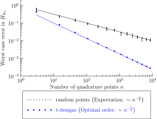
Figure 1: Random sampling according to $\mu_{2,4}$ vs. integration by $t$-desings.

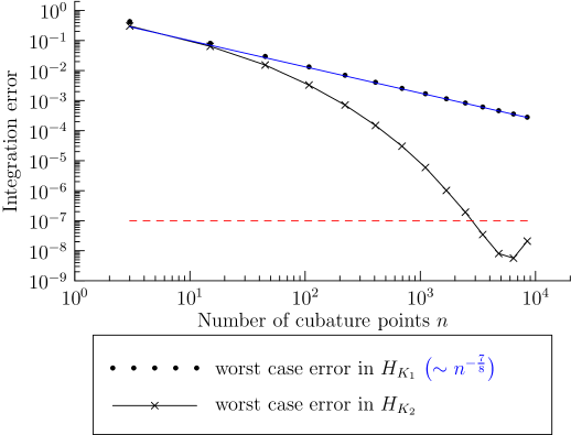
Figure 2: Integration of smooth vs. integration of nonsmooth functions.

5.2 Approximation

Similar, as in the previous section we aim to approximate a smooth and a nonsmooth function, namely

$$f_{1}(P)=K_{1}(I_{2},P),\qquad f_{2}(P)=K_{2}(I_{2},P),\qquad P\in\mathcal{G}_{2,4},$$

where $K_{1}$, $K_{2}$ are from the previous section and $I_{2}$ is a projection matrix with $2$ ones on the upper left diagonal. This time we observe that the function $f_{1}$ is contained in $H^{3}_{\infty}(\mathcal{G}_{2,4})$ but $f\not\in H^{3+\epsilon}_{\infty}(\mathcal{G}_{2,4})$, for all $\epsilon>0$. For the smooth function $f_{2}$, we have $f_{2}\in H^{s}_{\infty}(\mathcal{G}_{2,4})$, for any $s>0$.

Since the computed $t$-designs are with respect to $\operatorname{Pol}_{t}(\mathcal{G}_{2,4})$ and not $\Pi_{t}(\mathcal{G}_{2,4})$, we need an additional scaling of $s(t)$ in $\sigma_{t}$. According to Example 1, the choice

$$s(t)=\sqrt{2(t^{2}+3t+3+(-1)^{t})}-\epsilon\asymp t\sqrt{2},$$

for small $\epsilon>0$, yields $\Pi_{s(t)}\cdot\Pi_{s(t)}\subset\operatorname{Pol}_{2t}(\mathcal{G}_{2,4})$. For numerical experiments, we take $\epsilon$ to be smaller than the machine precision, so that it is effectively zero. Hence, in accordance with Theorem 3.3, we use the following kernel based approximation

$$\sigma_{s(t)}(f,X_{2t})=\frac{1}{n_{2t}}\sum_{j=1}^{n_{2t}}f(P_{j})\sum_{l(\pi)\leq 2}h(s(t)^{-2}\lambda(\pi))K_{\pi}(P_{j},\cdot),$$

where $X_{2t}=\{(P^{2t}_{j},1/n_{2t})\}_{j=1}^{n_{2t}}$ and

$$h(x)=\begin{cases}\big{(}1+\exp(\frac{3-4x}{2-6x+4x^{2}})\big{)}^{-1},&1/2<x<1,\\ 1,&x\leq 1/2,\\ 0,&\text{otherwise.}\end{cases}$$

The approximation error is determined by randomly sampling altogether $50000$ points. The first 25000 are pseudo random according to $\mu_{2,4}$. Since $f_{1}$ has a nonsmooth point at $I_{2}$ the maximal error is expected around this point. Therefore, we sampled the other $25000$ from normally distributed points around that point $I_{2}$ with variance $0.15$ and $0.5$ in the matrix entries, i.e., we choose $Z\in\mathbb{R}^{4\times 4}$ with independent and identically distributed entries according to a normal distribution with mean zero and variance $0.15$ and $0.5$, respectively, and then project $I_{2}+Z$ onto $\mathcal{G}_{2,4}$, which we accomplished by a QR-decomposition in Matlab.

In Figure 3, we can observe the predicted decay in Theorem 3.3 for the function $f_{1}\in H^{3}_{\infty}(\mathcal{G}_{2,4})$. Furthermore, as expected for the smooth function $f_{2}$, the error appears to decrease super linearly.

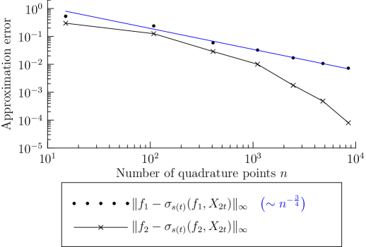
Figure 3: Approximation of a smooth vs. approximation of a nonsmooth function.

- (1) P.-A. Absil, R. Mahony, and R. Sepulchre, Optimization algorithms on matrix manifolds, Princeton University Press, 2008.
- (2) C. Bachoc, Linear programming bounds for codes in Grassmannian spaces, IEEE Trans. Inf. Th. 52 (2006), no. 5, 2111–2125.
- (3) C. Bachoc, E. Bannai, and R. Coulangeon, Codes and designs in Grassmannian spaces, Discrete Mathematics 277 (2004), 15–28.
- (4) C. Bachoc, R. Coulangeon, and G. Nebe, Designs in Grassmannian spaces and lattices, J. Algebraic Combinatorics 16 (2002), 5–19.
- (5) A. Bondarenko, D. Radchenko, and M. Viazovska, Optimal asymptotic bounds for spherical designs, Ann. Math. 178 (2013), no. 2, 443–452.
- (6) L. Brandolini, C. Choirat, L. Colzani, G. Gigante, R. Seri, and G. Travaglini, Quadrature rules and distribution of points on manifolds, Annali della Scuola Normale Superiore di Pisa - Classe di Scienze XIII (2014), no. 4, 889–923.
- (7) J. Brauchart, E. Saff, I. H. Sloan, and R. Womersley, QMC designs: Optimal order quasi Monte Carlo integration schemes on the sphere, Math. Comp. 83 (2014), 2821–2851.
- (8) Y. Chikuse, Statistics on special manifolds, Lecture Notes in Statistics, Springer, New York, 2003.
- (9) A. W. Davis, Spherical functions on the Grassmann manifold and generalized Jacobi polynomials – part 1, Lin. Alg. Appl. 289 (1999), no. 1-3, 75–94.
- (10) P. de la Harpe and C. Pache, Cubature formulas, geometrical designs, reproducing kernels, and Markov operators, Infinite groups: geometric, combinatorial and dynamical aspects (Basel), vol. 248, Birkhäuser, 2005, pp. 219–267.
- (11) I. Dumitriu, A. Edelman, and G. Shuman, MOPS: Multivariate orthogonal polynomials (symbolically), Journal of Symbolic Computation 42 (2007), no. 6, 587–620.
- (12) M. Ehler, F. Filbir, and H. N. Mhaskar, Locally learning biomedical data using diffusion frames, J. Comput. Biol. 19 (2012), no. 11, 1251–64.
- (13) M. Ehler and M. Gräf, Harmonic decompositions on unions of Grassmannians, arXiv (2016).
- (14) F. Filbir and H. N. Mhaskar, A quadrature formula for diffusion polynomials corresponding to a generalized heat kernel, J. Fourier Anal. Appl. 16 (2010), no. 5, 629–657.
- (15) , Marcinkiewicz–Zygmund measures on manifolds, J. Complexity 27 (2011), no. 6, 568–596.
- (16) D. Geller and I. Z. Pesenson, Band-limited localized Parseval frames and Besov spaces on compact homogeneous manifolds, J. Geom. Anal. 21 (2011), no. 2, 334–371.
- (17) , -widths and approximation theory on compact Riemannian manifolds, Commutative and Noncommutative Harmonic Analysis and Applications (A. Mayeli, P. E. T. Jorgensen, and G. Ólafsson, eds.), vol. 603, Contemporary Mathematics, 2013.
- (18) , Kolmogorov and linear widths of balls in Sobolev spaces on compact manifolds, Math. Scand. 115 (2014), no. 1, 96–122.
- (19) Q. T. Le Gia and H. N. Mhaskar, Polynomial operators and local approximation of solutions of pseudo-differential operators on the sphere, Numerische Mathematik 103 (2006), 299–322.
- (20) , Localized linear polynomial operators and quadrature formulas on the sphere, SIAM J. Numer. Anal. 47 (2008), no. 1, 440–466.
- (21) M. Gräf, Efficient algorithms for the computation of optimal quadrature points on Riemannian manifolds, Universitätsverlag Chemnitz, 2013.
- (22) L. Hörmander, The analysis of linear partial differential operators, I, II, III, IV, Springer Verlag, 1983-1985.
- (23) A. T. James and A. G. Constantine, Generalized Jacobi polynomials as spherical functions of the Grassmann manifold, Proc. London Math. Soc. 29 (1974), no. 3, 174–192.
- (24) M. Maggioni and H. N. Mhaskar, Diffusion polynomial frames on metric measure spaces, Appl. Comput. Harmon. Anal. 24 (2008), no. 3, 329–353.
- (25) H. N. Mhaskar, Eignets for function approximation on manifolds, Appl. Comput. Harmon. Anal. 29 (2010), 63–87.
- (26) E. Novak and H. Wozniakowski, Tractability of Multivariate Problems. Volume II, EMS Tracts in Mathematics, vol. 12, EMS Publishing House, Zürich, 2010.
- (27) I. Z. Pesenson and D. Geller, Cubature formulas and discrete fourier transform on compact manifolds, From Fourier Analysis and Number Theory to Radon Transforms and Geometry, vol. 28, 2012, pp. 431–453.
- (28) D. L. Ragozin, Polynomial approximation on compact manifolds and homogeneous spaces, Trans. Amer. Math. Soc. 150 (1970), 41–53.
- (29) P. Seymour and T. Zaslavsky, Averaging sets: a generalization of mean values and spherical designs, Advances in Math. 52 (1984), 213–240.
- (30) E. M. Stein, Singular integrals and differentiability properties of functions, Princeton University Press, 1970.
- (31) H. Triebel, Theory of Function Spaces II, Birkhäuser, Basel, 1992.