Toward a measurement of the effective gauge field and the Born-Huang potential
with atoms in chip traps
Zeynep Nilhan Gürkan
College of Engineering and Technology, American University of the Middle East, Egaila,
54200, Kuwait
Erik Sjöqvist
Department of Physics and Astronomy, Uppsala University, Box 516,
Se-751 20 Uppsala, Sweden
Björn Hessmo
Department of Applied Physics, Royal Institute of Technology, Se-106 91, Stockholm, Sweden
Centre for Quantum Technologies, National
University of Singapore, 2 Science Drive 3, 117542 Singapore
Benoît Grémaud
Aix Marseille Univ, Université de Toulon, CNRS, CPT, IPhU, AMUTech, Marseille, France
Centre for Quantum Technologies, National
University of Singapore, 2 Science Drive 3, 117542 Singapore
Abstract
We study magnetic traps with very high trap frequencies where the spin is coupled to the motion
of the atom. This allows us to investigate how the Born-Oppenheimer approximation fails and
how effective magnetic and electric fields appear as the consequence of the non-adiabatic
dynamics. The results are based on exact numerical diagonalization of the full Hamiltonian describing the coupling between the internal and external degrees of freedom. The position in energy and the decay rate of the trapping states correspond to the imaginary part of the resonances of this Hamiltonian are computed using the complex rotation method.
I Introduction
Magnetic trapping is one of the workhorses for cold atom physics. A commonly used
trap is the Ioffe-Pritchard trap pritchard1983 , in which the magnetic field is non-zero
at the center to prevent Majorana transitions to scattering states. In most situations,
it is highly desirable to obtain high trapping frequencies and gradients for fast thermalization
and strong confinement of the atoms. One method to reach high frequencies is to miniaturize
the magnetic trap by using microfabricated chips Fortagh2007 ; a widely used setup for studying adiabatic dynamics in atomic systems Lesa . This far most magnetic
traps operate in a regime where the atomic spin can adiabatically follow local changes in
the magnetic field. Before atoms are lost, the dynamics will be influenced by corrections to the adiabatic approximation. One such example would be where an atom orbits a current carrying wire. To describe losses and nonadiabatic effects in magnetic traps, it is convenient to work with waveguides to reduce the problem to two dimensionsAnglinSchmiedmayer ; Franzosi ; Hinds ; SchmiedScrinzi .
In this article, we analyze the situation in magnetic traps with very high trap frequencies,
where the spin is coupled to the motion of the atom. This allows us to investigate how
the Born-Oppenheimer approximation fails and how effective magnetic and electric fields
appear as a consequence of the non-adiabatic dynamics
Berry1990 ; mead1992 ; dalibard2011 ; goldman2014 . The results are based on exact numerical diagonalization of the full Hamiltonian describing the coupling between the internal and external degrees of freedom. Using the complex rotation method, the position in energy and the decay rate of the trapping states corresponding to the imaginary part of the resonances of this Hamiltonian are computed Buchl94 .
II Magnetic trapping
II.1 Atoms in a magnetic field
The Hamiltonian of an atom with mass and spin operator in a magnetic
field , is given by
(1)
where is the Bohr magneton and is the factor. We consider the
case. By writing
(2)
where , and values are varying in space, the Hamiltonian reads
(3)
(7)
in the eigenbasis of .
When the Larmor frequency is much larger than the
typical frequency of the atomic motion, the fast spin dynamics decouple from the slow
evolution of the center of mass of the atom. In the Born-Oppenheimer approximation,
the state of the system is written as
(8)
where is the wave function and is an eigenvector
of the position dependent spin-part of the Hamiltonian in Eq. (7). The effective
potential seen by the atoms is just the associated eigenvalue , whose minimum,
if existing, creates a trapping potential. In addition, since the local eigenstates
are position dependent a vector potential and an additional
scalar potential appear, for each component
:
(9)
These quantities are well-known in molecular physics as Berry-Mead and Born-Huang
potentials mead1992 . In cold atomic gases, they appear in the situation of position
dependent dark-states Rus , allowing experimental realizations of artificial
gauge fields Lin . The eigenstates of the spin Hamiltonian
are only defined up to a phase factor, which can be position dependent. From the preceding
expression, one readily obtains that the change amounts
to the gauge transformation:
(10)
In addition to these adiabatic terms, there are also couplings between the different eigenstates
, which appears as off-diagonal terms of the Hamiltonian in the
basis. They are precisely responsible for the Majorana losses
Suk ; Bri .
II.2 Experimental set-up
To observe the effects of the effective Berry-Mead and Born-Huang potentials, it is
required to use magnetic traps with high trap frequencies. One efficient way to realize this
is to use microfabricated magnetic traps, which are formed when the magnetic field from
a small current-carrying wire is superimposed with an external bias field. The magnetic field
from a thin and long wire along the - axis is given by , where is the polar angle in
cylindrical coordinates, is the distance from the wire, and is current. We assume a homogeneous
external bias field .
Superimposing and , we obtain, in cartesian coordinates,
the total magnetic field
(11)
The magnitude of is given by
(12)
with . This has a minimum at the position
, where weak-field seeking atoms can be trapped.
Introducing local coordinates around the minimum ,
the -components of the magnetic field read:
(13)
which to first order in and reduce to
(14)
This approximation can be readily obtained from the linearization of at the
minimum of the potential: , where is the gradient
of the magnetic field in the plane, i.e.,
(15)
II.3 Harmonic units
As explained just above, weak-field seeking atoms can be trapped around the minimum of the
magnetic field; more precisely, the effective trapping potential is proportional to:
(16)
where the harmonic approximation leads an effective trap frequency (and harmonic length)
(17)
Using and as harmonic units for length and energy and by introducing
the Larmor-type frequency , the Hamiltonian for a spin-
reads
(21)
where
(22)
We are now using the notation and for the scaled position around the minimum, not
to be confused with the original notation. In these rescaled units, one has .
With the above definition, it follows that
(23)
in terms of which
(24)
The ratio precisely compares the motional dynamics (frequency trap) to the spin dynamics
(Larmor frequency). As one can see, the full dynamics of the problem depend only on this single
dimensionless parameter. In the usual trapping situation, this is a small parameter, typically
ranging from to , telling that, (i) the Born-Oppenheimer approximation is
valid, and (ii) the trap is almost harmonic .
On the other hand, for , i.e., the timescale of the spin and the motional dynamics
are comparable, deviations from the harmonic behavior are marked and all the effects beyond
the Born-Oppenheimer approximation become important, in particular the Majorana’s losses.
Finally, as functions of the magnetic field gradient (in ) and the bias field
(in ), one has for Rb87:
(25)
For a given value of and , the dimensionfull
values for frequencies and the decay rates
are related to the numerical ones as follows:
(26)
see below for application.
III Beyond the Born-Oppenheimer approximation
III.1 Effective Hamiltonian
As mentioned above, beside the vector potentials and the Born-Huang scalar potentials
, off-diagonal couplings between the components arise because of the motion
of the atoms. From a mathematical point of view, this is nothing but saying that the operator
does not commute with the position dependent diagonalization of the
spin Hamiltonian. More precisely, decomposing the state of the system
in the eigenstates of the spin Hamiltonian, , one can derive the effective Hamiltonian acting
on the wave functions . One has
(27)
where the are the Zeeman states. The associated eigenvalues are ,
and , respectively.
Assuming that the magnetic field simply reads , one obtains
(28)
In the adiabatic limit,
i.e., , , the trapping state is
,
In harmonic units, acting on the vector
reads formally as follows:
(29)
The diagonal entries take the form
(30)
where
(31)
with and .
The off-diagonal entries of are
(32)
is Hermitian with respect to the scalar product .
III.2 Numerical implementation
The Hamiltonian is invariant under spatial rotations, therefore the eigenstates
can be written as . For each value of , the resulting
Hamiltonian only depends on the radial coordinate . Since the value of the functions
at is not fixed by any boundary condition, one uses a discretization scheme that
does not contain the point , namely the grid points are , for
ranging from to a maximum value . fixes the number of grid points per
harmonic length, whereas corresponds to the size of the system in harmonic length
units. The Hamiltonian is Hermitian for the scalar product , where ,
such that it is the discretization of the equation that leads to
a generalized eigenvalue problem , where and are
Hermitian matrices, being positive definite.
Neglecting the off-diagonal coupling, the effective potentials seen by and
components being and , the corresponding eigenstates are not bound states
but scattering states, whereas they are bound states for the component. The off-diagonal
coupling allows this bound states to decay to the scattering channels, which, from a mathematical
point of view, becomes resonances, i.e., complex poles of the Green function .
The complex rotation method is appropriate to compute directly the properties of these
resonances (energy, width). Its properties rely on mathematical properties of the analytic
continuation of the Green’s function in the complex plane Balslev71 ; Ho83 . A review of
its application to atomic physics can be found in Buchl94 .
The method is implemented in our case by making the radial coordinate complex:
and , where is a real parameter (the rotation angle).
The matrix representations of the Hamiltonian then become complex symmetric,
but are no more Hermitian. The fundamental properties of the complex spectra are :
•
The bound states, if any, are still on the real axis.
•
The continua are rotated by an angle on the lower-half complex
plane, around their branching point.
•
Each complex eigenvalue gives the properties of one resonance, i.e.,
the energy is the real part of , and the width is two times the negative
of the imaginary part. The complex eigenvalues are independent of ,
provided that they are not covered by the continua.
Note that in the present case, the branching point associated to is located at
, whereas the one associated to is formally at , since
for large . The scattering states for a linear potential oscillate faster
for large distance, such that they cannot be accurately described within a discretization
scheme. On the other hand, the overlap with the bound states at very large distance is
negligible, so that the exact behavior barely impacts the position and the width of the
resonance. Therefore to avoid numerical artifacts and increase the numerical accuracy,
we replace the anti-trapping potential for by
(33)
where is a small parameter, typically . For , then
, whereas for , then , such that the scattering states have a well defined wavelength for large
values. We have numerically checked that the results presented here are insensitive to
the actual value.
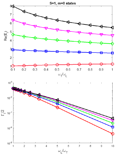
III.3 Results
The properties of the resonances (position in energy and width) are displayed, as functions of
, in Fig. 1 for the states and in Fig. 2
for the states. In both cases, the zero of energy corresponds to the bottom of the
trapping state, i.e., corresponding to a global shift of of the eigenenergies
of , such that in the adiabatic limit , the energies directly
correspond to the harmonic oscillator levels. This is clearly seen on the left part of the top plots.
On the contrary, for (right part), the energy levels differ from the harmonic
one, in particular, the difference in energy gets smaller with higher reflecting
the linear behavior of the trapping potential at large . The behavior in the adiabatic
regime can be obtained from the perturbation expansion of with respect to
and . More precisely, for a fixed value of , reads:
(34)
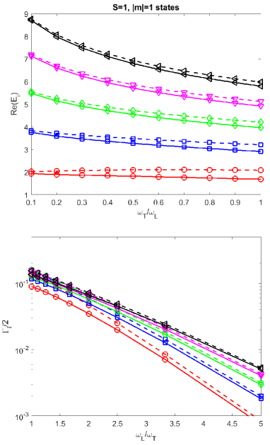
where when .
The second term arises from the gauge field and results in a energy
splitting among the states, which is clearly observed in Fig. 2. A Taylor expansion
of these two terms at small distances leads respectively to:
(35)
The two terms proportional to correspond to an energy shift whereas the two terms
proportional to correspond to modification of the trap frequency. However, the
preceding formula cannot be compared directly to the numerical results since at large distances
, the two last terms in leads to an effective centrifugal potential
, which is independent of . This shows that, although
and are
small perturbations to the , the resulting energy shift has to be computed using their
exact expressions, not just their Taylor expansion around . Furthermore, in the adiabatic regime, the decay rates can be obtained from the Fermi golden
rule. Assuming that one can approximate the scattering states as plane waves , i.e., neglecting the fact that is a radial coordinate, the decay rates are
proportional to the modulus square of the Fourier transform of the
harmonic trap wave functions, taken at the corresponding to the energy of the bound state,
i.e., such that . At first order the decay is dominated by
the Gaussian decay of the wave function , such that one has:
(36)
Therefore, one predicts a linear behavior of as functions of . This can be seen for both and states
(Figs. 1 and 2, bottom plots).
Figure 1: (color online) Properties of the resonances of the Hamiltonian
: positions in energy as functions of (top plot) and decay rates as functions of (bottom plot). A given symbol and color correspond to the same state for the
two plots.
Figure 2: (color online) Properties of the resonances of the Hamiltonian
: positions in energy as functions of (top plot)
and decay rates as functions of (bottom plot). The dashed line is for and the solid line is for . A given symbol and color correspond to the same state for the
two plots.
The behavior, at fixed , is slightly more complicated since one has to
take into account the exact shape of the harmonic functions, in particular to explain that for
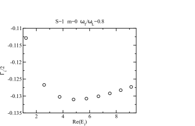
small , the decay rates increase with the principal quantum number. We have checked on a simpler model that it is indeed a generic behavior: for a fixed value
of , the decay rates depict a maximum around an energy (which depends on ),
see Fig. 3.
From the numerical point of view, Table 1 summarizes the expected decay rate
of the ground state and the energy splitting between the first two states
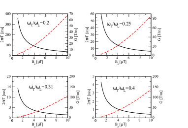
for few values of . From the experimental point of view, for Rb87 Fig. 4
displays the life-time (solid black line) and the gradient (red dashed line)
as functions of the bias field along the axis, for the four different values of
depicted in Table 1. For instance, for a value of
(top-left plot), for a bias field value of , the
life-time is ms, whereas is . For these values, the trap
frequency is kHz. The energy splitting between the states is kHz.
The splitting of the energy levels can be measured using RF-spectroscopy on the magnetic
trap for a cold thermal cloud Martin1988 .
0.2
0.25
0.31
0.4
0.15
0.18
0.21
0.25
Table 1: Decay rate of the ground state and the energy splitting between the
first two states for four values of .
Figure 3: Resonances in the complex energy plane for a fixed value
of . As one can see, around an energy value that depends on , for , the imaginary part of the resonances attains a (negative) minimum value, corresponding therefore to a maximum value of the decay rate.
Figure 4: (color online) Lifetime (solid black line, left axis) and the gradient
(red dashed line, right axis) as functions of the bias field along the axis, for the four
different values of depicted in the Table 1. For instance,
for a value of (top-left plot), for a bias field value of ,
the life-time is ms, whereas is . For this value, the trap
frequency is kHz. The energy splitting between the states is
kHz.
IV Conclusions
We have shown that a tight magnetic trap allows for investigating the break-down of the Born-Oppenheimer
condition. For instance, the adiabatic corrections reduce trap frequencies and the Born-Huang
potential counteracts the adiabatic potential. The coupling between trapping and anti-trapping states results in losses which, nevertheless remain experimentally tolerable. In addition, we have shown how molecular Aharonov-Bohm gauge potentials responsible for topological Berry phase effects are emerging. These effects are two-dimensional analogues of the Weyl cones that have been simulated in cold atoms Suc06 .
Within experimentally accessible parameter ranges, i.e reasonable , one
could measure Majorana losses and the splitting between , due to Berry connection
and Born-Huang terms characterizing thereby their impact.
As a future work, one could study the dynamics of a wave packet, for instance shifting the
trap center. Finally, it would be interesting to study the impact of atom-atom interactions.
Acknowledgments
The Centre for Quantum Technologies is a Research Centre of Excellence funded by the
Ministry of Education and National Research Foundation of Singapore. E. S. acknowledges financial support from the Swedish
Research Council (VR) through Grant No. D0413201. The project leading to this publication has received
funding from Excellence Initiative of Aix-Marseille Uni-
versity - A*MIDEX, a French “Investissements d’Avenir”
program through the IPhU (AMX-19-IET-008) and
AMUtech (AMX-19-IET-01X) institutes.
References
(1) D. Pritchard,
Phys. Rev. Lett. 51, 1336 (1983).
(2) J. Fortagh, C. Zimmermann,
Rev. Mod. Phys. 79, 235 (2007).
(3) I. Lesanovsky, T. Schumm, S. Hofferberth, L.M. Andersson, P. Krüger, and J. Schmiedmayer, Phys. Rev. A 73,
033619 (2006).
(4) J. R. Anglin, J. Schmiedmayer,
Phys. Rev. A 69, 022111 (2004).
(5)R. Franzosi, B. Zambon, E. Arimondo,
Phys. Rev. A 70, 053603 (2004).
(6) E. A. Hinds, C. Eberlein,
Phys. Rev. A 61, 033614 (2000).
(7) J. Schmiedmayer, A. Scrinzi,
Quantum Semiclass. Opt. 8, 693 (1996).
(8) M. V. Berry, R. Lim,
J. Phys. A: Math. Gen. 23, 655 (1990).
(9) C. A. Mead,
Rev. Mod. Phys. 64, 51 (1992).
(10) J. Dalibard, F. Gerbier, G. Juzeliunas, P. Öhberg, I. B. Spielman
Rev. Mod. Phys. 83, 1523 (2011).
(11) N. Goldman, G. Juzeliunas,P. Öhberg,
Rep. Prog. Phys. 77, 126401 (2014).
(12) A. Buchleitner, B. Grémaud,D. Delande,
J. Phys. B: At. Mol. Opt. Phys. 27, 2663 (1994).
(13) J. Ruseckas, G. Juzeliunas, P. Öhberg, M. Fleischauer,
Phys. Rev. Lett. 95, 010404 (2005).
(14) Y. -J. Lin, K. Jiménez-García, I. B. Spielman,
Nature (London), 471, 83 (2011).
(15) C. V. Sukumar, D. M. Brink, Phys. Rev. A 56, 2451 (1997)
(16) D. M. Brink, C. V. Sukumar, Phys. Rev. A 74, 035401 (2006)
(17) E. Balslev, J. M. Combes,
Commun. Math. Phys. 22, 280 (1971).
(18) Y. K. Ho,
Phys. Rep. 99, 1 (1983).
(19) A. G. Martin, K. Helmerson, V. S. Bagnato, G. P. Lafyatis, D. E. Pritchard,
Phys. Rev. Lett. 61, 2431 (1988).