Phase transition and thermodynamic geometry of $f(R)$ AdS black holes in the grand canonical ensemble

Abstract

The phase transition of four-dimensional charged AdS black hole solution in the $R+f(R)$ gravity with constant curvature is investigated in the grand canonical ensemble, where we find novel characteristics quite different from that in canonical ensemble. There exists no critical point for $T-S$ curve while in former research critical point was found for both the $T-S$ curve and $T-r_{+}$ curve when the electric charge of $f(R)$ black holes is kept fixed. Moreover, we derive the explicit expression for the specific heat, the analog of volume expansion coefficient and isothermal compressibility coefficient when the electric potential of $f(R)$ AdS black hole is fixed. The specific heat $C_{\Phi}$ encounters a divergence when $0<\Phi<b$ while there is no divergence for the case $\Phi>b$. This finding also differs from the result in the canonical ensemble, where there may be two, one or no divergence points for the specific heat $C_{Q}$. To examine the phase structure newly found in the grand canonical ensemble, we appeal to the well-known thermodynamic geometry tools and derive the analytic expressions for both the Weinhold scalar curvature and Ruppeiner scalar curvature. It is shown that they diverge exactly where the specific heat $C_{\Phi}$ diverges.

I Introduction

$f(R)$ gravity has various applications in both gravitation and cosmology. For example, it mimics the cosmological history successfully. One can read the nice reviews Felice ; Capozziello ; Odintsov1 to gain an comprehensive understanding. Believing that black holes in $f(R)$ gravity distinguish from those in Einstein gravity, both the black hole solutions in $f(R)$ gravity and their thermodynamics Dombriz -xiong6 have received considerable attention.

In our recent paper xiong6 , we investigated the phase transition of four-dimensional charged AdS black hole solution in the $R+f(R)$ gravity with constant curvature Moon98 in the canonical ensemble. To provide a consistent and unified picture of its critical phenomena, we studied not only the critical point of $T-S$ curve and $T-r_{+}$ curve, but also the divergent behavior of specific heat at constant charge and scalar curvature of Quevedo’s geometrothermodynamics Quevedo2 .

In this paper, we would like to generalize our recent research xiong6 to the grand canonical ensemble. This generalization is of interest and it is believed that the phase transition in the grand canonical ensemble will behave quite differently from that in the canonical ensemble, which has been witnessed in our former research of charged topological black holes in Hořava-Liftshitz gravity jiexiong1 and Lovelock Born-Infeld gravity jiexiong2 and has also been witnessed in many other references. So the motivation is to probe novel characteristics of phase transition for four-dimensional charged AdS black hole solution in the $R+f(R)$ gravity with constant curvature from the perspective of grand canonical ensemble. Our research will also disclose interesting properties due to $f(R)$ gravity.

The organization of this paper is as follows. In Sec. II we will review briefly four-dimensional charged AdS black hole solution in the $R+f(R)$ gravity with constant curvature. In Sec. III we will investigate the behavior of temperature and phase transition in grand canonical ensemble. In Sec. IV, we will study both the Weinhold thermodynamic geometry Weinhold and Ruppeiner thermodynamic geometry Ruppeiner in grand canonical ensemble. Conclusions will be drawn in Sec. V.

II Review of black hole solution in the $R+f(R)$ gravity with constant curvature

In Ref. Moon98 , four-dimensional charged AdS black hole solution in the $R+f(R)$ gravity with constant curvature was obtained with its thermodynamic quantities, such as energy, entropy, heat capacity and Helmhotz free energy discussed. $P-V$ criticality of this solution was investigated in Ref. Chen . Recently, we investigated the coexistence curve and the number densities of black hole molecules for this black hole solution xiong5 and studied its phase transition in the canonical ensemble when the charge of the black hole is fixed xiong6 .

The corresponding black hole solution reads Moon98

$$ds^{2}=-N(r)dt^{2}+\frac{dr^{2}}{N(r)}+r^{2}(d\theta^{2}+sin^{2}\theta d\phi^{2}),$$ (1)

where

$$N(r) = 1-\frac{2m}{r}+\frac{q^{2}}{br^{2}}-\frac{R_{0}}{12}r^{2},$$ (2)

$$b = 1+f^{\prime}(R_{0}).$$ (3)

In the above solution, $b>0,R_{0}<0$. Note that the black hole solution reduces to RN-AdS black hole when $b=1,R_{0}=-12/l^{2}$.

The black hole ADM mass $M$ and the electric charge $Q$ are related to the parameters $m$ and $q$ respectively as Moon98

$$M=mb,\;\;\;Q=\frac{q}{\sqrt{b}}.$$ (4)

Its thermodynamic quantities were reviewed in Ref. Chen as follows

$$T = \frac{N^{\prime}(r_{+})}{4\pi}=\frac{1}{4\pi r_{+}}(1-\frac{q^{2}}{br_{+}^{2}}-\frac{R_{0}r_{+}^{2}}{4}).$$ (5)

$$S = \pi r_{+}^{2}b.$$ (6)

$$\Phi = \frac{\sqrt{b}q}{r_{+}}.$$ (7)

$T$, $S$ and $\Phi$ denote the Hawking temperature, the entropy and the electric potential respectively. Note that the entropy here was derived from the Wald method Moon98 ; Felice . Readers who are interested in it can further read Section 13.2 of reference Felice and the famous literature Wald .

III Phase transition of $f(R)$ AdS black hole in grand-canonical ensemble

To facilitate the calculation of relevant quantities, it is convenient to reexpress the Hawking temperature as the function of entropy and electric potential

$$T=\frac{4b^{2}\pi-bR_{0}S-4\pi\Phi^{2}}{16\pi^{3/2}b^{3/2}\sqrt{S}}.$$ (8)

When $b=1,R_{0}=-12/l^{2}=4\Lambda$, Eq.(8) reduces to

$$T=\frac{\pi-\Lambda S-\pi\Phi^{2}}{4\pi^{3/2}\sqrt{S}},$$ (9)

which is in accord with the result of RN-AdS black holes Banerjee1 ; Banerjee2 .

With Eq.(8), it is quite easy to obtain

$$\left(\frac{\partial T}{\partial S}\right)_{\Phi} = \frac{-b(4b\pi+R_{0}S)+4\pi\Phi^{2}}{32\pi^{3/2}(bS)^{3/2}},$$ (10)

$$\left(\frac{\partial^{2}T}{\partial S^{2}}\right)_{\Phi} = \frac{12b^{2}\pi+bR_{0}S-12\pi\Phi^{2}}{64\pi^{3/2}b^{3/2}S^{5/2}}.$$ (11)

The solution for $\left(\frac{\partial T}{\partial S}\right)_{\Phi}=0$ can be derived as

$$S_{1}=\frac{-4\pi(b^{2}-\Phi^{2})}{bR_{0}}.$$ (12)

Note that $b>0,R_{0}<0$, the condition $0<\Phi<b$ should be satisfied to ensure that the entropy in Eq.(12) is positive. For the case $\Phi>b$, no meaningful root satisfies the equation $\left(\frac{\partial T}{\partial S}\right)_{\Phi}=0$. Substituting Eq.(12) into (11), one can obtain that

$$\left(\frac{\partial^{2}T}{\partial S^{2}}\right)_{\Phi}\mid_{S=S_{1}}=\frac{bR_{0}^{4}}{256\pi^{3}[R_{0}(-b^{2}+\Phi^{2})]^{3/2}}>0.$$ (13)

So there is no critical point for $T-S$ curve. This finding differs from our former research, where we found critical point for both the $T-S$ curve and $T-r_{+}$ curve when the electric charge of $f(R)$ black holes is kept fixed xiong6 , providing one more example that the thermodynamics in the grand canonical ensemble is quite different from that in the canonical ensemble.

The Hawking temperature for both the case $0<\Phi<b$ and $\Phi>b$ is depicted in Fig. 1 and  1 respectively. As shown in Fig. 1, there exists minimum temperature when $0<\Phi<b$. Substituting Eq.(12) into Eq.(8), the minimum temperature can be obtained as

$$T_{min}=\frac{\sqrt{-R_{0}(b^{2}-\Phi^{2})}}{4b\pi}.$$ (14)

However, the Hawking temperature increases monotonically when $\Phi>b$, as can be witnessed in Fig. 1.

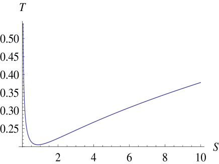
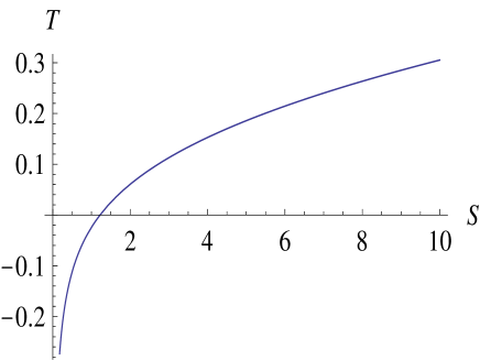
Figure 1: (a)Hawking temperature $T$ vs. $S$ for $b=1.5,\Phi=1,R_{0}=-12$ (b)Hawking temperature $T$ vs. $S$ for $b=1.5,\Phi=2,R_{0}=-12$;

When the electric potential of $f(R)$ AdS black hole is fixed, the specific heat can be derived as

$$C_{\Phi}=T(\frac{\partial S}{\partial T})_{\Phi}=\frac{2S(-4b^{2}\pi+bR_{0}S+4\pi\Phi^{2})}{4b^{2}\pi+bR_{0}S-4\pi\Phi^{2}}.$$ (15)

Note that the denominator of Eq.(15) is exactly the same as the numerator of Eq.(10), implying that the divergence of $C_{\Phi}$ corresponds to the minimum Hawking temperature.

When $b=1,R_{0}=-12/l^{2}=4\Lambda$, Eq.(15) reduces to

$$C_{\Phi}=\frac{2S[\pi(1-\Phi^{2})-\Lambda S]}{-\Lambda S-\pi(1-\Phi^{2})},$$ (16)

reproducing the result of RN-AdS black holes Banerjee1 .

Substituting Eq.(6) into Eq.(15), one can express the specific heat into the function of $r_{+}$ as

$$C_{\Phi}=\frac{2br_{+}^{2}(-4b^{2}\pi+bR_{0}\pi r_{+}^{2}+4\pi\Phi^{2})}{4b^{2}+b^{2}R_{0}r_{+}^{2}-4\Phi^{2}}.$$ (17)

One can also derive the analog of volume expansion coefficient and isothermal compressibility coefficient as

$$\alpha = \frac{1}{Q}(\frac{\partial Q}{\partial T})_{\Phi}=\frac{-16b^{2}\pi r_{+}}{4b^{2}+b^{2}R_{0}r_{+}^{2}-4\Phi^{2}},$$ (18)

$$\kappa_{T} = \frac{1}{Q}(\frac{\partial Q}{\partial\Phi})_{T}=\frac{4b^{2}+b^{2}R_{0}r_{+}^{2}-12\Phi^{2}}{\Phi(4b^{2}+b^{2}R_{0}r_{+}^{2}-4\Phi^{2})}.$$ (19)

Comparing Eqs.(18) and (19) with Eq.(17), one can find that both $\alpha$ and $\kappa_{T}$ share the same factor $4b^{2}+b^{2}R_{0}r_{+}^{2}-4\Phi^{2}$ in their denominators as the specific heat.

It is not difficult to find the condition corresponding to the divergence of $C_{\Phi}$, $\alpha$ and $\kappa_{T}$ as

$$4b^{2}+b^{2}R_{0}r_{+}^{2}-4\Phi^{2}=0,$$ (20)

which can be analytically solved as

$$r_{+}=\frac{2}{b}\sqrt{\frac{\Phi^{2}-b^{2}}{R_{0}}}.$$ (21)

Considering the restrictions $b>0,R_{0}<0$, the above root make sense physically only when $0<\Phi<b$.

Fig. 2 shows the case of $0<\Phi<b$ while Fig. 2 shows the case of $\Phi>b$. One can see clearly that the specific heat $C_{\Phi}$ encounters a divergence when $0<\Phi<b$ while there is no divergence for the case $\Phi>b$. This finding also differs from our former research in the canonical ensemble xiong6 , where there may be two, one or no divergence points for the specific heat $C_{Q}$.

Fig. 2 and  2 show that $\alpha$ and $\kappa_{T}$ diverge at the same place where $C_{\Phi}$ does, in accordance with the above deductions.

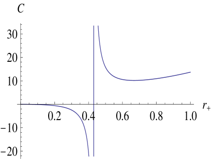
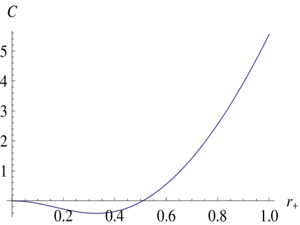
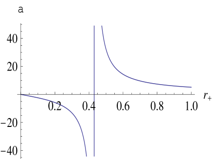
Figure 2: (a) $C_{\Phi}$ vs. $r_{+}$ for $R_{0}=-12,b=1.5,\Phi=1$ (b) $C_{\Phi}$ vs. $r_{+}$ for $R_{0}=-12,b=1.5,\Phi=2$ (c) $\alpha$ vs. $r_{+}$ for $R_{0}=-12,b=1.5,\Phi=1$ (d) $\kappa_{T}$ vs. $r_{+}$ for $R_{0}=-12,b=1.5,\Phi=1$

IV Thermodynamic geometry of $f(R)$ AdS black hole

To examine the phase structure newly found in Sec. III, we would like to appeal to thermodynamic geometry tools, such as Weinhold geometry Weinhold and Ruppeiner geometry Ruppeiner , which has found various applications in probing the phase structures of black holes Ruppeiner2 -jiexiong3 .

Weinhold’s metric Weinhold was proprosed as

$$g_{ij}^{W}=\frac{\partial^{2}U(x^{i})}{\partial x^{i}\partial x^{j}}.$$ (22)

Utilizing Eqs.(2), (4) and (6), one can express the mass of the black hole as the function of $S$ and $Q$ as

$$M=\frac{12b^{2}\pi^{2}Q^{2}+12b\pi S-R_{0}S^{2}}{24\pi^{3/2}\sqrt{bS}}.$$ (23)

Then the components of Weinhold’s metric can be calculated as

$$g_{SS}^{W} = \frac{12b^{2}\pi^{2}Q^{2}-4b\pi S-R_{0}S^{2}}{32\pi^{3/2}S^{5/2}\sqrt{b}},$$ (24)

$$g_{QQ}^{W} = \frac{b^{3/2}\sqrt{\pi}}{\sqrt{S}},$$ (25)

$$g_{SQ}^{W} = g_{QS}^{W}=\frac{-b^{3/2}\sqrt{\pi}Q}{2S^{3/2}}.$$ (26)

And Weinhold scalar curvature can be obtained via programming as

$$R^{W}=\frac{8\pi^{3/2}S^{3/2}\sqrt{b}\left[96b^{3}\pi^{3}Q^{2}-4b^{2}\pi^{2}(8+Q^{2}R_{0})S-20b\pi R_{0}S^{2}-3R_{0}^{2}S^{3}\right]}{(4b^{2}\pi^{2}Q^{2}-4b\pi S-R_{0}S^{2})^{3}},$$ (27)

which can be reexpressed into the function of $\Phi$ as

$$R^{W}=\frac{8b^{5}(4+r_{+}^{2}R_{0})(8+3r_{+}^{2}R_{0})+32b^{3}(-24+r_{+}^{2}R_{0})\Phi^{2}}{r_{+}(4b^{2}+b^{2}r_{+}^{2}R_{0}-4\Phi^{2})^{3}}.$$ (28)

Comparing Eq.(28) with Eq.(17), one may find that Weinhold scalar curvature shares the same factor $4b^{2}+b^{2}r_{+}^{2}R_{0}-4\Phi^{2}$ in the denominator as the specific heat does, implying it would diverge exactly where the specific heat diverges. This is also shown intuitively in Fig. 3.

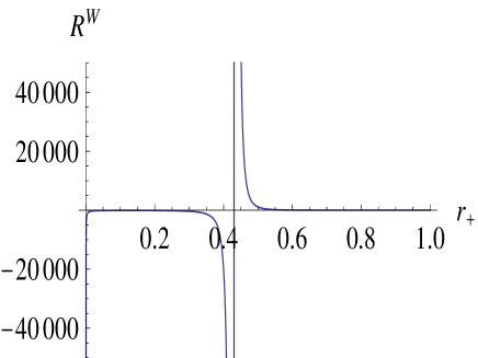
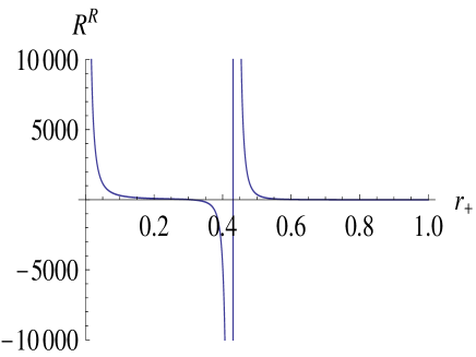
Figure 3: (a)Weinhold scalar curvature $R$ vs. $r_{+}$ for $b=1.5,\Phi=1,R_{0}=-12$ (b)Ruppeiner scalar curvature $R$ vs. $r_{+}$ for $b=1.5,\Phi=1,R_{0}=-12$;

Since the Ruppeiner’s metric is conformally connected to the Weinhold’s metric through the map Janyszek

$$dS^{2}_{R}=\frac{dS^{2}_{W}}{T}.$$ (29)

it is convenient to derive the components of Ruppeiner’s metric from those of Weinhold’s metric. They can be calculated as

$$g_{MM}^{R} = \frac{-12b^{2}\pi^{2}Q^{2}+4b\pi S+R_{0}S^{2}}{2S(4b^{2}\pi^{2}Q^{2}-4b\pi S+R_{0}S^{2})},$$ (30)

$$g_{QQ}^{R} = \frac{-16b^{2}\pi^{2}S}{4b^{2}\pi^{2}Q^{2}-4b\pi S+R_{0}S^{2}},$$ (31)

$$g_{MQ}^{R} = g_{QM}^{R}=\frac{8b^{2}\pi^{2}Q}{4b^{2}\pi^{2}Q^{2}-4b\pi S+R_{0}S^{2}}.$$ (32)

When $b=1,R_{0}=-12/l^{2}=4\Lambda$, Eqs.(30)-(32) reduces to

$$g_{MM}^{R} = \frac{-3\pi^{2}Q^{2}+\pi S+\Lambda S^{2}}{2S(\pi^{2}Q^{2}-\pi S+\Lambda S^{2})},$$ (33)

$$g_{QQ}^{R} = \frac{-4\pi^{2}S}{\pi^{2}Q^{2}-\pi S+\Lambda S^{2}},$$ (34)

$$g_{MQ}^{R} = g_{QM}^{R}=\frac{2\pi^{2}Q}{\pi^{2}Q^{2}-\pi S+\Lambda S^{2}},$$ (35)

which are equivalent to that in literature Banerjee2 of RN-AdS black holes .

Ruppeiner scalar curvature can be derived via programming as

$$R^{R}=\frac{A(S,Q)}{(4b^{2}\pi^{2}Q^{2}-4b\pi S-R_{0}S^{2})^{3}(4b^{2}\pi^{2}Q^{2}-4b\pi S+R_{0}S^{2})},$$ (36)

where

$$A(S,Q) = -1280b^{7}\pi^{7}Q^{6}+64b^{6}\pi^{6}Q^{4}(8-7Q^{2}R_{0})S+128b^{5}\pi^{5}Q^{2}(6+Q^{2}R_{0})S^{2}+16b^{4}\pi^{4}Q^{2}R_{0}(20-3Q^{2}R_{0})S^{3}$$ (37)

$$-336b^{3}\pi^{3}Q^{2}R_{0}^{2}S^{4}+4b^{2}\pi^{2}R_{0}^{2}(4-9Q^{2}R_{0})S^{5}+16b\pi R_{0}^{3}S^{6}+3R_{0}^{4}S^{7}.$$

It can be reexpressed into the function of $\Phi$ as

$$R^{R}=\frac{B(r_{+},\Phi)}{\pi r_{+}^{2}(4b^{2}+b^{2}r_{+}^{2}R_{0}-4\Phi^{2})^{3}(-4b^{2}+b^{2}r_{+}^{2}R_{0}+4\Phi^{2})},$$ (38)

where

$$B(r_{+},\Phi) = -b^{7}r_{+}^{4}R_{0}^{2}(4+r_{+}^{2}R_{0})(4+3r_{+}^{2}R_{0})+4b^{5}\Phi^{2}[-192+r_{+}^{2}R_{0}(-80+84r_{+}^{2}R_{0}+9r_{+}^{4}R_{0}^{2})]$$ (39)

$$+16b^{3}\Phi^{4}[-32+r_{+}^{2}R_{0}(-8+3r_{+}^{2}R_{0})]+64b\Phi^{6}(20+7r_{+}^{2}R_{0}).$$

Comparing Eq.(38) with Eq.(17), one may find that Ruppeiner scalar curvature shares the same factor $4b^{2}+b^{2}r_{+}^{2}R_{0}-4\Phi^{2}$ in the denominator as the specific heat does, implying it would diverge where the specific heat diverges. It can also be witnessed from Fig. 3. Our study of $f(R)$ AdS black holes proves again the Ruppeiner metric provides a excellent tool to probe the phase structures of black holes.

V Conclusions

In this paper, we investigate the phase transition of four-dimensional charged AdS black hole solution in the $R+f(R)$ gravity with constant curvature in the grand canonical ensemble. It is shown that the thermodynamics in the grand canonical ensemble is quite different from that in canonical ensemble xiong6 . There exists minimum temperature when $0<\Phi<b$ while the Hawking temperature increases monotonically when $\Phi>b$. There is no critical point for $T-S$ curve, differing from the result in canonical ensemble, where we found critical point for both the $T-S$ curve and $T-r_{+}$ curve when the electric charge of $f(R)$ black holes is kept fixed xiong6 .

Moreover, we derive the explicit expression for the specific heat, the analog of volume expansion coefficient and isothermal compressibility coefficient when the electric potential of $f(R)$ AdS black hole is fixed. They share the same factor $4b^{2}+b^{2}r_{+}^{2}R_{0}-4\Phi^{2}$ in the denominator and thus share the same divergent point. The specific heat $C_{\Phi}$ encounters a divergence when $0<\Phi<b$ while there is no divergence for the case $\Phi>b$. This finding also differs from the result in the canonical ensemble xiong6 , where there may be two, one or no divergence points for the specific heat $C_{Q}$.

To examine the phase structure of $f(R)$ AdS black hole newly found in the grand canonical ensemble, we appeal to thermodynamic geometry tools which has found various applications in probing the phase structures of black holes. We derive the analytic expressions for both the Weinhold scalar curvature and Ruppeiner scalar curvature. It is shown that they diverge exactly where the specific heat $C_{\Phi}$ diverges, proving again the Ruppeiner metric provides a excellent tool to probe the phase structures of black holes.

References

- (1) A. De Felice and S. Tsujikawa, theories, Living Rev. Rel. 13 (2010) 3
- (2) S. Capozziello and M. De Laurentis, Extended Theories of Gravity, Phys. Rept. 509 (2011) 167-321
- (3) S. Nojiri and S. D. Odintsov, Unified cosmic history in modified gravity: from theory to Lorentz non-invariant models, Phys. Rept. 505 (2011) 59-144
- (4) A. de la C. Dombriz, A. Dobado and A.L. Maroto, Black Holes in theories, Phys. Rev. D 80(2009)124011
- (5) T. Moon, Y. S. Myung and E. J. Son, Black holes, Gen. Rel. Grav. 43(2011)3079-3098.
- (6) A. Larranaga, A Rotating Charged Black Hole Solution in Gravity, Pramana 78(2012)697-703
- (7) J. A. R. Cembranos, A. de la C. Dombriz and P. J. Romero, Kerr-Newman black holes in f(R) theories, Int. J. Geom. Meth. Mod. Phys. 11(2014)1450001
- (8) A. Sheykhi, Higher-dimensional charged black holes, Phys. Rev. D 86(2012)024013
- (9) L. Sebastiani and S. Zerbini, Static Spherically Symmetric Solutions in Gravity, Eur. Phys. J. C 71(2011)1591
- (10) S. H. Hendi, The Relation between gravity and Einstein-conformally invariant Maxwell source, Phys. Lett. B 690(2010)220-223
- (11) S. H. Hendi and D. Momeni, Black hole solutions in gravity with conformal anomaly, Eur. Phys. J. C71(2011)1823
- (12) G. J. Olmo and D. R. Garcia, Palatini Black Holes in Nonlinear Electrodynamics, Phys. Rev. D 84(2011)124059
- (13) S. H. Mazharimousavi and M. Halilsoy, Black hole solutions in gravity coupled with non-linear Yang-Mills field, Phys. Rev. D 84(2011)064032
- (14) S. Chen, X. Liu, C. Liu and J. Jing, criticality of AdS black hole in gravity, Chin. Phys. Lett. 30(2013)060401
- (15) S. Nojiri and S. D. Odintsov, Instabilities and anti-evaporation of Reissner-Nordström black holes in modified gravity, Phys. Lett. B735 (2014) 376-382
- (16) S. Nojiri and S. D. Odintsov, Anti-Evaporation of Schwarzschild-de Sitter Black Holes in gravity, Class. Quant. Grav. 30(2013)125003
- (17) J. X. Mo and G. Q. Li, Coexistence curves and molecule number densities of AdS black holes in the reduced parameter space, Phys. Rev. D92 (2015)024055
- (18) J. X. Mo, G. Q. Li and Y. C. Wu, A consistent and unified picture for critical phenomena of f(R) AdS black holes, JCAP04(2016)045
- (19) H. Quevedo, Geometrothermodynamics, J. Math. Phys. 48(2007)013506
- (20) J. X. Mo, X. X. Zeng, G. Q. Li, X. Jiang and W. B. Liu, A unified phase transition picture of the charged topological black hole in Horava-Lifshitz gravity, JHEP 1310 (2013) 056
- (21) J. X. Mo and W. B. Liu, Non-extended phase space thermodynamics of Lovelock AdS black holes in the grand canonical ensemble, Eur. Phys. J. C75 (2015)211
- (22) F. Weinhold, Metric geometry of equilibrium thermodynamics, Chem. Phys. 63(1975)2479
- (23) G. Ruppeiner, A Riemannian geometric model, Phys. Rev. A 20(1979)1608
- (24) R. M. Wald, Black hole entropy is the Noether charge, Phys. Rev. D, 48(1993)3427 C3431
- (25) H. Janyszek, R. Mrugala, Geometrical structure of the state space inclassical statistical and phenomenological thermodynamics, Rep. Math. Phys. 27 (1989)145
- (26) G. Ruppeiner, Thermodynamic curvature and black holes, arXiv:1309.0901.
- (27) R. Tharanath, J. Suresh, N. Varghese and V. C. Kuriakose, Thermodynamic Geometry of Reissener-Nordström-de Sitter black hole and its extremal case, arXiv:1404.6789.
- (28) J. Suresh, R. Tharanath, N. Varghese and V. C. Kuriakose, The thermodynamics and thermodynamic geometry of the Park black hole, Eur. Phys. J. C 74 (2014) 2819.
- (29) S. A. H. Mansoori, B. Mirza, Correspondence of phase transition points and singularities of thermodynamic geometry of black holes, Eur. Phys. J. C 74 (2014) 2681.
- (30) M. B. J. Poshteh, B. Mirza, Z. Sherkatghanad, Phase transition, critical behavior, and critical exponents of Myers-Perry black holes, Phys. Rev. D 88 (2013) 024005
- (31) S. W. Wei and Y. X. Liu, Critical phenomena and thermodynamic geometry of charged Gauss-Bonnet AdS black holes Phys. Rev. D 87 (2013) 044014
- (32) S. W. Wei and Y. X. Liu, Thermodynamic Geometry of black hole in the deformed Horava-Lifshitz gravity, Europhys.Lett. 99 (2012) 20004
- (33) A. Lala and D. Roychowdhury, Ehrenfest’s scheme and thermodynamic geometry in Born-Infeld AdS black holes, Phys. Rev. D 86 (2012) 084027
- (34) G. Ruppeiner, Thermodynamic curvature: pure fluids to black holes, J. Phys.: Conf. Series 410 (2013) 012138 [arXiv:1210.2011]
- (35) S. Bellucci and B. N. Tiwari , Thermodynamic Geometry and Topological Einstein-Yang-Mills Black Holes, Entropy 14 (2012) 1045
- (36) R. Banerjee, S. K. Modak and D. Roychowdhury, A unified picture of phase transition: from liquid-vapour systems to AdS black holes, JHEP 1210(2012)125
- (37) R. Banerjee, S. Ghosh and D. Roychowdhury, New type of phase transition in Reissner Nordström-AdS black hole and its thermodynamic geometry, Phys. Lett. B 696(2011)156-162
- (38) Y. D. Tsai, X. N. Wu and Y. Yang, Phase Structure of Kerr-AdS Black Hole, Phys. Rev. D 85 (2012) 044005
- (39) C. Niu, Y. Tian, X. N. Wu, Critical Phenomena and Thermodynamic Geometry of RN-AdS Black Holes, Phys. Rev. D 85 (2012) 024017
- (40) J. X. Mo, Weinhold geometry and Ruppeiner geometry of black holes with conformal anomaly, Mod. Phys. Lett. A30 (2015) 12, 1550061
- (41) R. M. Wald, Black hole entropy is the Noether charge, Phys. Rev. D, 48(1993)3427 C3431 .