Primal-dual method to the minimized surface regularization for image restoration

Abstract

We propose a new image restoration model based on the minimized surface regularization. The proposed model closely relates to the classical smoothing ROF model [12]. We can reformulate the proposed model as a min-max problem and solve it using the primal dual method. Relying on the convex conjugate, the convergence of the algorithm is provided as well. Numerical implementations mainly emphasize the effectiveness of the proposed method by comparing it to other well-known methods in terms of the CPU time and restored quality.

1 Introduction

Image restoration is one of the most fundamental and important problems in low-level image processing, which is the operation to recover (as good as possible) the clean image $u:\Omega\rightarrow\mathbb{R}$, $\Omega\subset\mathbb{R}^{2}$, from a contaminated image $f:\Omega\rightarrow\mathbb{R}$ as

$$f=Ku+\eta,$$

where $K$ is linear degraded operator (blur operator) and $\eta$ is an additive noise. An ideal restored model is expected to enhance image by reducing degradations in the image acquisition process and preserving edges as much as possible. However, it is often difficult to simultaneously remove the noise and enhance edges because both the noise and edges are high frequency signals.

During the past several decades, the models based on variational partial differential equation (PDE) have been attracted much attention such as TV-based models [12, 6, 13] and nonlocal-based models [2, 8] and also obtained some satisfactory results [1, 5, 10]. Different to aforementioned models, which are developed based on the image domain, the authors in [11, 9, 16] proposed to consider the image as an embedded surface $\mathcal{M}\in\mathbb{R}^{3}$ denoted by

$$\Omega\rightarrow\mathcal{M}:\mathrm{x}\rightarrow\mathcal{U}(\mathrm{x}),$$

where $\mathrm{x}:=(x_{1},x_{2})$ denotes the local coordinates of the surface and $\mathcal{U}(x_{1},x_{2}):=\big{(}x_{1},x_{2},u(x_{1},x_{2})\big{)}$. Note that $\Omega$ and $\mathcal{M}$ are viewed as Riemannian manifold equipped with suitable metrics. By introducing metrics $\mathrm{d}^{2}s\alpha\mathrm{d}^{2}x_{1}+\alpha\mathrm{d}^{2}x_{2}$ on $\Omega$ and $\mathrm{d}^{2}\tilde{s}=\alpha\mathrm{d}^{2}x_{1}+\alpha\mathrm{d}^{2}x_{1}+\mathrm{d}^{2}u$ on $\mathcal{M}$, we can obtain

$$\mathrm{d^{2}\tilde{s}}=(\mathrm{d}x_{1},\mathrm{d}x_{2})\left[\begin{array}[]{cc}\alpha+u_{x_{1}}^{2}&u_{x_{1}}u_{x_{2}}\\ u_{x_{1}}u_{x_{2}}&\alpha+u_{x_{2}}^{2}\end{array}\right]\left[\begin{array}[]{cc}\mathrm{d}x_{1}\\ \mathrm{d}x_{2}\end{array}\right],$$ (5)

where $\alpha>0$ is a shrinkaging parameter for the local coordinates $(\mathrm{d}x_{1},\mathrm{d}x_{2})$ and $\mathrm{d^{2}(\cdot)}$ denotes $\big{(}\mathrm{d(\cdot)}\big{)}^{2}$ with the convention. In order to obtain a restored approximation $u$ from $f$, we need to search for $\mathcal{M}$ with the minimal area. In this way, singularities are smoothed. Let $g$ denote the determinant of the second-order square matrix in (5). We consider to minimize $u$ as follows

$$\min_{u}~{}~{}\mathcal{J}_{\alpha}(\nabla u):=\int_{\Omega}\sqrt{g}\mathrm{dx}=\sqrt{\alpha}\int_{\Omega}\sqrt{\alpha+|\nabla u|^{2}}\mathrm{dx}.$$ (6)

The Euler-Lagrange equation of (6) gives

$$E_{\alpha}(u)=0,$$ (7)

where

$$E_{\alpha}(u):=\mathrm{div}\left(\frac{\nabla u}{\sqrt{|\nabla u|^{2}+\alpha}}\right).$$

It is clear that the mean curvature of $\mathcal{M}$ is zero when $\alpha=1$. Surfaces of zero mean curvature are known as minimal surfaces. Thus, we can solve (7) by embedding it into the following dynamical scheme

$$\frac{\mathrm{d\mathcal{X}}}{\mathrm{dt}}(t)=E_{\alpha}(u),$$

where $\mathcal{X}(t)=(x_{1},x_{2},u(t,x_{1},x_{2}))$. However, this scheme only considers how to regularize the image while ignores to preserve the image features. Therefore, we propose a novel model by introducing a data fitting term as follows

$$\min_{u}~{}~{}\frac{\lambda}{2}\left\|Ku-f\right\|_{2}^{2}+\int_{\Omega}\sqrt{\alpha+|\nabla u|^{2}}\mathrm{dx},$$ (8)

where $\lambda>0$ is a positive parameter and $\|\cdot\|_{2}$ denotes the $L^{2}$-norm.

The proposed model (8) closely relates to the classic ROF model proposed by Rudin, Osher and Fatemi (ROF model) [12] when $\alpha=0$. On the other hand, when $\alpha>0$ as in our model (8), extra smoothness is introduced to the Total Variation (TV). We can employ similar numerical methods to solve the smoothing ROF method (8) as the classical ROF model including the time marching scheme [12] and the fixed point iteration scheme [15]. These methods are usually restricted to the Courant-Friedrichs-Lewy (CFL) condition and the data scale of the operator inversion. In this paper, we propose a primal-dual method to solve the model (8). To the best of our knowledge, this method has not been used to solve the model (8) although it has been verified on some non-smoothing models in the field of image processing and machine learning. Moreover, we firstly employ the Legendre-Fenchel transformation to reformulate the minimization problem (8) as a saddle-point problem and use the alternative updating scheme to solve the primal and dual variables. The proposed primal-dual algorithm can help to avoid the difficulties when working solely with the primal variable or dual variable [12, 4]. We use numerical experiments to demonstrate the proposed primal-dual algorithm can achieve the solution in a reasonable time.

The contents of the paper are arranged as follows. In section 2, we give some preliminaries of the primal-dual method and use it to solve the proposed model. Some numerical comparisons are done between the proposed method and other classic numerical methods in section 3. We give the concluding remarks in section 4.

2 The basic results

Firstly, we define the convex conjugation as [7] in the following way

$$H^{*}(s)=\sup_{t}\left\{\langle s,t\rangle-H(t)\right\}$$ (9)

for a function $H:\mathcal{Z}\rightarrow\mathds{R}\cup\{\infty\}$ in order to obtain the saddle-point problem from the model (8). Here, $\mathcal{Z}$ denotes a finite-dimensional Hilbert space. Throughout the rest of the paper, we assume the images are matrices with the size of $N\times N$ and with the periodic boundary condition. Let us define the Euclidean space $X=R^{N\times N}$ and $Y=X\times X$. The usual scalar products can be denoted as $\langle\textbf{v},\textbf{w}\rangle_{X}:=\displaystyle\sum^{n}_{i=1}\sum^{n}_{j=1}\textbf{v}_{i,j}\textbf{w}_{i,j}$ with the norm $\|\textbf{v}\|_{X}=\sqrt{\langle\textbf{v},\textbf{v}\rangle_{X}}$ for $\textbf{v},\textbf{w}\in X$ and $\langle\textbf{p},\textbf{q}\rangle_{Y}:=\displaystyle\sum^{n}_{i=1}\sum^{n}_{j=1}\sum^{2}_{\iota=1}\textbf{p}^{\iota}_{i,j}\textbf{w}^{\iota}_{i,j}$ for $\textbf{p},\textbf{q}\in Y$. In the following, we define the discrete gradient $\nabla u=(D^{+}_{x}u,D^{+}_{y}u)$ with the forward difference operators

$$D^{+}_{x}u_{i,j}=\left\{\begin{array}[]{ll}u_{i+1,j}-u_{i,j}&\mbox{if}\hskip 3.0pt1\leq i<n,1\leq j\leq n,\\ u_{1,j}-u_{i,j}&\mbox{if}\hskip 3.0pti=n,1\leq j\leq n,\end{array}\right.$$

$$D^{+}_{y}u_{i,j}=\left\{\begin{array}[]{ll}u_{i,j+1}-u_{i,j}&\mbox{if}\hskip 3.0pt1\leq i\leq n,1\leq j<n,\\ u_{i,1}-u_{i,j}&\mbox{if}\hskip 3.0pt1\leq i\leq n,j=n.\end{array}\right.$$

We also define the backward difference operators as

$$D^{-}_{x}p^{1}_{i,j}=\left\{\begin{array}[]{ll}p^{1}_{i,j}-p^{1}_{i-1,j}&\mbox{if}\hskip 3.0pt1<i\leq n,1\leq j\leq n,\\ p^{1}_{i,j}-p^{1}_{n,j}&\mbox{if}\hskip 3.0pti=1,1\leq j\leq n,\end{array}\right.$$

$$D^{-}_{y}p^{2}_{i,j}=\left\{\begin{array}[]{ll}p^{2}_{i,j}-p^{2}_{i,j-1}&\mbox{if}\hskip 3.0pt1\leq i\leq n,1<j\leq n,\\ p^{2}_{i,j}-p^{2}_{i,n}&\mbox{if}\hskip 3.0pt1\leq i\leq n,j=1.\end{array}\right.$$

Based on the relation $\langle u,\mathrm{div}\textbf{p}\rangle_{X}=-\langle\nabla u,\textbf{p}\rangle_{Y}$ in [3], we can obtain the divergence operator as

$$\mbox{div}\textbf{p}=\nabla_{x}^{-}p^{1}+\nabla_{y}^{-}p^{2}$$

for $\textbf{p}\in Y$. Therefore, the discrete equivalent of (8) can be denoted by

$$\min_{u}\left\|Ku-f\right\|_{X}^{2}+\left\|\sqrt{\alpha+|\nabla u|^{2}}\right\|_{X},$$ (14)

where $|\nabla u|^{2}=\left(D_{x}^{+}u\right)^{2}+\left(D_{y}^{+}u\right)^{2}$. Following from the convex conjugate (9) (See Exam 8.5 in [14]), there is

$$g(t)=\sqrt{\alpha+t^{2}}\Longleftrightarrow g(t)=\sup_{|s|\leq 1}\left\{\langle t,s\rangle+\sqrt{\alpha\left(1-s^{2}\right)}\right\}.$$

Thus, we can rewrite the minimization problem (14) as a min-max problem

$$\min_{u}\max_{\|\textbf{p}\|_{\infty}\leq 1}~{}\left\{\frac{\lambda}{2}\|Ku-f\|_{X}^{2}-\langle u,\mathrm{div}\textbf{p}\rangle_{X}+\left\|\sqrt{\alpha\left(1-|\textbf{p}|^{2}\right)}\right\|_{X}\right\},$$ (15)

for $\textbf{p}\in Y$. Since the subjective function (15) is proper convex, we can interchange the order of min and max and solve the problem using the primal-dual scheme [4]. We separate (15) into the following two subproblems.

• For the primal variable $u$ in (15): By ignoring the unrelated term to $u$, we can obtain

  $$\min_{u}~{}~{}\left\{\frac{\lambda}{2}\|Ku-f\|_{X}^{2}-\langle u,\mathrm{div}\textbf{p}\rangle_{X}\right\},$$

  with its optimality condition as

  $$\lambda K^{T}(Ku-f)-\mathrm{div}\textbf{p}=0,$$

  where $T$ denotes the matrix transpose. In general, the blurring operator matrix $K$ is ill-posed, we can use the gradient method to compute $u$

  $$u^{k}-u^{k+1}=\tau\left(\lambda K^{T}(Ku^{k+1}-f)-\mathrm{div}\textbf{p}\right).$$

  Due to the assumption of the periodic boundary condition, we can use the Fast Fourier Transform (FFT) to solve $u$ as

  $$u^{k+1}_{\textbf{p}}:=u^{k+1}=\mathcal{F}^{-1}\left(\frac{\mathcal{F}(u^{k})+\lambda\tau\mathcal{F}(K^{T}f)+\tau\mathcal{F}(\mathrm{div}\textbf{p})}{\mathcal{F}(I)+\lambda\tau\mathcal{F}(K^{T}K)}\right),$$ (16)

  where $\mathcal{F}^{-1}$ denotes the inverse transform of $\mathcal{F}$ and $I$ is the identity matrix.

• For the dual variable p in (15): By ignoring the unrelated term to p and introducing an indicator function

  $$\chi_{\mathcal{K}}\left(\textbf{p}\right)=\left\{\begin{array}[]{ll}0,&\mbox{if}\hskip 5.0pt\textbf{p}\in\mathcal{K},\\ +\infty,&\mbox{if}\hskip 5.0pt\textbf{p}\not\in\mathcal{K},\end{array}\right.$$

  where $\mathcal{K}:=\left\{|p|_{\infty}\leq 1\right\}$. Then we have

  $$\max_{\textbf{p}}~{}~{}\left\{\langle\nabla u,\textbf{p}\rangle_{Y}+\left\|\sqrt{\alpha\left(1-|\textbf{p}|^{2}\right)}\right\|_{X}+\chi_{\mathcal{K}}(\textbf{p})\right\}.$$

  The optimality condition of the above maximization problem is

  $$\left(\nabla u+\partial\chi_{\mathcal{K}}(\textbf{p})\right)\sqrt{1-|\textbf{p}|^{2}}-\sqrt{\alpha}\textbf{p}=0.$$

  Note that $\partial\chi_{\mathcal{K}}(\textbf{p})=0$ because indicator function is a constant function. Here, $\partial$ denotes the sub-gradient defined by $\partial\hbar(\bar{y}):=\{v|\hbar(\bar{x})-\hbar(y)\geq(v,\bar{x}-\bar{y})\}$ at the point $\bar{y}$ for a function $\hbar$. Therefore, using the projection gradient method, we have

  $$\textbf{p}^{k+1}_{u}:=\textbf{p}^{k+1}=\frac{\textbf{p}^{k}+\sigma\left(\nabla u\sqrt{1-\left|\textbf{p}^{k}\right|^{2}}-\sqrt{\alpha}\textbf{p}^{k}\right)}{\max\left\{1,~{}\left|\textbf{p}^{k}+\sigma\left(\nabla u\sqrt{1-\left|\textbf{p}^{k}\right|^{2}}-\sqrt{\alpha}\textbf{p}^{k}\right)\right|\right\}}.$$ (18)

Theorem 2.1.

Assume that $\tau\sigma<1/8$ and choosing $u^{1}=f$ and $\overline{\textbf{p}}^{k}=\textbf{0}$, then the sequence $\left\{\left(u^{k+1},\textbf{p}^{k+1}\right)\right\}$ generated by

$$\left\{\begin{array}[]{ll}u^{k+1}=\mathcal{F}^{-1}\left(\frac{\mathcal{F}(u^{k})+\lambda\tau\mathcal{F}(K^{T}f)+\tau\mathcal{F}(\mathrm{div}\overline{\textbf{p}}^{k})}{\mathcal{F}(I)+\lambda\tau\mathcal{F}(K^{T}K)}\right);\\ \overline{u}^{k}\hskip 7.0pt=2u^{k+1}-u^{k};\\ \textbf{p}^{k+1}=\frac{\textbf{p}^{k}+\sigma\left(\nabla\overline{u}^{k}\sqrt{1-\left|\textbf{p}^{k}\right|^{2}}-\sqrt{\alpha}\textbf{p}^{k}\right)}{\max\left\{1,~{}\left|\textbf{p}^{k}+\sigma\left(\nabla\overline{u}^{k}\sqrt{1-\left|\textbf{p}^{k}\right|^{2}}-\sqrt{\alpha}\textbf{p}^{k}\right)\right|\right\}};\\ \overline{\textbf{p}}^{k}\hskip 5.0pt=\textbf{p}^{k+1};\end{array}\right.$$ (23)

converges to the saddle point $\left(u^{*},\textbf{p}^{*}\right)$ of the problem (15). Furthermore, $u^{*}$ is the solution of the problem (14).

Remark 2.1.

For Theorem 2.1, if we set $F(u)=\frac{\lambda}{2}\|Ku-f\|_{X}^{2}$ and $G(\nabla u)=\left\|\sqrt{|\nabla u|^{2}+\alpha}\right\|_{X}$, the iteration scheme (23) is the exact Algorithm 1 used in [4]. Furthermore, the convergence can be kept since $\|\nabla\|_{Y}\leq 1/8$ (See Theorem 1 in [4]). Note that the operator norm $\|\cdot\|_{Y}$ is defined as $\|A\|_{Y}=\max\big{\{}\|A\textbf{z}\|_{Y},\hskip 3.0pt\textbf{z}\in Y~{}\mbox{with}~{}\|\textbf{z}\|_{Y}\leq 1\big{\}}$.

3 Numerical implementations

In numerical implementations, we consider to use the proposed model (8) for the basic image restoration problems, i.e., image denoising and deblurring. In fact, the model (8) has many other applications, for example the CT or MRI medical image reconstruction problems and image inpainting problems with different operators $K$, etc.. In order to demonstrate the advantage of the proposed Primal-Dual Method (PDM), we compare it with another two classic numerical methods, which are the Time Marching Method (TMM) [12] and the Fixed Point Method (FPM) [6]. All the algorithms will stop when $\max\left\{\frac{\left\|u^{k+1}-u^{k}\right\|_{X}}{\left\|u^{k}\right\|_{X}},\frac{\left|E(u^{k+1})-E(u^{k})\right|}{\left|E(u^{k})\right|}\right\}\leq 10^{-5}$ or the iteration arrives to 500. The simulations are preformed in Matlab 7.14(R20014a) on a PC with an Intel Core i5 M520 at 2.40 GHz and 4 GB of memory.

We use the “Lena” image of different sizes, i.e., $128\times 128$, $256\times 256$, $512\times 512$ and another four images of size $256\times 256$ in the numerical experiments, which are shown in Figure 1. To standardize the discussions, we first normalize the pixel values of the test image $\bar{f}$ to [0,255] by using the linear-stretch formula as $f=255\times\left.(\bar{f}-min(\bar{f}))\middle/(max(\bar{f})-min(\bar{f}))\right.$, where $max$ and $min$ represent the maximum and minimum of $\bar{f}$, respectively.

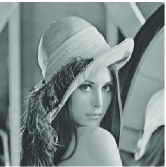
(a) Lena

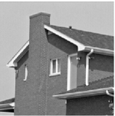
(b) House

(c) Cameraman

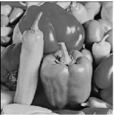
(d) Peppers

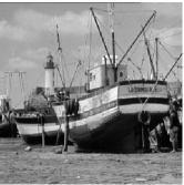
(e) Barchettas

Figure 1: Test images in numerical implementations.

For the sake of simplicity, we use $\sigma$ to denote standard deviation of the white Gaussian noise and $G(hsize,\sigma)$ denotes the symmetric Gaussian low-pass filter of size $hsize$ with standard deviation $\sigma$. In order to compare the visual perception and quality metric point of view, the performance of each method is evaluated in terms of signal to noise ratio ($SNR$) and structural similarity index ($SSIM$): the higher $SNR$ and $SSIM$ the better the restoration results. In addition, we explicitly give the update scheme of the TMM [12] and the FPM [14, 15] as follows

$$\frac{u^{k+1}-u^{k}}{dt}=\left(\lambda K^{T}(Ku^{k}-f)-E_{\alpha}(u^{k})\right)\hskip 10.0pt(\rightarrow TMM)$$ (24)

$$(\lambda K^{T}K+E_{\alpha}(u^{k}))u^{k+1}=\lambda K^{T}f\hskip 45.0pt(\rightarrow FPM)$$ (25)

by choosing a suitable original value $u^{0}$. We set $\alpha=10^{-2}$ for all of numerical implementations. Note the matrix operator in the left of the FPM is symmetric and positive definite. Therefore, we employ the conjugate gradient method to solve it as [14, 15].

We first analyze the performance of our PDM by comparing it with the TMM and FPM for restoration of Lena images with different sizes. Here, the blur and noisy images are corrupted by additive white Gaussian noise with $\sigma=10$ and the Gaussian blur with $G(21,0.6)$. Table 1 illustrates the values of $SNR$, $SSIM$ and CPU time when the numerical algorithms stop. We can observe that $SNR$ and CPU time increases while $SSIM$ decreases when the image size increases. Besides, large parameter $\lambda$ is required to penalize the data fitting term when we increase the size of the test image without increasing the level of noises. From the comparisons of $SNR$, $SSIM$, $Time$ and $Ite$, our PDM is shown better than both the TMM and FPM, especially the CPU time. In fact, the TMM needs more iterations to obtain the steady solution and the FPM needs to solve the linear equation by the numerical methods such as the conjugated gradient method with inner iterations. All of these mean that our proposed PDM is more suitable to deal with the large scale image than the other two methods.

Image	Lena image contaminated by noise with $\sigma=10$.
(S,$\lambda$)	$(128\times 128,0.14)$			$(256\times 256,0.12)$			$(512\times 512,0.11)$
Method	TMM	FPM	PDM	TMM	FPM	PDM	TMM	FPM	PDM
SNR	17.8059	17.7039	18.1492	18.8162	18.7139	19.2730	19.9109	19.8497	20.3225
SSIM	0.8229	0.8397	0.8421	0.7271	0.7272	0.7464	0.6230	0.5907	0.6277
Time(s)	1.6224	4.3056	0.6864	8.1433	23.7746	3.0108	68.6716	126.0488	14.8981
Ite	59	16	32	79	18	36	138	19	38
Image	Lena image contaminated by noise with $\sigma=10$ and Gaussian blur with $G(21.0.6).$
(S,$\lambda$)	$(128\times 128,0.3)$			$(256\times 256,0.25)$			$(512\times 512,0.19)$
Method	TMM	FPM	PDM	TMM	FPM	PDM	TMM	FPM	PDM
SNR	14.8131	15.3534	15.3787	15.6258	16.8751	16.2984	18.2138	18.7663	18.7726
SSIM	0.7568	0.7919	0.7902	0.6160	0.6903	0.6514	0.5595	0.5663	0.5778
Time(s)	1.7784	23.6654	2.6520	4.6020	101.1822	2.6988	56.6596	403.1534	19.9057
Ite	51	29	91	31	30	21	102	24	37

Table 1: The related data by restoring contaminated “Lena” image of different sizes. Here, $\lambda$ and ”Ite” denote the regularization parameter and iteration number, respectively, and ”Time” denotes the CPU time described by second.

Next, we test our PDM on other degraded images, where each test image has its own specialty, i.e., “House” has much more sharp edges, “Cameraman” has more affine regions, and “Peppers” is a relatively smooth image. To generate the degraded images, we add the additive white Gaussian noise and apply the Guassian convolution to the images. Similar results are obtained on these three test images, as shown in Table 2. It is observed that our PDM is more efficient than the other two methods.

Description	Restore noisy images generated by the second row of Figure 1
Image	House			Cameraman			Peppers
$(\sigma,\lambda)$	$(15,0.06)$			$(18,0.06)$			$(20,0.06)$
Method	TMM	FPM	PDM	TMM	FPM	PDM	TMM	FPM	PDM
SNR	18.0276	17.5888	18.1996	16.4785	16.5229	17.1333	15.4266	15.7958	15.7982
SSIM	0.4280	0.3641	0.4117	0.4268	0.4091	0.4383	0.6083	0.6440	0.6333
Time(s)	52.5255	42.4635	6.0060	50.0919	42.5103	5.8812	40.8723	38.7350	5.6160
Ite	500	21	66	500	22	68	415	21	66
Description	Restore noisy and blur images generated by the second row of Figure 1
Image	House			Cameraman			Peppers
$(\sigma,G,\lambda)$	$(15,G(21,0.6),0.07)$			$(18,G(21,0.6),0.08)$			$(20,G(21,0.6),0.07)$
Method	TMM	FPM	PDM	TMM	FPM	PDM	TMM	FPM	PDM
SNR	16.9536	16.5206	16.7436	14.4791	14.2598	14.5334	18.2138	18.7663	18.7726
SSIM	0.3831	0.3309	0.3624	0.3732	0.3597	0.3760	0.5595	0.5663	0.5778
Time(s)	50.9811	93.7410	7.1136	43.8831	97.4850	5.7876	56.6596	403.1534	19.9057
Ite	461	26	66	389	26	54	102	24	37

Table 2: The related data by restoring contaminated image “House”, “Cameraman” and “Peppers”.

Finally, we test our PDM with different smoothing parameters $\alpha$ to validate the effect of $\alpha$ in (15). We use the image “Barchetta”, Figure 1 (e), and generate the degraded images by the white Gaussian noise with $\sigma=10$ and the Gaussian blurring with $G(21,0.6)$. As shown in Table 3, we can obtain the overall best numerical results when $\alpha=0.01$. Furthermore, it is worthy to point out that both the TM and FPM can not be used when the model (15) degenerates to the classic ROF model. We can use the PDM to solve (15) as did in [4] when $\alpha=0$ since the PDM does not depend on the smoothing of the model. By testing our PDM with different $\alpha$, we find that $\alpha=0.01$ is the best choice, which gives comparable or better results than the ROF model.

Description	Barchetta image contaminated by noise with $\sigma=10$
$(\alpha,\lambda)$	(0,0.19)	(0.001,0.18)			(0.01,0.16)			(0.1,0.20)
Method	PDM	TMM	FPM	PDM	TMM	FPM	PDM	TMM	FPM	PDM
SNR	18.6239	17.9886	18.5400	18.6234	18.0055	18.3863	18.6264	18.0459	18.6002	18.6216
SSIM	0.7537	0.7309	0.7540	0.7540	0.7352	0.7503	0.7537	0.7340	0.7543	0.7537
Time(s)	3.1563	29.2344	28.7031	3.1719	20	19.7031	2.4688	8.2188	14.4688	63.6406
Ite	39	232	17	34	135	17	28	52	15	500
Description	Barchetta image contaminated by noise with $\sigma=10$ and Gaussian blurring with $G(21,0.6)$.
$(\alpha,\lambda)$	(0,0.33)	(0.001,0.33)			(0.01,0.33)			(0.1,0.31)
Method	PDM	TMM	FPM	PDM	TMM	FPM	PDM	TMM	FPM	PDM
SNR	15.7181	14.3768	15.7041	15.7188	15.2739	15.7061	15.7186	15.3533	15.7340	15.7039
SSIM	0.6722	0.6126	0.6728	0.6723	0.6520	0.6730	0.6715	0.6588	0.6730	0.6732
Time(s)	11.5938	6.4688	108.1719	11.9063	15.6250	67.4688	8.9219	19.0313	9.1719	58.6406
Ite	103	28	24	104	86	23	75	117	6	500

Table 3: The related data by restoring contaminated “Barchettas” images with different values of $\alpha$.

4 Conclusions

We presented an image restored model based on the minimized surface regularization, which closely relates to the smoothing ROF model [12]. By using the property of conjugate function, we first reformulate the proposed model as a min-max problem and use the primal-dual method [4] to solve the optimization problem. Theoretical convexity conditions guarantee the proposed algorithm converges to a unique global minimizer. Numerical experiments demonstrate that the proposed method holds the potential for efficient and stable computation by compared to the classic time marching method (TMM) [12] and the lagged diffusivity fixed point method (FPM) [14, 15], especially for the large-scale image. In the future, we would like to extend the proposed method to other image processing problem such as image inpainting, reconstruction, registration and also for vector value images, etc.

References

- [1] G. Aubert and P. Kornprobst. Mathematical Problem in Image Processing: partial differential equations and the calculus of variations. Springer, 2008.
- [2] A. Buades, B. Coll, and J.M. Morel. A review of image denoising methods, with a new one. Multiscale Modeling and Simulation, 4(2):490-530, 2006.
- [3] A. Chambolle. An algorithm for total variation minimization and applications. Journal of Mathematical Imaging and Vision, 20(1-2):89-97, 2004.
- [4] A. Chambolle and T. Pock. A first-order primal-dual algorithm for convex problems with applications to imaging. Journal of Mathematical Imaging and Vision, 40(1):120-145, 2011.
- [5] T. Chan and J. Shen. Image Processing and Analysis-Variational, PDE, Wavelet, and Stochastic Methods. SIAM, Philadephia, 2005.
- [6] T. Chan, G. Golub, and P. Mulet. A nonlinear primal-dual method for total variation-based image restoration. SIAM Journal on Scientific Computing, 20(6):1964-1977, 1999.
- [7] I. Ekeland and T. Turbull. Infinite Dimensional Optimization and Convexity. The University of Chicago Press, 1983.
- [8] G Gilboa and S Osher. Nonlocal operators with applications to image processing. Multiscale Modeling and Simulation, 7(3):1005-1028, 2008.
- [9] R. Kimmel, R. Malladi, and N. Sochen. Images as embedded maps and minimal surfaces: movies, color, texture, and volumetric medical images. International Journal of Computer Vision, 39(2): 111-129, 2000.
- [10] O. Scherzer. Handbook of Mathematical Methods in Imaging. Springer New York, 2015.
- [11] N. Sochen, R. Kimmel, and R. Malladi. A general framework for low level vision. IEEE Transactions on Image Processing, 7(3):310-318, 1998.
- [12] L. Rudin, S. Osher, and E. Fatemi. Nolinear total variation based noise removal algorithms. Physica D, 60(1-4):259-268, 1992.
- [13] C. Wu and X. Tai. Augmented Lagrangian method, dual methods, and split Bregman iteration for ROF, vectorial TV, and high order models. SIAM Journal on Imaging Sciences, 3(3):300-339, 2010.
- [14] C. Vogel. Computational Methods for Inverse Problems. SIAM, 2002.
- [15] C. Vogel and M. Oman. Iterative methods for total variation denoising. SIAM Journal on Scientific Computing, 17(1):227-238, 1996.
- [16] D. Zosso and A. Bustin. A primal-dual projected gradient algorithm for efficient Beltrami regularization. UCLA CAM Report 14-52.