Convergence analysis of a locally accelerated preconditioned steepest descent method for Hermitian-definite generalized eigenvalue problems

Abstract

By extending the classical analysis techniques due to Samokish, Faddeev and Faddeeva, and Longsine and McCormick among others, we prove the convergence of preconditioned steepest descent with implicit deflation (PSD-id) method for solving Hermitian-definite generalized eigenvalue problems. Furthermore, we derive a nonasymptotic estimate of the rate of convergence of the PSD-id method. We show that with the proper choice of the shift, the indefinite shift-and-invert preconditioner is a locally accelerated preconditioner, and is asymptotically optimal that leads to superlinear convergence. Numerical examples are presented to verify the theoretical results on the convergence behavior of the PSD-id method for solving ill-conditioned Hermitian-definite generalized eigenvalue problems arising from electronic structure calculations. While rigorous and full-scale convergence proofs of preconditioned block steepest descent methods in practical use still largely eludes us, we believe the theoretical results presented in this paper sheds light on an improved understanding of the convergence behavior of these block methods.

Key words. eigenvalue problem, steepest descent method, preconditioning, superlinear convergence.

MSC. 65F08, 65F15, 65Z05, 15A12.

1 Introduction

We consider the Hermitian-definite generalized eigenvalue problem

$$Hu=\lambda Su,$$ (1.1)

where $H$ and $S$ are $n$-by-$n$ Hermitian matrices and $S$ is positive-definite. The scalar $\lambda$ and nonzero vector $u$ satisfying (1.1) are called eigenvalue and eigenvector, respectively. The pair $(\lambda,u)$ is called an eigenpair. All eigenvalues of (1.1) are known to be real. Our task is to compute few smallest eigenvalues and the corresponding eigenvectors. We are particularly interested in solving the eigenvalue problem (1.1), where the matrices $H$ and $S$ are large and sparse, and there is no obvious gap between the eigenvalues of interest and the rest. Furthermore, $S$ is nearly singular and $H$ and $S$ share a near-nullspace. It is called an ill-conditioned generalized eigenvalue problem in [5], a term we will adopt in this paper. The ill-conditioned generalized eigenvalue problem is considered to be an extremely challenging problem.

Beside examples such as those cited in [5], the ill-conditioned eigenvalue problem (1.1) arises from the discretization of enriched Galerkin methods. The partition-of-unity finite element (PUFE) method [14], which falls within the class of enriched Galerkin methods, is a promising approach in quantum-mechanical materials calculations, see [3] and references therein. In the PUFE method, physics-based basis functions are added to the classical finite element (polynomial basis) approximation, which affords the method improved accuracy at reduced costs versus existing techniques. However, due to near linear-dependence between the polynomial and enriched basis functions, the system matrices that stem from such methods are ill-conditioned, and share a large common near-nullspace. Furthermore, there is in general no clear gap between the eigenvalues that are sought and the rest. Another example of the ill-conditioned eigenvalue problem (1.1) arises from modeling protein dynamics using normal-mode analysis [11, 17, 2, 10].

In this paper, we focus on a preconditioned steepest descent with implicit deflation method, PSD-id method in short, to solve the eigenvalue problems (1.1). The basic idea of the PSD-id method is simple. Denote all the eigenpairs of (1.1) by $(\lambda_{1},u_{1})$, $(\lambda_{2},u_{2})$, …, $(\lambda_{n},u_{n})$, and the eigenvalue and eigenvector matrices by $\Lambda=\operatorname{diag}(\lambda_{1},\lambda_{2},\dots,\lambda_{n})$ and $U=[u_{1}\;u_{2}\;\cdots\;u_{n}]$, respectively. Assume that the eigenvalues $\{\lambda_{i}\}$ are in an ascending order $\lambda_{1}\leq\lambda_{2}\leq\cdots\leq\lambda_{n}$. The following variational principles are well-known, see [27, p.99] for example:

$$\lambda_{i}=\min_{U_{i-1}^{H}Sz=0}\rho(z)\quad\mbox{and}\quad u_{i}=\operatorname*{argmin}_{U_{i-1}^{H}Sz=0}\rho(z),$$ (1.2)

where $U_{i-1}=[u_{1}\;u_{2}\;\cdots\;u_{i-1}]$ and $\rho(z)$ is the Rayleigh quotient

$$\rho(z)=\frac{z^{H}Hz}{z^{H}Sz}.$$ (1.3)

On assuming that $U_{i-1}$ is known, one can find the $i$th eigenpair by minimizing the the Rayleigh quotient $\rho(z)$ with $z$ being $S$-orthogonal against $U_{i-1}$ under the algorithmic framework of the preconditioned steepest descent minimization.

The idea of computing the algebraically largest eigenvalue and its corresponding eigenvector of (1.1) (with $B=I$) using the steepest descent (SD) method dates back to early 1950s [7] and [4, Chap.7]. In [13], block steepest descent (BSD) methods are proposed to compute several eigenpairs simultaneously. The preconditioned steepest descent (PSD) method was introduced around late 1950s [25, 24]. The block PSD (BPSD) methods have appeared in the literature, see [1, 16] and references therein. Like the PSD method, the PSD-id method studied in this paper computes one eigenpair at a time. To compute the $i$th eigenpair, the search subspace of PSD-id is implicitly orthogonalized against the previously computed $i-1$ eigenvectors. Furthermore, the preconditioner at each iteration is flexible (i.e, could change at every iteration) and can be indefinite, instead of being fixed and positive definite as in [25, 1, 16].

Over the past six decades, there has been significant work on the convergence analysis of the SD, PSD and BPSD methods. The convergence of the SD method to compute a single eigenpair is presented in [4, Chap.7]. For the BSD method, the convergence of the first eigenpair is presented in [13] and “ordered convergence” for multiple eigenpairs is declared. The (nonasymptotic) rate of convergence of the PSD method is first studied in [25], which later is proven to be sharp [20]. A comprehensive review of the convergence estimates of the PSD method, is presented in [1]. The theoretical proofs of the convergence of the BPSD method have still largely eluded us, we refer the readers to [1, 19] and two recent papers [15, 16]. In this paper, we present two main results (Theorems 3.1 and 3.2) on the convergence and nonasymptotic rate of convergence of the PSD-id method. These results extend the classical ones due to Faddeev and Faddeeva [4, sec.74] and Samokish [25] for the SD and PSD methods. We show that with the proper choice of the shift, the well-known indefinite shift-and-invert preconditioner is a flexible and locally accelerated preconditioner, and is asymptotically optimal that leads to superlinearly converge of the PSD-id method. Numerical examples shows the superlinear convergence of the PSD-id method with locally accelerated preconditioners for solving ill-conditioned generalized eigenvalue problems (1.1) arising from full self-consistent electronic structure calculations.

We would like to note that the main objective of this paper is to provide a rigorous convergence analysis of the PSD-id method with flexible and locally accelerated preconditioners than to advocate the usage of the PSD-id method in practice. The BPSD methods [1, 16] and a recent proposed locally accelerated BPSD (LABPSD) presented in our previous work [3] have demonstrated their efficiency for finding several eigenpairs simultaneously. While a rigorous and full-scale convergence proof of the the BPSD methods still largely eludes us, we believe the analysis of the PSD-id method presented in this paper can shed light on an improved understanding of the convergence behavior of the BPSD methods such as the LAPBSD method [3] for solving the ill-conditioned generalized eigenvalue problem (1.1) arising from the PUFE simulation of electronic structure calculations.

The rest of this paper is organized as follows. In section 2, we present the PSD-id method and discuss its basic properties. In section 3, we provide a convergence proof and a nonasymptotic estimate of the convergence rate of the PSD-id method. An asymptotically optimal preconditioner is discussed in section 4. Numerical examples to illustrate the theoretical results are presented in section 5. We close with some final remarks in section 6.

In the spirit of reproducible research, Matlab scripts of an implementation of the PSD-id method, and the data that used to generate numerical results presented in this paper can be obtained from the URL http://dsec.pku.edu.cn/$\sim$yfcai/psdid.html.

2 Algorithm

Assuming that $U_{i-1}$ is already known, by (1.2), one can find the $i$th eigenpair by minimizing the Rayleigh quotient $\rho(z)$ with $z$ being $S$-orthogonal against $U_{i-1}$. Specifically, let us denote by $(\lambda_{i;j},u_{i;j})$ the $j$th approximation of $(\lambda_{i},u_{i})$ and assume that

$$U^{H}_{i-1}Su_{i;j}=0,\quad\|u_{i;j}\|_{S}=1\quad\mbox{and}\quad\lambda_{i;j}=\rho(u_{i;j}).$$ (2.1)

To compute the $(j+1)$st approximate eigenpair $(\lambda_{i;j+1},u_{i;j+1})$, by the steepest descent approach, the steepest decreasing direction of $\rho(z)$ is opposite to the gradient of $\rho(z)$ at $z=u_{i;j}$:

$$\nabla\rho(u_{i;j})=2(H-\lambda_{i;j}S)u_{i;j}=2r_{i;j}.$$

Furthermore, to accelerate the convergence, we use the following preconditioned search vector

$$p_{i;j}=-K_{i;j}r_{i;j},$$ (2.2)

where $K_{i;j}$ is a preconditioner. By a Rayleigh-Ritz projection based implementation, the $(j+1)$st approximate eigenpair $(\lambda_{i;j+1},u_{i;j+1})$ computed by the preconditioned steepest descent method is given by

$$(\lambda_{i;j+1},u_{i;j+1})=(\gamma_{i},Z_{j}w_{i}),$$ (2.3)

where $(\gamma_{i},w_{i})$ is the $i$th eigenpair of the projected matrix pair $(H_{R},S_{R})=(Z^{H}_{j}HZ_{j},Z^{H}_{j}SZ_{j})$, $\|w_{i}\|_{S_{R}}=1$, and $Z_{j}=[U_{i-1}\;u_{i;j}\;p_{i;j}]$ is the basis matrix of the projection subspace. Here we assume that $Z_{j}$ is of full column rank.

Algorithm 1 is a summary of the aforementioned procedure. Since the first eigenvectors $U_{i-1}$ are implicitly deflated in the Rayleigh-Ritz procedure, we call Algorithm 1 a preconditioned steepest descent with implicit deflation, PSD-id in short. We note that the preconditioner $K_{i;j}$ is flexible. It can be changed at each iteration. If the preconditioner is fixed as a uniform positive definite matrix, i.e., $K_{i;j}=K>0$, then Algorithm 1 is the SIRQIT-G2 algorithm in [13] with $K=I$ and initial vectors $X^{(0)}=[U_{i-1}\,u_{i;0}]$, and is the BPSD method [9] with initial vectors $[U_{i-1}\,u_{i;0}]$.

Algorithm 1 PSD-id

0:  $U_{i-1}$ and initial vector $u_{i;0}$

0:  Approximate eigenpair $(\lambda_{i},u_{i})$ of $(\lambda_{i},u_{i})$

1:  $\lambda_{i;0}=\rho(u_{i;0})$

2:  for $j=0,1,\ldots$, until convergence do

3:     compute $r_{i;j}=Hu_{i;j}-\lambda_{i;j}Su_{i;j}$

4:     precondition $p_{i;j}=-K_{i;j}r_{i;j}$

5:     compute the $i$th eigenpair $(\gamma_{i},w_{i})$ of $(H_{R},S_{R})=(Z^{H}_{j}HZ_{j},Z^{H}_{j}SZ_{j})$, $Z_{j}=[U_{i-1}\;u_{i;j}\;p_{i;j}]$

6:     update $\lambda_{i;j+1}=\gamma_{i}$ and $u_{i;j+1}=Z_{j}w_{i}$

7:  end for

If Algorithm 1 does not breakdown, i.e., the matrices $Z_{j}$ on line 5 are full column rank for all $j$, then a sequence of approximate eigenpairs $\{(\lambda_{i;j},u_{i;j})\}_{j}$ are produced. The following proposition gives basic properties of the sequence. In particular, if the initial vector $u_{i;0}$ does not satisfy the assumption (2.1), the first approximate vector $u_{i;1}$ computed by Algorithm 1 will suffice.

Proposition 2.1.

If $Z_{j}$ is of full column rank, then

• $U^{H}_{i-1}Su_{i;j+1}=0$.

• $\|u_{i;j+1}\|_{S}=1$.

• $\lambda_{i;j+1}\geq\lambda_{i}$.

• $\lambda_{i;j+1}\leq\lambda_{i;j}$.

Proof.

Results (a) and (b) are verified by straightforward calculation. The result (c) follows from the inequality

$$\lambda_{i;j+1}=\rho({u}_{i;j+1})\geq\min_{U_{i-1}^{H}Sz=0}\rho(z)=\lambda_{i}.$$

Finally, the result (d) follows from the facts that

$$\lambda_{i;j+1}=\lambda_{i}(H_{R},S_{R})=\min_{U_{i-1}^{H}SZ_{j}w=0}\rho(Z_{j}w)\leq\rho(Z_{j}w)|_{w=e_{i}}=\rho(u_{i;j})=\lambda_{i;j},$$

where $e_{i}$ is the $i$th column vector of identity matrix of order $i+1$. ∎

The following proposition shows that with the proper choice of the preconditioner $K_{i;j}$, the basis matrix $Z_{j}=[U_{i-1}\;u_{i;j}\;p_{i;j}]$ is of full column rank, which implies that Algorithm 1 does not breakdown.

Proposition 2.2.

If $r_{i;j}\neq 0$ and $K_{i;j}$ is chosen such that

$$K^{c}_{i;j}:=(U_{i-1}^{c})^{H}SK_{i;j}SU_{i-1}^{c}>0,$$ (2.4)

then the basis matrix $Z_{j}$ is of full column rank. Here $U_{i-1}^{c}$ is complementary eigenvector matrix of $U_{i-1}$, i.e., $U_{i-1}^{c}=[u_{i}\;\cdots\;u_{n}]$.

Proof.

We prove that $Z_{j}$ is of full column rank by showing that

$$\det(H_{R}-\lambda_{i;j}S_{R})=\det(Z^{H}_{j}(H-\lambda_{i;j}S)Z_{j})\neq 0.$$

First, it can be verified that the projected matrix pair $(H_{R},S_{R})$ can be factorized as follows:

$$(H_{R},S_{R})=L^{-1}\left(\begin{bmatrix}\Lambda_{i-1}&0\\ 0&H_{\bot}\end{bmatrix},\begin{bmatrix}I_{i-1}&0\\ 0&S_{\bot}\end{bmatrix}\right)L^{-H},$$ (2.5)

where

$$L=\begin{bmatrix}I_{i-1}&0&0\\ 0&1&0\\ -p_{i;j}^{H}SU_{i-1}&0&1\end{bmatrix},\quad H_{\bot}=Z_{\bot}^{H}HZ_{\bot},\quad S_{\bot}=Z_{\bot}^{H}SZ_{\bot},$$

and $Z_{\bot}=[u_{i;j}\;p_{\bot}]$ and $p_{\bot}=U_{i-1}^{c}(U_{i-1}^{c})^{H}Sp_{i;j}$. Consequently, we have

$$\det(H_{R}-\lambda_{i;j}S_{R})=\det(\Lambda_{i-1}-\lambda_{i;j}I)\det(H_{\bot}-\lambda_{i;j}S_{\bot}).$$ (2.6)

By Proposition 2.1(c), we have $\lambda_{i;j}\geq\lambda_{i}$. Since $r_{i;j}\neq 0$, $\lambda_{i;j}>\lambda_{i}$. Hence, we conclude that

$$\det(\Lambda_{i-1}-\lambda_{i;j}I)\neq 0.$$ (2.7)

Next we show that $\det(H_{\bot}-\lambda_{i;j}S_{\bot})\neq 0$. We first note that since $U_{i-1}^{H}Su_{i;j}=0$, there exists a vector $a$ such that $u_{i;j}=U_{i-1}^{c}a$. Then it follows that

$$r_{i;j}=(H-\lambda_{i;j}S)U_{i-1}^{c}a=SU_{i-1}^{c}(\Lambda_{i-1}^{c}-\lambda_{i;j}I)a=SU_{i-1}^{c}(U_{i-1}^{c})^{H}r_{i;j},$$ (2.8)

where $\Lambda_{i-1}^{c}=\operatorname{diag}(\lambda_{i},\ldots,\lambda_{n})$. Note that $(U_{i-1}^{c})^{H}r_{i;j}\neq 0$ since $r_{i;j}\neq 0$. Furthermore, using (2.8) and (2.4), we have

$$\det(H_{\bot}-\lambda_{i;j}S_{\bot}) =\det\begin{bmatrix}0&r_{i;j}^{H}p_{\bot}\\ p_{\bot}^{H}r_{i;j}&p_{\bot}^{H}(H-\lambda_{i;j}S)p_{\bot}\end{bmatrix}$$

$$=-|p_{\bot}^{H}r_{i;j}|^{2}$$

$$=-|r_{i;j}^{H}U_{i-1}^{c}(U_{i-1}^{c})^{H}SK_{i;j}SU_{i-1}^{c}(U_{i-1}^{c})^{H}r_{i;j}|^{2}$$

$$=-|r_{i;j}^{H}U_{i-1}^{c}{K}^{c}_{i;j}(U_{i-1}^{c})^{H}r_{i;j}|<0.$$ (2.9)

By (2.6), (2.7) and (2.9), we conclude that $H_{R}-\lambda_{i;j}S_{R}$ is nonsingular, which implies that $Z_{j}$ is of full column rank. ∎

Definition 2.1.

A preconditioner $K_{i;j}$ satisfying the condition (2.4) is called an effectively positive definite preconditioner.

We note that an effectively positive definite preconditioner $K_{i;j}$ with $i>1$ is not necessarily to be symmetric positive definite. For example, for any $\lambda_{1}<\sigma<\lambda_{i}$ and $\sigma$ is not an eigenvalue of $(H,S)$, $K_{i;j}=(H-\sigma S)^{-1}$ is effectively positive definite, although $K_{i;j}$ is indefinite.

If the preconditioner $K_{i;j}$ is chosen such that the search vector $p_{i;j}=-K_{i;j}r_{i;j}$ satisfies

$$U^{H}S({u}_{i;j}+p_{i;j})=\xi=(\xi_{1},\xi_{2},\dots,\xi_{n})^{H}\quad\mbox{with $\xi_{i}\neq 0$ and $\xi_{j}=0$ for $j>i$},$$ (2.10)

then

$$\lambda_{i;j+1} =\min_{U_{i-1}^{H}SZ_{j}w=0}\rho(Z_{j}w)$$

$$=\min_{w}\rho(U_{i-1}^{c}(U_{i-1}^{c})^{H}SZ_{j}w)$$

$$=\min_{v}\rho(U_{i-1}^{c}(U_{i-1}^{c})^{H}S[u_{i;j}\ p_{i;j}]v)$$

$$\leq\rho(U_{i-1}^{c}(U_{i-1}^{c})^{H}S[u_{i;j}\ p_{i;j}]v)|_{v=[1\;1]^{\top}}$$

$$=\rho(U_{i-1}^{c}(U_{i-1}^{c})^{H}S(u_{i;j}+p_{i;j}))$$

$$=\rho(U_{i-1}^{c}(U_{i-1}^{c})^{H}SU\xi)$$

$$=\rho(\xi_{i}u_{i})=\lambda_{i}.$$ (2.11)

Therefore, combining the inequality (2.11) and Proposition 2.1(c), we have $\lambda_{i;j+1}=\lambda_{i}$. In this case, we refer to $p_{i;j}$ satisfying the equation (2.10) as an ideal search direction. The notion of an ideal search direction not only helps assessing the quality of a preconditioned search direction, but also tells the desired property for the solution of the preconditioning equation $p_{i;j}=-K_{i;j}r_{i;j}$.

3 Convergence analysis

In this section, we prove the convergence of the PSD-id method and derive a nonasymptotic estimate of the convergence rate. For brevity, we assume that for the desired $i$th eigenvalue $\lambda_{i}$, it satisfies $\lambda_{i-1}<\lambda_{i}<\lambda_{i+1}$. Otherwise by replacing $\lambda_{i+1}$ by the smallest eigenvalue of $(H,S)$ which is larger than $\lambda_{i}$, all results in this section still hold, the proofs are similar.

3.1 Convergence results

Assume that the preconditioner $K_{i;j}$ is effectively positive definite, then by Proposition 2.1(d) and (2.9), we have that $\lambda_{i;j+1}$ is strictly less than $\lambda_{i;j}$,

$$\lambda_{i;j+1}<\lambda_{i;j}.$$ (3.1)

Furthermore, by Proposition 2.1(c) and (3.1), the approximate eigenvalue sequence $\{\lambda_{i;j}\}_{j}$ is a monotonically decreasing and is bounded below by $\lambda_{i}$, i.e.,

$$\lambda_{i;0}>\lambda_{i;1}>\cdots>\lambda_{i;j}>\lambda_{i;j+1}>\dots\geq\lambda_{i}.$$ (3.2)

Therefore, the sequence $\{\lambda_{i;j}\}_{j}$ must converge. Does it converge to the $i$th eigenvalue $\lambda_{i}$ of $(H,S)$? How about the corresponding $\{u_{i;j}\}_{j}$? We will answer these questions in this subsection. First, we give the following lemma to quantify the difference between two consecutive approximates $\lambda_{i;j}$ and $\lambda_{i;j+1}$ of $\lambda_{i}$.

Lemma 3.1.

If $r_{i;j}\neq 0$ and the preconditioner $K_{i;j}$ is effectively positive definite, then

$$\lambda_{i;j}-\lambda_{i;j+1}\geq\sqrt{g^{2}+\phi^{2}}-g,$$ (3.3)

where $g=(\lambda_{n}-\lambda_{i})/2$ and $\phi={\|r_{i;j}\|_{S^{-1}}}/{\kappa(K^{c}_{i;j})}$, $\kappa(K^{c}_{i;j})$ is the condition number of ${K}^{c}_{i;j}$ defined in (2.4).

Proof.

Let $H_{\bot}$ and $S_{\bot}$ be the matrices defined in (2.5). By $S$-orthogonalizing $p_{i;j}$ against $[U_{i-1}\;u_{i;j}]$, the resulting vector $\hat{p}=(I-u_{i;j}u_{i;j}^{H}S)P_{i-1}p_{i;j}$ must be nonzero since $Z_{j}=[U_{i-1}\;u_{i;j}\;p_{i;j}]$ is of full column rank (Lemma 2.2). Therefore, it holds that $\hat{p}^{H}S\hat{p}>0$. By straightforward calculations, we have

$$\det(H_{\bot}-\mu S_{\bot}) =\det\left(\begin{bmatrix}\lambda_{i;j}&u_{i;j}^{H}H\hat{p}\\ \hat{p}^{H}Hu_{i;j}&\hat{p}^{H}H\hat{p}\end{bmatrix}-\mu\begin{bmatrix}1&0\\ 0&\hat{p}^{H}S\hat{p}\end{bmatrix}\right)$$

$$=\hat{p}^{H}S\hat{p}(\lambda_{i;j}-\mu)(\rho(\hat{p})-\mu)-|u_{i;j}^{H}H\hat{p}|^{2}$$

$$=\hat{p}^{H}S\hat{p}\left[(\lambda_{i;j}-\mu)^{2}+(\rho(\hat{p})-\lambda_{i;j})(\lambda_{i;j}-\mu)-\frac{|u_{i;j}^{H}H\hat{p}|^{2}}{\hat{p}^{H}S\hat{p}}\right].$$ (3.4)

By the definition of $\lambda_{i;j+1}$ in (2.3), the identity (2.6), we know that $\lambda_{i;j+1}$ is the smaller root of the quadratic polynomial (3.4) of $\mu$. In addition, by (3.2), we know that $\lambda_{i;j}-\lambda_{i;j+1}$ is positive. Therefore $\lambda_{i;j}-\lambda_{i;j+1}$ is the positive root of the following quadratic equation in $t$:

$$t^{2}+(\rho(\hat{p})-\lambda_{i;j})t-\frac{|u_{i;j}^{H}H\hat{p}|^{2}}{\hat{p}^{H}S\hat{p}}=0.$$

Then it follows that

$$\lambda_{i;j}-\lambda_{i;j+1}=-\frac{\rho(\hat{p})-\lambda_{i;j}}{2}+\sqrt{\left(\frac{\rho(\hat{p})-\lambda_{i;j}}{2}\right)^{2}+\frac{|u_{i;j}^{H}H\hat{p}|^{2}}{\hat{p}^{H}S\hat{p}}}.$$ (3.5)

In what follows, we give the estimates of the quantities $|\rho(\hat{p})-\lambda_{i;j}|$, $|u_{i;j}^{H}H\hat{p}|^{2}$ and $\hat{p}^{H}S\hat{p}$, respectively.

For the quantity $|\rho(\hat{p})-\lambda_{i;j}|$, using the fact that for any nonzero $z$ satisfying $U_{i-1}^{H}Sz=0$, it holds $\lambda_{i}\leq\rho(z)\leq\lambda_{n}$, then using $U_{i-1}^{H}S\hat{p}=0$ and $U_{i-1}^{H}Su_{i;j}=0$, we have

$$0\leq|\rho(\hat{p})-\lambda_{i;j}|\leq\lambda_{n}-\lambda_{i}=2g.$$ (3.6)

For the quantity $|u_{i;j}^{H}H\hat{p}|^{2}$, we have

$$|u_{i;j}^{H}H\hat{p}| =|u_{i;j}^{H}H(I-u_{i;j}u_{i;j}^{H}S)U_{i-1}^{c}(U_{i-1}^{c})^{H}SK_{i;j}r_{i;j}|$$ (3.7a)

$$=|\big{[}u_{i;j}^{H}H-\lambda_{i;j}u_{i;j}^{H}S\big{]}U_{i-1}^{c}\big{[}(U_{i-1}^{c})^{H}SK_{i;j}SU_{i-1}^{c}\big{]}(U_{i-1}^{c})^{H}r_{i;j}|$$ (3.7b)

$$=|r_{i;j}^{H}U_{i-1}^{c}K^{c}_{i;j}(U_{i-1}^{c})^{H}r_{i;j}|$$ (3.7c)

$$\geq\lambda_{\min}(K^{c}_{i;j})\|(U_{i-1}^{c})^{H}r_{i;j}\|^{2}$$ (3.7d)

$$=\lambda_{\min}(K^{c}_{i;j})\|r_{i;j}\|_{S^{-1}}^{2},$$ (3.7e)

where (3.7a) uses the definition of $\hat{p}$ and (2.2), (3.7b) uses the fact that $r_{i;j}=SU_{i-1}^{c}(U_{i-1}^{c})^{H}r_{i;j}$, (3.7c) and (3.7d) use the definition of $K^{c}_{i;j}$ in (2.4) and the assumption that $K^{c}_{i;j}$ is symmetric positive definite, and (3.7e) is based on the following calculations:

$$\|(U_{i-1}^{c})^{H}r_{i;j}\|^{2} =r_{i;j}^{H}U_{i-1}^{c}(U_{i-1}^{c})^{H}r_{i;j}$$

$$=r_{i;j}^{H}U_{i-1}^{c}(U_{i-1}^{c})^{H}r_{i;j}+r_{i;j}^{H}U_{i-1}U_{i-1}^{H}r_{i;j} (U_{i-1}^{H}r_{i;j}=0)$$

$$=r_{i;j}^{H}UU^{H}r_{i;j}$$

$$=r_{i;j}^{H}S^{-1}r_{i;j} (UU^{H}=S^{-1})$$

$$=\|r_{i;j}\|_{S^{-1}}^{2}.$$

For the quantity $\hat{p}^{H}S\hat{p}$, we have

$$\hat{p}^{H}S\hat{p} =(r_{i;j})^{H}K_{i;j}SU_{i-1}^{c}\big{[}(U_{i-1}^{c})^{H}(I-Su_{i;j}u_{i;j}^{H})S(I-u_{i;j}u_{i;j}^{H}S)U_{i-1}^{c}\big{]}(U_{i-1}^{c})^{H}SK_{i;j}r_{i;j}$$

$$\leq\|(U_{i-1}^{c})^{H}(I-Su_{i;j}u_{i;j}^{H})S(I-u_{i;j}u_{i;j}^{H}S)U_{i-1}^{c}\|\|(U_{i-1}^{c})^{H}SK_{i;j}r_{i;j}\|^{2}$$

$$\leq\|(U_{i-1}^{c})^{H}SK_{i;j}r_{i;j}\|^{2}$$

$$=\|K^{c}_{i;j}(U_{i}^{c})^{H}r_{i;j}\|^{2}$$

$$\leq\lambda_{\max}(K^{c}_{i;j})^{2}\|(U_{i-1}^{c})^{H}r_{i;j}\|^{2}$$

$$=\lambda_{\max}(K^{c}_{i;j})^{2}\|r_{i;j}\|_{S^{-1}}^{2},$$ (3.8)

where the second inequality use the fact that

$$\| (U_{i-1}^{c})^{H}(I-Su_{i;j}u_{i;j}^{H})S(I-u_{i;j}u_{i;j}^{H}S)U_{i-1}^{c}\|$$

$$=\| (U_{i-1}^{c})^{H}S^{{\frac{1}{2}}}(I-S^{\frac{1}{2}}u_{i;j}u_{i;j}^{H}S^{\frac{1}{2}})(I-S^{\frac{1}{2}}u_{i;j}u_{i;j}^{H}S^{\frac{1}{2}})S^{\frac{1}{2}}U_{i-1}^{c}\|$$

$$\leq\| (I-S^{\frac{1}{2}}u_{i;j}u_{i;j}^{H}S^{\frac{1}{2}})\|^{2}\|S^{\frac{1}{2}}U_{i-1}^{c}\|^{2}\leq 1.$$

Finally, by (3.6), (3.7e) and (3.8), it follows from (3.5) that

$$\lambda_{i;j}-\lambda_{i;j+1}\geq -\frac{|\rho(\hat{p})-\lambda_{i;j}|}{2}+\sqrt{\bigg{(}\frac{\rho(\hat{p})-\lambda_{i;j}}{2}\bigg{)}^{2}+\frac{|u_{i;j}^{H}H\hat{p}|^{2}}{\hat{p}^{H}S\hat{p}}}$$

$$\geq -\frac{\lambda_{n}-\lambda_{i}}{2}+\sqrt{\bigg{(}\frac{\lambda_{n}-\lambda_{i}}{2}\bigg{)}^{2}+\frac{\|r_{i;j}\|^{2}_{S^{-1}}}{\kappa^{2}(K^{c}_{i;j})}}$$

$$= -g+\sqrt{g^{2}+\phi^{2}}.$$

This completes the proof. ∎

We note that in [4, Chap.7], for the steepest descent method to compute the largest eigenvalue $\lambda_{n}$ of a Hermitian matrix, it shows that

$$\lambda_{n;j+1}-\lambda_{n;j}\geq\frac{\|r_{n;j}\|^{2}}{\lambda_{n}-\lambda_{1}}.$$

Then it is established that $\lambda_{n;j}$ converges to $\lambda_{n}$, and $u_{n;j}$ converges to $u_{n}$ directionally. Lemma 3.1 and the following theorem are generalizations that are not limited to the largest eigenpair, and include the usage of flexible preconditioners.

Theorem 3.1.

If the initial estimate eigenvalue $\lambda_{i;0}$ satisfying $\lambda_{i}<\lambda_{i;0}<\lambda_{i+1}$, and the flexible preconditioners $K_{i;j}$ are an effectively positive definite for all $j$ and $\mbox{sup}_{j}\kappa(K^{c}_{i;j})=q<\infty$, then the sequence $\{(\lambda_{i;j},u_{i;j})\}_{j}$ generated by the PSD-id method converges to the desired pair $(\lambda_{i},u_{i})$, i.e.,

• $\lim_{j\rightarrow\infty}\lambda_{i;j}=\lambda_{i}$.

• $\lim_{j\rightarrow\infty}\|r_{i;j}\|_{S^{-1}}=0$, namely $u_{i;j}$ converges to $u_{i}$ directionally.

Proof.

To prove (a), we first notice that $\{\lambda_{i;j}\}_{j}$ is a monotonic decreasing sequence, and is bounded by $\lambda_{i}$ from below. So there exists a real number $\tilde{\lambda}_{i}$ such that $\lambda_{i;j}\rightarrow\tilde{\lambda}_{i}$ as $j\rightarrow\infty$. Now we show by contradiction that $\tilde{\lambda}_{i}=\lambda_{i}$. For any $u_{i;j}$ ($\|u_{i;j}\|_{S}=1$), we have

$$\|r_{i;j}\|_{S^{-1}} =\|(H-\lambda_{i;j}S)u_{i;j}\|_{S^{-1}}$$

$$\geq\|(H-\tilde{\lambda}_{i}S)u_{i;j}\|_{S^{-1}}-(\lambda_{i;j}-\tilde{\lambda}_{i})\|Su_{i;j}\|_{S^{-1}}$$

$$\geq\min_{k}{|\lambda_{k}-\tilde{\lambda}_{i}|}-(\lambda_{i;j}-\tilde{\lambda}_{i}).$$

As $\lim_{j\rightarrow\infty}\lambda_{i;j}=\tilde{\lambda}_{i}$, there exists a $j_{0}$ such that for any $j\geq j_{0}$,

$$\|r_{i;j}\|_{S^{-1}}>{\frac{1}{2}}\min_{k}|\lambda_{k}-\tilde{\lambda}_{i}|.$$

By defining $d(r,\kappa):=-g+\sqrt{g^{2}+(r/\kappa)^{2}}$, it follows from Lemma 3.1 that for any $j\geq j_{0}$, it holds that

$$\lambda_{i;j}-\lambda_{i;j+1}\geq d(\|r_{i;j}\|_{S^{-1}},\kappa_{i;j})>d(\min_{k}|\lambda_{k}-\tilde{\lambda}_{i}|/2,\kappa_{i;j})\geq d(\min_{k}|\lambda_{k}-\tilde{\lambda}_{i}|/2,q),$$

which in the limit becomes

$$0>d(\min_{k}|\lambda_{k}-\tilde{\lambda}_{i}|/2,q).$$

This is a contradiction to the fact that $d(\min_{k}|\lambda_{k}-\tilde{\lambda}_{i}|/2,q)$ is a positive constant.

To prove (b), by using $\lim_{j\rightarrow\infty}\lambda_{i;j}=\lambda_{i}$ and Lemma 3.1, we have

$$\lim_{j\rightarrow\infty}d(\|r_{i;j}\|_{S^{-1}},q)\leq\lim_{j\rightarrow\infty}d(\|r_{i;j}\|_{S^{-1}},\kappa_{i;j})\leq\lim_{j\rightarrow\infty}(\lambda_{i;j}-\lambda_{i;j+1})=0.$$

Consequently, $\lim_{j\rightarrow\infty}d(\|r_{i;j}\|_{S^{-1}},q)=0$, which leads to $\lim_{j\rightarrow\infty}\|r_{i;j}\|_{S^{-1}}=0$ since $1\leq q<\infty$. ∎

We note that in Theorem 3.1, without assuming $\lambda_{i;0}<\lambda_{i+1}$, by similar argument, we can conclude $\{\lambda_{i;j}\}_{j}$ converges to an eigenvalue $\lambda_{k}$ for some $k\geq i$, and $\{u_{i;j}\}_{j}$ directionally converges to the corresponding eigenvector $u_{k}$.

3.2 Rate of convergence

Theorem 3.1 concludes the convergence of the sequence $\{\lambda_{i;j}\}_{j}$, what follows we derive a nonasymptotic estimate of the convergence rate of $\{\lambda_{i;j}\}_{j}$ based on the work of Samokish in 1958 [25]. We begin by recalling the following equalities for the projection matrix $P_{i-1}=I-U_{i-1}U^{H}_{i-1}S={U}_{i-1}^{c}({U}_{i-1}^{c})^{H}S$:

$$P_{i-1}u_{i;j} =u_{i;j},$$ (3.9a)

$$P_{i-1}^{2} =P_{i-1},$$ (3.9b)

$$P_{i-1}^{H}(H-\lambda_{i}S) =(H-\lambda_{i}S)P_{i-1},$$ (3.9c)

$$P_{i-1}^{H}S =SP_{i-1},$$ (3.9d)

First, we have the following lemma.

Lemma 3.2.

Define

$$M=P_{i-1}^{H}(H-\lambda_{i}S)P_{i-1}$$ (3.10)

and assume that $K_{i;j}$ is effectively positive definite.

• $M$ is positive semi-definite and $M=GG^{H}$, where $G=S{U}_{i}^{c}({\Lambda}_{i}^{c}-\lambda_{i}I)^{{\frac{1}{2}}}$ is of full column rank.

• All eigenvalues of $G^{H}K_{i;j}G$ are positive.

• The eigenvalues of $K_{i;j}M$ are given by

  $$\lambda(K_{i;j}M)=\{0_{[i]}\}\cup\lambda\big{(}G^{H}K_{i;j}G\big{)},$$ (3.11)

  where $0_{[i]}$ stands for the multiplicity $i$ of the number 0.

Proof.

(a) By the definitions of $M$ and $P_{i-1}$, it easy to see that

$$M =S{U}_{i-1}^{c}({U}_{i-1}^{c})^{H}(H-\lambda_{i}S){U}_{i-1}^{c}({U}_{i-1}^{c})^{H}S$$

$$=S{U}_{i}^{c}({\Lambda}_{i}^{c}-\lambda_{i}I)({U}_{i}^{c})^{H}S=GG^{H}\geq 0,$$

where $G=S{U}_{i}^{c}({\Lambda}_{i}^{c}-\lambda_{i}I)^{{\frac{1}{2}}}$.

(b) Direct calculation leads to

$$G^{H}K_{i;j}G=({\Lambda}_{i}^{c}-\lambda_{i}I)^{{\frac{1}{2}}}\widetilde{K}_{22}({\Lambda}_{i}^{c}-\lambda_{i}I)^{{\frac{1}{2}}},$$

where $\widetilde{K}_{22}$ is the trailing $(n-i)$-by-$(n-i)$ principal submatrix of $K^{c}_{i;j}$ by deleting its first $i-1$ rows and first $i-1$ columns. Since $K_{i;j}$ is effectively positive definite, we know that $K^{c}_{i;j}>0$ and hence $\widetilde{K}_{22}>0$. Thus all eigenvalues of $G^{H}K_{i;j}G$ are positive.

(c) It follows that

$$\lambda(K_{i;j}M)=\lambda(K_{i;j}GG^{H})=\{0_{[i]}\}\cup\lambda(G^{H}K_{i;j}G),$$

where we use the well-known identity $\lambda(AB)=\{0_{[m-n]}\}\cup\lambda(BA)$ for $A\in\mathbb{C}^{m\times n}$ and $B\in\mathbb{C}^{n\times m}$ and $m\geq n$. ∎

We now give a nonasymptotic estimate of the convergence rate of PSD-id (Algorithm 1).

Theorem 3.2.

Let $\epsilon_{i;j}=\lambda_{i;j}-\lambda_{i}$ and $\lambda_{i;j}$ be localized, namely

$$\tau(\sqrt{\theta_{i;j}\epsilon_{i;j}}+\delta_{i;j}\epsilon_{i;j})<1,$$ (3.12)

then

$$\epsilon_{i;j+1}\leq\Bigg{[}\frac{\Delta+\tau\sqrt{\theta_{i;j}\epsilon_{i;j}}}{1-\tau(\sqrt{\theta_{i;j}\epsilon_{i;j}}+\delta_{i;j}\epsilon_{i;j})}\Bigg{]}^{2}\epsilon_{i;j},$$ (3.13)

where $\theta_{i;j}=\|S^{{\frac{1}{2}}}K_{i;j}MK_{i;j}S^{{\frac{1}{2}}}\|$, $\delta_{i;j}=\|S^{{\frac{1}{2}}}K_{i;j}S^{{\frac{1}{2}}}\|$, $\Delta={(\Gamma-\gamma)}/{(\Gamma+\gamma)}$, $\Gamma$ and $\gamma$ are the largest and smallest positive eigenvalues of $K_{i;j}M$, respectively, and $\tau={2}/{(\Gamma+\gamma)}$.

Proof.

Recall $Z_{\bot}=[\,u_{i;j}\;P_{i-1}p_{i;j}\,]$ defined in (2.5). It is easy to see that by using $Z_{\bot}$, the $(j+1)$th approximate eigenpair $(\lambda_{i;j+1},u_{i;j})$ can be written as

$$\lambda_{i;j+1}=\min_{v}\rho(Z_{\bot}v).$$

Considering a choice of the vector $v$ for the line search, we have

$$\lambda_{i;j+1}=\min_{v}\rho(Z_{\bot}v)\leq\rho(Z_{\bot}v)|_{v=[1\;\tau]^{\top}}=\rho(z),$$

where $z=Z_{\bot}[1\;\tau]^{\top}=u_{i;j}+\tau P_{i-1}p_{i;j}$. Consequently, we have

$$\epsilon_{i;j+1}=\lambda_{i;j+1}-\lambda_{i}\leq\rho(z)-\lambda_{i}=\frac{z^{H}(H-\lambda_{i}S)z}{z^{H}Sz}.$$ (3.14)

In the following, we provide estimates for the numerator and denominator of the upper bound (3.14).

For the numerator of the upper bound in (3.14), it follows that

$$z^{H}(H-\lambda_{i}S)z =(u_{i;j}+\tau p_{i;j})^{H}P_{i-1}^{H}(H-\lambda_{i}S)P_{i-1}(u_{i;j}+\tau p_{i;j})$$

$$=\|u_{i;j}+\tau p_{i;j}\|^{2}_{M}$$

$$=\|u_{i;j}-\tau P_{i-1}K_{i;j}(H-\lambda_{i;j}S)u_{i;j}\|_{M}^{2}$$

$$=\|u_{i;j}-\tau P_{i-1}K_{i;j}[(H-\lambda_{i}S)-\epsilon_{i;j}S]u_{i;j}\|_{M}^{2}$$

$$=\|[I-\tau P_{i-1}K_{i;j}(H-\lambda_{i}S)]u_{i;j}+\tau\epsilon_{i;j}P_{i-1}K_{i;j}Su_{i;j}\|_{M}^{2}$$

$$=\|[I-\tau P_{i-1}K_{i;j}P_{i-1}^{H}(H-\lambda_{i}S)P_{i-1}]u_{i;j}+\tau\epsilon_{i;j}P_{i-1}K_{i;j}Su_{i;j}\|_{M}^{2}$$ (3.15a)

$$\leq\big{(}\|[I-\tau P_{i-1}K_{i;j}M]u_{i;j}\|_{M}+\tau\epsilon_{i;j}\|P_{i-1}K_{i;j}Su_{i;j}\|_{M}\big{)}^{2},$$ (3.15b)

where the equality (3.15a) uses the identities (3.9a) and (3.9c). The inequality (3.15b) uses the triangular inequality of the vector norm induced by the semi-positive definite matrix $M$. For the first term in (3.15b), using $M=GG^{H}$ and $G^{H}P_{i-1}=G^{H}$, where $G$ is defined in Lemma 3.2, we have

$$\|[I-\tau P_{i-1}K_{i;j}M]u_{i;j}\|_{M} =\|G^{H}[I-\tau P_{i-1}K_{i;j}GG^{H}]u_{i;j}\|$$

$$=\|(I-\tau G^{H}K_{i;j}G)(G^{H}u_{i;j})\|$$

$$\leq\|(I-\tau G^{H}K_{i;j}G)\|\|u_{i;j}\|_{M}.$$ (3.16)

Note that by Lemma 3.2, it yields that

$$\|(I-\tau G^{H}K_{i;j}G)\| =\max_{k}|1-\tau\lambda_{k}(G^{H}K_{i;j}G)|$$

$$=\max\{|1-\tau\gamma|,|1-\tau\Gamma|\}$$

$$=\frac{\Gamma-\gamma}{\Gamma+\gamma}=\Delta.$$ (3.17)

Consequently, we can rewrite (3.16) as

$$\|[I-\tau P_{i-1}K_{i;j}M]u_{i;j}\|_{M}\leq\Delta\,\|u_{i;j}\|_{M}=\Delta\sqrt{\epsilon_{i;j}}.$$ (3.18)

For the second term in (3.15b):

$$\|P_{i-1}K_{i;j}Su_{i;j}\|^{2}_{M} ={u_{i;j}^{H}SK_{i;j}P_{i-1}^{H}MP_{i-1}K_{i;j}Su_{i;j}}$$

$$\leq\|S^{{\frac{1}{2}}}K_{i;j}MK_{i;j}S^{{\frac{1}{2}}}\|\|S^{{\frac{1}{2}}}u_{i;j}\|^{2}$$ (3.19a)

$$=\|S^{{\frac{1}{2}}}K_{i;j}MK_{i;j}S^{{\frac{1}{2}}}\|$$ (3.19b)

$$=\theta_{i;j},$$

where (3.19a) uses (3.9b), (3.19b) uses the fact $\|u_{i;j}\|_{S}=1$. Combining (3.18) and (3.19), an estimate of the numerator of the upper bound in (3.14) is given by

$$z^{H}(H-\lambda_{i}S)z \leq(\Delta+\tau\sqrt{\theta_{i;j}\epsilon_{i;j}})^{2}\epsilon_{i;j}.$$ (3.20)

For the denominator of the upper bound (3.14), we first note that

$$z^{H}Sz =\|u_{i;j}+\tau P_{i-1}p_{i;j}\|_{S}^{2}$$

$$\geq(\|u_{i;j}\|_{S}-\tau\|P_{i-1}p_{i;j}\|_{S})^{2}$$

$$=(1-\tau\|P_{i-1}p_{i;j}\|_{S})^{2}.$$ (3.21)

By calculations, we have the following upper bound for $\|P_{i-1}p\|_{S}$:

$$\|P_{i-1}p_{i;j}\|_{S} =\|P_{i-1}K_{i;j}(H-\lambda_{i;j}S)u_{i;j}\|_{S}$$

$$=\|P_{i-1}K_{i;j}(H-\lambda_{i}S)u_{i;j}-\epsilon_{i;j}P_{i-1}K_{i;j}Su_{i;j}\|_{S}$$

$$\leq\|P_{i-1}K_{i;j}(H-\lambda_{i}S)u_{i;j}\|_{S}+\epsilon_{i;j}\|P_{i-1}K_{i;j}Su_{i;j}\|_{S}$$

$$=\|P_{i-1}K_{i;j}Mu_{i;j}\|_{S}+\epsilon_{i;j}\|P_{i-1}K_{i;j}Su_{i;j}\|_{S}$$ (3.22a)

$$\leq\|S^{{\frac{1}{2}}}P_{i-1}S^{-{\frac{1}{2}}}\|\|S^{{\frac{1}{2}}}K_{i;j}M^{{\frac{1}{2}}}\|\|M^{{\frac{1}{2}}}u_{i;j}\|+\epsilon_{i;j}\|S^{{\frac{1}{2}}}P_{i-1}S^{-{\frac{1}{2}}}\|\|S^{{\frac{1}{2}}}K_{i;j}S^{{\frac{1}{2}}}\|\|S^{\frac{1}{2}}u_{i;j}\|$$

$$\leq\sqrt{\theta_{i;j}\epsilon_{i;j}}+\delta_{i;j}\epsilon_{i;j},$$ (3.22b)

where the equality (3.22a) uses (3.9a) and (3.9c), the inequality (3.22b) uses the fact $\|S^{\frac{1}{2}}P_{i-1}S^{-{\frac{1}{2}}}\|\leq 1$.

By (3.21) and (3.22b), if

$$\tau(\sqrt{\theta_{i;j}\epsilon_{i;j}}+\delta_{i;j}\epsilon_{i;j})<1,$$

then the denominator of the upper bound (3.14) satisfies

$$z^{H}Sz\geq(1-\tau(\sqrt{\theta_{i;j}\epsilon_{i;j}}+\delta_{i;j}\epsilon_{i;j}))^{2}.$$ (3.23)

By combining (3.14), (3.20) and (3.23), we derive the estimate (3.13). This concludes the proof. ∎

Theorem 3.2 indicates that if $\lambda_{i;j}$ is localized (i.e., (3.12) is satisfied), and $\Delta+\tau\sqrt{\theta_{i;j}\epsilon_{i;j}}\rightarrow 0$ as $j\rightarrow\infty$, then the PSD-id method converges superlinearly. In this case, we may call that the preconditioner $K_{i;j}$ is asymptotically optimal. In next section, we will consider such a preconditioner.

To end this section we note that for the smallest eigenvalue $\lambda_{1}$, if the preconditioner $K_{i;j}$ is chosen to be fixed and positive definite, i.e., $K_{i;j}=K>0$, one can verify that $\theta_{i;j}\leq\Gamma\delta_{i;j}$. Theorem 3.2 becomes the classical Samokish’s theorem [25, 20], which remains asymptotically most accurate estimate of the convergence rate of the PSD method and is proven to be sharp [20]. The proof of Theorem 3.2 relies on the triangular inequality (3.15), which is inspired by the proof of Samokish’s theorem presented in [20]. However, the treatment of each term in (3.14) needs to be handled diligently in order to accommodates the effects of the projection matrix $P_{i-1}$ and the flexible preconditioner $K_{i;j}$.

4 An asymptotically optimal preconditioner

In this section, we consider the shift-and-invert preconditioner:

$$\widehat{K}_{i;j}=\big{(}H-\beta_{i;j}S\big{)}^{-1},$$ (4.1)

where $\beta_{i;j}$ is the shift. The following theorem shows that with a proper choice of $\beta_{i;j}$, $\widehat{K}_{i;j}$ is asymptotically optimal and consequently, the PSD-id method converges superlinearly.

Theorem 4.1.

Consider the shift

$$\beta_{i;j}=\lambda_{i;j}-c\|r_{i;j}\|_{S^{-1}},$$ (4.2)

where the constant $c=\inf_{k}{\sqrt{(\lambda_{i;k}-\lambda_{i})(\lambda_{i+1}-\lambda_{i;k})}}/{\|r_{i;k}\|_{S^{-1}}}$. If

$$c>3\sqrt{\Delta_{i;j}}$$ (4.3a)

and

$$0<\Delta_{i;j}<\min\left\{\frac{\Delta_{i}^{2}}{4},\frac{1}{10}\right\},$$ (4.3b)

where $\Delta_{i}={(\lambda_{i}-\lambda_{i-1})}/{(\lambda_{i+1}-\lambda_{i})}$ and $\Delta_{i;j}={(\lambda_{i;j}-\lambda_{i})}/{(\lambda_{i+1}-\lambda_{i;j})}$. Then

• $\beta_{i;j}<\lambda_{i}$ and $\widehat{K}_{i;j}$ is effectively positive definite.

• $\beta_{i;j}\rightarrow\lambda_{i}$ as $j\rightarrow\infty$.

• The condition (3.12) of Theorem 3.2 is satisfied, namely, $\lambda_{i;j}$ is localized.

• $\Delta+\tau\sqrt{\theta_{i;j}\epsilon_{i;j}}\rightarrow 0$ as $j\rightarrow\infty$.

By (c) and (d), the preconditioner $\widehat{K}_{i;j}$ is asymptotically optimal.

Proof.

(a) By the condition (4.3b), the relation $0<\Delta_{i;j}<0.1$ implies that $\lambda_{i}$ is the closest eigenvalue to $\lambda_{i;j}$. Let $u_{i;j}=U_{i-1}^{c}a$ for some $a$, then $(\lambda_{i;j},a)$ is an approximated eigenpair of $\Lambda_{i-1}^{c}$. Using the Kato-Temple inequality [8], we have

$$(\lambda_{i;j}-\lambda_{i})(\lambda_{i+1}-\lambda_{i;j})\leq\|(\Lambda_{i-1}^{c}-\lambda_{i;j}I)a\|_{2}=\|r_{i;j}\|_{S^{-1}}^{2}.$$ (4.4)

Therefore, the result $\beta_{i;j}<\lambda_{i}$ is verified as follows:

$$\beta_{i;j}-\lambda_{i} =\lambda_{i;j}-c\|r_{i;j}\|_{S^{-1}}-\lambda_{i}$$

$$\leq\lambda_{i;j}-\lambda_{i}-c\sqrt{(\lambda_{i;j}-\lambda_{i})(\lambda_{i+1}-\lambda_{i;j})}$$

$$=(\lambda_{i+1}-\lambda_{i;j})(\Delta_{i;j}-c\sqrt{\Delta_{i;j}})<0,$$

where for the last inequality we used the condition (4.3a).

The preconditioner $\widehat{K}_{i;j}$ is effectively positive definite since

$$\widehat{K}^{c}_{i;j}=(U_{i-1}^{c})^{H}S\widehat{K}_{i;j}SU_{i-1}^{c}=\operatorname{diag}\Big{(}\frac{1}{\lambda_{i}-\beta_{i;j}},\frac{1}{\lambda_{i+1}-\beta_{i;j}},\dots,\frac{1}{\lambda_{n}-\beta_{i;j}}\Big{)}$$ (4.5)

and $\beta_{i;j}<\lambda_{i}$.

(b) By Theorem 3.1, we have

$$\beta_{i;j}\rightarrow\lambda_{i}\quad\mbox{as $j\rightarrow\infty$}.$$ (4.6)

(c) With the choice of $\beta_{i;j}$ in (4.2), for $\theta_{i;j}$, we have

$$\theta_{i;j}=\|S^{{\frac{1}{2}}}\widehat{K}_{i;j}M\widehat{K}_{i;j}S^{{\frac{1}{2}}}\|=\max_{i+1\leq k\leq n}\frac{\lambda_{k}-\lambda_{i}}{(\lambda_{k}-\beta_{i;j})^{2}}=\frac{\lambda_{i+1}-\lambda_{i}}{(\lambda_{i+1}-\beta_{i;j})^{2}},\\$$ (4.7)

where for the last equality, we only need to show that $f^{\prime}(x)<0$ for $x\geq\lambda_{i+1}$, where $f(x)=\frac{x-\lambda_{i}}{(x-\beta_{i;j})^{2}}$. By calculations, we have

$$f^{\prime}(x)=\frac{2\lambda_{i}-x-\beta_{i;j}}{(x-\beta_{i;j})^{3}}<0$$

since $x-\beta_{i;j}>0$ and

$$2\lambda_{i}-x-\beta_{i;j} \leq 2\lambda_{i}-\lambda_{i+1}-\lambda_{i;j}+c\|r_{i;j}\|_{S^{-1}}<\lambda_{i;j}-\lambda_{i+1}+\sqrt{(\lambda_{i;j}-\lambda_{i})(\lambda_{i+1}-\lambda_{i;j})}$$

$$=(\lambda_{i+1}-\lambda_{i;j})(-1+\sqrt{\Delta_{i;j}})<0.$$

For $\delta_{i;j}$, we have

$$\delta_{i;j}=\|S^{{\frac{1}{2}}}\widehat{K}_{i;j}S^{{\frac{1}{2}}}\|=\frac{1}{\min_{1\leq k\leq n}|\lambda_{k}-\beta_{i;j}|}=\frac{1}{\lambda_{i}-\beta_{i;j}},\\$$ (4.8)

where for the last equality, we only need to show that $\beta_{i;j}-\lambda_{i-1}>\lambda_{i}-\beta_{i;j}$, which is equivalent to

$$2c\|r_{i;j}\|_{S^{-1}}<2\lambda_{ij}-\lambda_{i}-\lambda_{i-1}.$$

Notice that the right hand side of the above inequality is no less than $\lambda_{i}-\lambda_{i-1}$, thus, we only need to show

$$2c\|r_{i;j}\|_{S^{-1}}<\lambda_{i}-\lambda_{i-1}.$$

By calculations, we have

$$\frac{\lambda_{i}-\lambda_{i-1}}{2c\|r_{i;j}\|_{S^{-1}}}\geq\frac{\lambda_{i}-\lambda_{i-1}}{2\sqrt{(\lambda_{i;j}-\lambda_{i})(\lambda_{i+1}-\lambda_{i;j})}}>\frac{\Delta_{i}}{2\sqrt{\Delta_{i;j}}}\geq 1.$$

In addition, using Lemma 3.2(c) and (4.5), it is easy to see that

$$\Gamma=\frac{\lambda_{n}-\lambda_{i}}{\lambda_{n}-\beta_{i;j}}\quad\mbox{and}\quad\gamma=\frac{\lambda_{i+1}-\lambda_{i}}{\lambda_{i+1}-\beta_{i;j}}.$$ (4.9)

Then it follows that

$$\tau =2/(\Gamma+\gamma)\leq 1/\gamma,$$

$$\tau\sqrt{\theta_{i;j}\epsilon_{i;j}} \leq\frac{1}{\gamma}\sqrt{\theta_{i;j}\epsilon_{i;j}}=\frac{\lambda_{i+1}-\beta_{i;j}}{\lambda_{i+1}-\lambda_{i}}\sqrt{\frac{\lambda_{i+1}-\lambda_{i}}{(\lambda_{i+1}-\beta_{i;j})^{2}}(\lambda_{i;j}-\lambda_{i})}=\sqrt{\Delta_{i;j}},$$

$$\frac{1}{\gamma} =\frac{\lambda_{i+1}-\lambda_{i;j}+{c\|r_{i;j}\|_{S^{-1}}}}{\lambda_{i+1}-\lambda_{i}}<\frac{\lambda_{i+1}-\lambda_{i;j}+\sqrt{(\lambda_{i;j}-\lambda_{i})(\lambda_{i+1}-\lambda_{i;j})}}{\lambda_{i+1}-\lambda_{i;j}}=1+\sqrt{\Delta_{i;j}},$$

$$\delta_{i;j}\epsilon_{i;j} =\frac{\lambda_{i;j}-\lambda_{i}}{\lambda_{i}-\beta_{i;j}}=\frac{\lambda_{i;j}-\lambda_{i}}{\lambda_{i}-\lambda_{i;j}+{c\|r_{i;j}\|_{S^{-1}}}}<\frac{\lambda_{i;j}-\lambda_{i}}{\lambda_{i}-\lambda_{i;j}+{3\sqrt{\Delta_{i;j}}\|r_{i;j}\|_{S^{-1}}}}$$

$$\leq\frac{\lambda_{i;j}-\lambda_{i}}{\lambda_{i}-\lambda_{i;j}+{3\sqrt{\Delta_{i;j}}\sqrt{(\lambda_{i;j}-\lambda_{i})(\lambda_{i+1}-\lambda_{i;j})}}}=\frac{1}{-1+3}=\frac{1}{2}.$$

Therefore,

$$\tau(\sqrt{\theta_{i;j}\epsilon_{i;j}}+\delta_{i;j}\epsilon_{i;j})\leq\sqrt{\Delta_{i;j}}+\frac{1+\sqrt{\Delta_{i;j}}}{2}<1.$$

(d) By the expressions (4.9) of $\Gamma$ and $\gamma$, we have

$$\Delta=\frac{\Gamma-\gamma}{\Gamma+\gamma} =\frac{(\lambda_{n}-\lambda_{i})(\lambda_{i+1}-\beta_{i;j})-(\lambda_{i+1}-\lambda_{i})(\lambda_{n}-\beta_{i;j})}{(\lambda_{n}-\lambda_{i})(\lambda_{i+1}-\beta_{i;j})+(\lambda_{i+1}-\lambda_{i})(\lambda_{n}-\beta_{i;j})}$$

$$=\frac{(\lambda_{n}-\lambda_{i+1})(\lambda_{i}-\beta_{i;j})}{(\lambda_{n}-\lambda_{i})(\lambda_{i+1}-\beta_{i;j})+(\lambda_{i+1}-\lambda_{i})(\lambda_{n}-\beta_{i;j})}$$

$$<\frac{(\lambda_{n}-\lambda_{i+1})(\lambda_{i}-\beta_{i;j})}{2(\lambda_{n}-\lambda_{i})(\lambda_{i+1}-\lambda_{i})}<\frac{\lambda_{i}-\beta_{i;j}}{2(\lambda_{i+1}-\lambda_{i})},$$

Combining the above estimates of $\Delta$, $\theta_{i;j}\epsilon_{i;j}$ and $\tau$, we have

$$\Delta+\tau\sqrt{\theta_{i;j}\epsilon_{i;j}}<\frac{\lambda_{i}-\beta_{i;j}}{2(\lambda_{i+1}-\lambda_{i})}+\sqrt{\Delta_{i;j}}.$$ (4.10)

By Theorem 3.1(a) and the result (a) of this theorem, the upper bound of (4.10) converges to zero as $j\rightarrow\infty$. ∎

Four remarks are in order.

Remark 4.1.

By the definition of the constant $c$ in (4.2), we have

$$c\|r_{i;j}\|_{S^{-1}}\leq\sqrt{(\lambda_{i+1}-\lambda_{i})(\lambda_{i;j}-\lambda_{i})}$$

and

$$\beta_{i;j}=\lambda_{i;j}+\mathcal{O}((\lambda_{i;j}-\lambda_{i})^{\frac{1}{2}}).$$ (4.11)

Therefore, in practice, we can replace the shift $\beta_{i;j}$ by $\lambda_{i;j}$, and use the preconditioner

$${\widetilde{K}}_{i;j}=(H-\lambda_{i;j}S)^{-1}.$$ (4.12)

We call the preconditioner ${\widetilde{K}}_{i;j}$ a locally accelerated preconditioner.

Remark 4.2.

With the locally accelerated preconditioner $\widetilde{K}_{i;j}$, the corresponding search vector $\widetilde{p}_{i;j}=-\widetilde{K}_{i;j}r_{i;j}$. A direct calculation gives rise to

$$U^{H}S(u_{i;j}+\widetilde{p}_{i;j}) =\begin{bmatrix}0&\dots&0&\frac{\lambda_{i;j}-\beta_{i;j}}{\lambda_{i}-\beta_{i;j}}a_{i}&\dots&\frac{\lambda_{i;j}-\beta_{i;j}}{\lambda_{n}-\beta_{i;j}}a_{n}\end{bmatrix}^{\top},$$

where we use the fact $U^{H}Su_{i;j}=a=[0,\dots,0,a_{i},\dots,a_{n}]^{\top}$. Then by Theorem 4.1(b), we have $U^{H}S(u_{i;j}+\widetilde{p}_{i;j})\rightarrow e_{i}^{\top}$ as $j\rightarrow\infty$. In the notion of an ideal search vector introduced at the end of section 2, the search vector $\widetilde{p}_{i;j}$ is an asymptotically ideal search vector.

Remark 4.3.

Before $\lambda_{i;j}$ is localized, we can use a fixed preconditioner $K_{i;j}=K$ for all $j$. An obvious choice is to set $K_{i;j}\equiv K_{\sigma}=(H-\sigma S)^{-1}$ for some $\sigma<\lambda_{1}$. $K_{\sigma}$ is symmetric positive definite and can be regarded as a global preconditioner for the initial few iterations. By the convergence of PSD-id (Theorem 3.1), it is guaranteed that the sequence $\{\lambda_{i;j}\}_{j}$ is strictly monotonically decreasing, albeit the convergence may be slow before the locally accelerated preconditioner $\widetilde{K}_{i;j}$ is applied, see the numerical illustration in section 5.

Remark 4.4.

As we discussed in section 1, we are particularly interested in solving ill-conditioned Hermitian-definite generalized eigenvalue problem (1.1) where $H$ and $S$ sharing a common near-nullspace $\mathcal{V}$, whose dimension can be large. If we set the preconditioner $K_{i;j}\equiv I$, then $K_{i;j}M=M=S{U}_{i}^{c}({\Lambda}_{i}^{c}-\lambda_{i}I)({U}_{i}^{c})^{H}S$, which has a near-nullspace $\mathcal{V}$, and a nullspace $\operatorname{span}(U_{i})$. As $\dim(\mathcal{V})>\dim(\operatorname{span}(U_{i}))$, $K_{i;j}M$ has very small positive eigenvalues. Therefore, ${\Gamma}/{\gamma}\gg 1$, and $\Delta\approx 1$. By Theorem 3.2, we know that the PSD-id method would converge linearly. By a similar arguments, we can declare that for any well-conditioned preconditioner $K_{i;j}$, the PSD-id method would also converge linearly. Therefore, in order to achieve the fast convergence, one has to apply an ill-conditioned preconditioner such as the locally accelerated preconditioner ${\widetilde{K}}_{i;j}$.

5 Numerical examples

In this section, we use a MATLAB implementation for the PSD-id method (Algorithm 1) with locally accelerated preconditioners ${\widetilde{K}}_{i;j}$ defined in (4.12) to generate two numerical examples to verify the convergence and the rate of convergence of the method. To illustrate the efficiency of the method, we focus on two ill-conditioned generalized eigenvalue problems (1.1) arising from the PUFE approach to solve differential eigenvalue equations arsing in quantum mechanics. Matlab scripts of the implementation of the PSD-id method and the data that used to generate numerical results presented in this section can be obtained from the URL http://dsec.pku.edu.cn/$\sim$yfcai/psdid.html.

To apply ${\widetilde{K}}_{i;j}$, we need to test the localization conditions (4.3a) and (4.3b) of the $j$th approximate eigenvalue $\lambda_{i;j}$. For the condition (4.3a), note that $c$ is a constant and $\Delta_{i;j}$ in limit is zero. Therefore, when the residual $r_{i;j}$ is sufficiently small, $\lambda_{i;j}$ is close enough to $\lambda_{i}$, then the condition (4.3a) will be satisfied. Therefore, the test of the condition (4.3a) can be replaced by the following residual test:

$$\mbox{Res}[\lambda_{i;j},u_{i;j}]=\frac{\|Hu_{i;j}-\lambda_{i;j}Su_{i;j}\|}{\|Hu_{i;j}\|+|\lambda_{i;j}|\|Su_{i;j}\|}\leq\tau_{1},$$ (5.1)

where $\tau_{1}$ is some prescribed threshold, say $\tau_{1}=0.1$.

For the condition (4.3b), we need the estimates of eigenvalues $\lambda_{i}$ and $\lambda_{i+1}$ to approximate the quantities $\Delta_{i}={(\lambda_{i}-{\lambda}_{i-1})}/{({\lambda}_{i+1}-\lambda_{i})}$ and $\Delta_{i;j}={(\lambda_{i;j}-{\lambda}_{i})}/{({\lambda}_{i+1}-\lambda_{i;j})}$. For $\Delta_{i}$, it is natural to take the $j$th approximates ${\lambda}_{i;j}$ and ${\lambda}_{i+1;j}$ of ${\lambda}_{i}$ and ${\lambda}_{i+1}$ respectively and yields the following estimate of $\Delta_{i}$

$$\Delta_{i}\approx\widehat{\Delta}_{i}=\frac{\lambda_{i;j}-{\lambda}_{i-1}}{{\lambda}_{i+1;j}-\lambda_{i;j}}.$$

For $\Delta_{i;j}$, if we simply use $\lambda_{i;j}$ to estimate $\lambda_{i}$, then it leads to $\Delta_{i;j}=0$. This violates the condition (4.3b). A better estimate of $\lambda_{i}$ is to use the linear extrapolation $\widehat{\lambda}_{i}=2\lambda_{i;j}-\lambda_{i;j-1}$ of $\lambda_{i;j-1}$ and $\lambda_{i;j}$ for $j>1$. Note that when $j=1$, all approximated eigenvalues are assumed to be not localized. Then it yields the following estimate of $\Delta_{i;j}$:

$$\Delta_{i;j}\approx\widehat{\Delta}_{i;j}=\frac{\lambda_{i;j}-\widehat{\lambda}_{i}}{{\lambda}_{i+1;j}-\lambda_{i;j}}=\frac{\lambda_{i;j-1}-\lambda_{i;j}}{\lambda_{i+1;j}-\lambda_{i;j}}.$$

In order to estimate ${\lambda}_{i+1}$, the Rayleigh-Ritz projection subspace in PSD-id is spanned by the columns of $Z=[U_{i-1}\;u_{i;j}\;\dots\;u_{i+\ell;j}\;p_{i;j}]$ for some $\ell>1$. In this case, the PSD-id method will also compute $\lambda_{i+1;j}$, which can be used to approximate $\lambda_{i+1}$.

By the estimates $\widehat{\Delta}_{i}$ and $\widehat{\Delta}_{i;j}$, the localization condition (4.3b) of the $j$th approximate eigenvalue $\lambda_{i;j}$ of $\lambda_{i}$ can be verified by the following condition

$$\widehat{\Delta}_{i;j}<\min\left\{\frac{1}{4}\widehat{\Delta}^{2}_{i},0.1\right\}\equiv\tau_{2}.$$ (5.2)

Note that for computing the smallest eigenvalue $\lambda_{1}$, we let the initial approximate $\lambda_{0,j}=\sigma$ for some $\sigma<\lambda_{1}$. Here $\sigma$ is a user given parameter or a lower bound of $\lambda_{1}$, say $\lambda_{1;j}-\|r_{1;j}\|_{S^{-1}}\approx\lambda_{1;j}-\|r_{1;j}\|$.

We use the preconditioned MINRES [21] to compute the preconditioned search vector

$$p_{i;j}=-{\widetilde{K}}_{i;j}r_{i;j}=-(H-\lambda_{i;j}S)^{-1}r_{i;j}.$$ (5.3)

In practice, the vector $p_{i;j}$ is just needed to be computed approximately such that

$$\|(H-\lambda_{i;j})p_{i;j}+r_{i;j}\|\leq\eta_{i;j}\|r_{i;j}\|,$$ (5.4)

where $\eta_{i;j}<1$ is a parameter. In our numerical experiments, the preconditioner of the MINRES is $S^{-1}$, $\eta_{i;j}=\mbox{Res}[\lambda_{i;j},u_{i;j}]$, and the maximum number of MINRES iterations is set to be 200.

All numerical experiments are performed on a quad-core $\text{Intel}^{\tiny\textregistered}\text{ Xeon}^{\tiny\textregistered}$ Processor E5-2643 running at 3.30GHz with 31.3GB RAM, machine epsilon $\varepsilon\approx 2.2\times 10^{-16}$.

Example 5.1.

Consider the following Schrödinger equation for a one-dimensional harmonic oscillator:

$$-{\frac{1}{2}}\psi^{\prime\prime}(x)+{\frac{1}{2}}x^{2}\psi(x)=E\psi(x),\qquad-L\leq x\leq L,\qquad\psi(-L)=\psi(L)=0,$$ (5.5)

where $E$ is the energy, $\psi(x)$ is the wavefunction. This is a well-known model system in quantum mechanics [12, 6]. If $L=\infty$, the eigenvalues of the equation (5.5) are $\lambda_{i}=i-0.5$ and the corresponding eigenfunctions are $\psi_{i}(x)=H_{i}(x)e^{-0.5x^{2}}$, where $H_{i}(x)$ is the $i$th order Hermite polynomial [18, Chap. 18].

For numerical experiments, we set $L=10$ since $\psi_{i}(x)$ is numerically zero for $|x|>10$. We discretize the equation (5.5) by linear finite element (FE), cubic FE and partition of unit FE (PUFE) [14], respectively. In all three cases, the eigenfunction $\psi(x)$ is approximated by

$$\psi^{h}(x)=\sum_{i}c_{i}\phi_{i}(x)+\sum_{\alpha}\sum_{j}c_{j\alpha}\phi_{j}^{PU}(x)\tilde{\psi}_{\alpha}(x)\equiv\sum_{k=1}^{n}u_{k}\Phi_{k}(x),$$ (5.6)

where $\phi_{i}(x)$ are the FE basis functions, $\phi_{j}^{PU}$ are the FE basis function to form enriched basis functions, $\tilde{\psi}_{\alpha}(x)$ are enrichment functions, and $c_{i}$ and $c_{j\alpha}$ are coefficients. The enrichment term vanishes in the linear and cubic FE cases. In our numerical experiments, the interval $[-10,10]$ is divided uniformly, and for PUFE, $\phi_{i}(x)$, $\phi_{j}^{PU}(x)$ are chosen to be cubic and linear, respectively, and $\tilde{\psi}_{\alpha}(x)=e^{-0.4x^{2}}$ for $x\in[-5,5]$ and zero elsewhere.

Converting (5.5) into its weak form, and using $\Phi_{i}$ as the test functions, we obtain an algebraic generalized eigenvalue problem (1.1), where $u=[u_{1}\,u_{2}\,\dots\,u_{n}]$ and $(i,j)$ elements $h_{ij}$ and $s_{ij}$ of $H$ and $S$ are given by

$$h_{ij}=\int_{-10}^{10}(\Phi^{\prime}(x)\Phi^{\prime}_{j}(x)+\frac{1}{2}x^{2}\Phi_{i}(x)\Phi_{j}(x))dx\quad\mbox{and}\quad s_{ij}=\int_{-10}^{10}\Phi_{i}(x)\Phi_{j}(x)dx,$$

respectively. The left plot of Figure 5.1 shows the errors of the sums of the four smallest eigenvalues of $(H,S)$ with respect to the number of FEs of three different finite element discretizations. The matrix sizes of linear FE are $7,15,31,63,127,255$ and $511$. The matrix sizes for the cubic FE are $23,47,95$ and $191$. The matrix sizes for the PUFE are $28,56$ $112$. By the plot, we can see that to achieve the same accuracy, the matrix sizes of the PUFE are much smaller. However, the condition numbers of PUFE matrices $H$, $S$ are large; $(\kappa_{2}(H),\kappa_{2}(S))=(3.0\times 10^{6},5.0\times 10^{6}),(6.5\times 10^{8},2.7\times 10^{9}),(8.8\times 10^{10},8.1\times 10^{11})$, respectively.

For demonstrating the convergence behavior of PSD-id , let us compute $m=4$ smallest eigenvalues of the PUFE matrices $H$ and $S$ of order $n=112$, which corresponds to the mesh size $h=2L/32$. The matrices $H$ and $S$ are ill-conditioned, $(\kappa_{2}(H),\kappa_{2}(S))=(8.8\times 10^{10},8.1\times 10^{11})$. Furthermore, $H$ and $S$ share a common near-nullspace, namely there exists a subspace $\operatorname{span}(V)$ of dimension 17 such that $\|HV\|=\|SV\|=O(10^{-5})$. To compute $4$ smallest eigenpairs, we run the PSD-id algorithm for $i=1,2,3,4$ with $\ell=4$. The accuracy threshold of computed eigenvalues is $\tau_{\rm eig}=10^{-9}$. $\tau_{1}=0.1$ is used for the residual test (5.1).

The right plot of Figure 5.1 shows the convergence history in the relative residuals $\mbox{Res}[\lambda_{i;j},u_{i;j}]$ of the PSD-id method for computing four smallest eigenvalues. The localization (i.e., the conditions (5.1) and (5.2) are satisfied) of the $j$ approximate eigenpair $(\lambda_{i;j},u_{i;j})$ for computing the $i$th eigenvalue $\lambda_{i}$ is marked by “+” sign. The locally accelerated preconditioner ${\widetilde{K}}_{i;j}=(H-\lambda_{i;j}S)^{-1}$ is used once $\lambda_{i;j}$ is localized. As Theorem 4.1 predicts, the locally accelerated preconditioner ${\widetilde{K}}_{i;j}$ is asymptotically optimal and leads to superlinear convergence of the PSD-id algorithm.

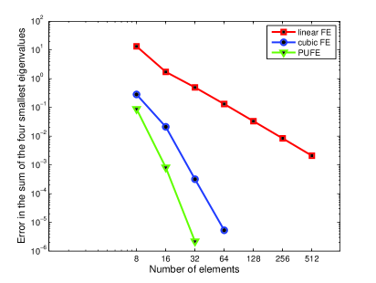
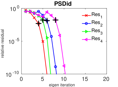
Figure 5.1: Left: error of the sum of four smallest eigenvalues of $(H,S)$ with respect to the number of FEs of three different FE discretizatoins in Example 5.1. Right: convergence of the PSD-id method for computing four smallest eigenvalues.

Example 5.2.

The Hermitian-definite generalized eigenvalue problem (1.1) is a computational kernel in quantum mechanical methods employing a nonorthogonal basis for ab initio three-dimensional electronic structure calculations, see [3] and references therein. In this example, we select a sequence of eigenproblems produced by the PUFE method for a self-consistent pseudopotential density functional calculation for metallic, triclinic CeAl [26, 23, 22]. The Brillouin zone is sampled at two ${\bf k}$-points: ${\bf k}=(0.00,\,0.00,\,0.00)$ and ${\bf k}=(0.12,\,-0.24,\,0.37)$. The PUFE approximation for the wavefunction is of the form given in the equation (5.6) and we apply a standard Galerkin procedure to set up the discrete system matrices. The unit cell is a triclinic box, with atoms displaced from ideal positions. The primitive lattice vectors and the position of the atomic centers are

$${\bf a}_{1}=a(1.00\quad 0.02\quad-0.04),\quad{\bf a}_{2}=a(0.01\quad 0.98\quad 0.03),\quad{\bf a}_{3}=a(0.03\quad-0.06\quad 1.09)$$

and

$${\bf\tau}_{\rm{Ce}}=a(0.01\quad 0.02\quad 0.03),\quad{\bf\tau}_{\rm{Al}}=a(0.51\quad 0.47\quad 0.55),$$

with lattice parameter $a=5.75$ bohr. Since Ce has a full complement of $s$, $p$, $d$, and $f$ states in valence, it requires 17 enrichment functions to span the occupied space. The near-dependencies between the finite element basis functions and the enriched basis functions lead to an ill-conditioned generalized eigenvalue problem (1.1).

In this numerical example, the matrix size of $H$ and $S$ is $n=7\times 8^{3}+1752=5336$. Both $H$ and $S$ are ill conditioned and their condition numbers are $(\kappa_{2}(H),\kappa_{2}(S))=(1.1641\times 10^{10},2.5731\times 10^{11})$. Furthermore, $H$ and $S$ share a common near-nullspace $\operatorname{span}(V)$ of dimension 1000 such that $\|HV\|=\|SV\|=O(10^{-4})$, where $V$ is orthonormal. This is an extremely ill-conditioned eigenvalue problem. Figure 5.2 shows the convergence history of the PSD-id method for computing four smallest eigenvalues. As in Figure 5.1, the localization of the $j$ approximate eigenpair $(\lambda_{i;j},u_{i;j})$ is marked by “+” sign. Once $\lambda_{i;j}$ is localized, the locally accelerated preconditioner ${\widetilde{K}}_{i;j}=(H-\lambda_{i;j}S)^{-1}$ is used. Again, as Theorem 4.1 predicts, the locally accelerated preconditioner ${\widetilde{K}}_{i;j}$ leads to superlinear convergence of the PSD-id algorithm.

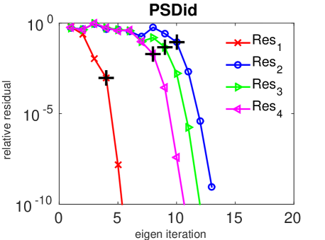
Figure 5.2: Convergence of the PSD-id method for computing four smallest eigenvalues of the CeAl matrix pair described in Example 5.2.

6 Conclusion

In this paper, we proved the convergence of the PSD-id method, and derived a nonasymptotic estimate of the rate of convergence of the method. We show that with the proper choice of the shift, the indefinite shift-and-invert preconditioner is a locally accelerated preconditioner and leads to superlinear convergence. Two numerical examples are presented to verify the theoretical results on the convergence behavior of the PSD-id method for solving ill-conditioned Hermitian-definite generalized eigenvalue problems.

References

• [1] J. H. Bramble, J. E. Pasciak, and A. V. Knyazev. A subspace preconditioning algorithm for eigenvector/eigenvalue computation. Adv. Comput. Math., 6(1):159–189, 1996.
• [2] B. R. Brooks, D. Janežič, and M. Karplus. Harmonic analysis of large systems. I. methodology. J. Comput. Chem., 16(12):1522–1542, 1995.
• [3] Y. Cai, Z. Bai, J. E. Pask, and N. Sukumar. Hybrid preconditioning for iterative diagonalization of ill-conditioned generalized eigenvalue problems in electronic structure calculations. J. Comput. Phys., 255:16 –30, 2013.
• [4] D. K. Fadeev and V. N. Fadeeva. Computational methods of linear algebra. W. H. Freeman, San Francisco and London, 1963.
• [5] G. Fix and R. Heiberger. An algorithm for the ill-conditioned generalized eigenvalue problem. SIAM J. Numer. Anal., 9(1):78–88, 1972.
• [6] D. J. Griffiths. Introduction to quantum mechanics (2nd Edition). Pearson Prentice Hall, 2004.
• [7] M. R. Hestenes and W. Karush. A method of gradients for the calculation of the characteristic roots and vectors of a real symmetric matrix. J. Res. Nat. Bur. Stand., 47(1):45–61, 1951.
• [8] T. Kato. Upper and lower bounds of eigenvalues. Phys. Rev., 77(3):413, 1950.
• [9] A. V. Knyazev and K. Neymeyr. Efficient solution of symmetric eigenvalue problems using multigrid preconditioners in the locally optimal block conjugate gradient method. Electron. Trans. Numer. Anal., 15:38–55, 2003.
• [10] M. Levitt. Private communication, January 2015.
• [11] M. Levitt, C. Sander, and P. S. Stern. Protein normal-mode dynamics: trypsin inhibitor, crambin, ribonuclease and lysozyme. J. Mol. Biol., 181(3):423–447, 1985.
• [12] R. L. Liboff. Introductory quantum mechanics (4th Edition). Addison-Wesley, 2003.
• [13] D. E. Longsine and S. F. McCormick. Simultaneous rayleigh-quotient minimization methods for Ax= $\lambda$Bx. Linear Algebra Appl., 34:195–234, 1980.
• [14] J. M. Melenk and I. Babuška. The partition of unity finite element method: basic theory and applications. Comput. Methods Appl. Mech. Engrg., 139(1):289–314, 1996.
• [15] K. Neymeyr and M. Zhou. The block preconditioned steepest descent iteration for elliptic operator eigenvalue problems. Electron. Trans. Numer. Anal., 41:93–108, 2014.
• [16] K. Neymeyr and M. Zhou. Iterative minimization of the rayleigh quotient by block steepest descent iterations. Numer. Linear Algebra Appl., 21(5):604–617, 2014.
• [17] T. Nishikawa and N. Gō. Normal modes of vibration in bovine pancreatic trypsin inhibitor and its mechanical property. Proteins: Struct., Funct., Bioinf., 2(4):308–329, 1987.
• [18] F. W. J. Olver. NIST handbook of mathematical functions. Cambridge University Press, 2010.
• [19] E. Ovtchinnikov. Cluster robustness of preconditioned gradient subspace iteration eigensolvers. Linear Algebra Appl., 415(1):140–166, 2006.
• [20] E. E. Ovtchinnikov. Sharp convergence estimates for the preconditioned steepest descent method for hermitian eigenvalue problems. SIAM J. Numer. Anal., 43(6):2668–2689, 2006.
• [21] C. C. Paige and M. A. Saunders. Solution of sparse indefinite systems of linear equations. SIAM J. Numer. Anal., 12(4):617–629, 1975.
• [22] J. E. Pask, N. Sukumar, M. Guney, and W. Hu. Partition-of-unity finite-element method for large scale quantum molecular dynamics on massively parallel computational platforms. Technical report, Technical Report LLNL-TR-470692, Department of Energy LDRD 08-ERD-052, 2011.
• [23] J. E. Pask, N. Sukumar, and S. E. Mousavi. Linear scaling solution of the all-electron Coulomb problem in solids. Int. J. Multiscale Comput. Eng., 10(1), 2012.
• [24] W. V. Petryshyn. On the eigenvalue problem Tu - $\lambda$ Su= 0 with unbounded and nonsymmetric operators T and S. Philos. Trans. R. Soc. Math. Phys. Sci., 262(1130):413–458, 1968.
• [25] B. A. Samokish. The steepest descent method for an eigenvalue problem with semi-bounded operators. Izv. Vyssh. Uchebn. Zaved. Mat., 5:105–114, 1958.
• [26] N. Sukumar and J. E. Pask. Classical and enriched finite element formulations for bloch-periodic boundary conditions. Int. J. Numer. Meth. Eng., 77(8):1121, 2009.
• [27] J. H. Wilkinson. The algebraic eigenvalue problem. 1965.