Optimal error analysis of a FEM for fractional diffusion problems by energy arguments

Abstract

In this article, the piecewise-linear finite element method (FEM) is applied to approximate the solution of time-fractional diffusion equations on bounded convex domains. Standard energy arguments do not provide satisfactory results for such a problem due to the low regularity of its exact solution. Using a delicate energy analysis, a priori optimal error bounds in $L^{2}(\Omega)$-, $H^{1}(\Omega)$-norms, and a quasi-optimal bound in $L^{\infty}(\Omega)$-norm are derived for the semidiscrete FEM for cases with smooth and nonsmooth initial data. The main tool of our analysis is based on a repeated use of an integral operator and use of a $t^{m}$ type of weights to take care of the singular behavior of the continuous solution at $t=0.$ The generalized Leibniz formula for fractional derivatives is found to play a key role in our analysis. Numerical experiments are presented to illustrate some of the theoretical results.

1 Introduction

In this paper, we investigate the error analysis via energy arguments of a semidiscrete Galerkin finite element method (FEM) for time-fractional diffusion problems of the form: find $u=u(x,t)$ such that

$$u^{\prime}(x,t)+\partial_{t}^{1-\alpha}{\cal{L}}u(x,t)=f(x,t)\quad\mbox{ in }\Omega\times(0,T],$$ (1)

with $u(x,0)=u_{0}(x)$ in $\Omega$, subject to homogeneous Dirichlet boundary conditions, that is, $u(x,t)=0$ on $\partial\Omega\times(0,T]$. Here ${\cal{L}}u=-{\rm div}({\bf a}(x)\nabla u)$, $\Omega$ is a bounded, convex polygonal domain in $\mathbb{R}^{2}$ with boundary $\partial\Omega$, $f$, ${\bf a}$ and $u_{0}$ are given functions defined on their respective domains. In (1), $u^{\prime}$ is the time partial derivative of $u$ and $\partial_{t}^{1-\alpha}:={{}^{R}}{\rm D}^{1-\alpha}$ is the Riemann–Liouville time-fractional derivative defined by: for $0<\alpha<1$,

$$\partial_{t}^{1-\alpha}\varphi(t):=\frac{\partial}{\partial t}\mathcal{I}^{\alpha}\varphi(t):=\frac{\partial}{\partial t}\int_{0}^{t}\omega_{\alpha}(t-s)\varphi(s)\,ds\quad\text{with}\quad\omega_{\alpha}(t):=\frac{t^{\alpha-1}}{\Gamma(\alpha)},$$ (2)

($\mathcal{I}^{\alpha}$ is the Riemann–Liouville time-fractional integral). We assume that the source term $f$ and the diffusivity coefficient function ${\bf a}$ are sufficiently regular and

$$0<a_{\min}\leq{\bf a}(x)\leq a_{\max}<\infty\quad{\rm on}~{}~{}\overline{\Omega}.$$ (3)

Several numerical techniques for the problem (1) (with constant diffusivity coefficient) in one and several space variables have been proposed with various types of spatial discretizations including finite difference, finite volume or spectral element methods, see CockburnMustapha2015 ; KMP2017 ; JLPZ2015 . For the time discretization, different time-stepping schemes (implicit and explicit) have been investigated including finite difference, convolution quadrature, and discontinuous Galerkin methods, see ChenLiuAnhTurner2012 ; CuestaLubichPalencia2006 ; Cui2012 ; Mustapha2011 ; RZ2013 ; ZS2011 . The error analyses in most studies in the existing literature typically assume that the solution $u$ of (1) is sufficiently regular including at $t=0$, which is not practically the case, see Mclean2010 . Indeed, assuming high regularity on $u$ imposes additional compatibility conditions on the given data, which are not reasonable in many cases.

Though the numerical approximation of the solution $u$ of (1) was considered by many authors over the last decade, the optimality of the estimates with respect to the solution smoothness expressed through the problem data, $f$ and $u_{0}$, was considered in a few papers for the case of constant diffusivity and quasi-uniform meshes. Obtaining sharp error bounds under reasonable regularity assumptions on $u$ has proved challenging. The first optimal $L^{2}(\Omega)$-error estimate for the Galerkin finite element solution of (1) with respect to the regularity of initial data was established MT2010a . More precisely, for $t\in(0,T]$, convergence rates of order $h^{2}t^{\alpha(\delta-2)/2}$ ($h$ denoting the maximum diameter of the spatial mesh elements) were proved assuming that the initial data $u_{0}\in\dot{H}^{\delta}(\Omega)$ for $\delta=0,\,2$ (see, Section 2 for the definition of these spaces). The proof was based on some refined estimates of the Laplace transform in time for the error. In MT2010b , by using a similar approach, the same authors derived $O(h^{2}\ell_{h}^{2}t^{-\alpha(2-\delta)/2})$ convergence rates in the stronger $L^{\infty}(\Omega)$-norm, where $\ell_{h}=\max\{1,|\log h|\}.$ For $\delta=0$, $u_{0}$ was assumed to be in $L^{\infty}(\Omega)$, while for $\delta=2$, $u_{0}$ was assumed to be in $C^{2}(\Omega)$ and vanishes on $\partial\Omega$. Recently, in McLeanMustapha2015 , the error analysis of a first order semidiscrete time-stepping scheme for problem (1) with $f\equiv 0$ allowing nonsmooth $u_{0},$ using discrete Laplace transform technique. Since standard energy arguments are used heavily in the error analysis of Galerkin FEMs for classical diffusion equations, it is more pertinent to extend the analysis to these time-fractional order diffusion problems with a variable diffusivity. Since $t^{m}$ and $\partial_{t}^{1-\alpha}{\cal{L}}$ do not commute, extending these arguments to problem (1) is not a straightforward task, especially in the case of nonsmooth $u_{0}$.

The main motivation of this work is to propose delicate energy arguments approach to derive optimal error estimates of the semidiscrete Galerkin FEM for the problem (1) for both smooth and nonsmooth initial data $u_{0}$. Earlier, for smooth $u_{0}$, a quasi-optimal error estimate of order $O(h^{2}\ell_{h})$ in $L^{\infty}(L^{2})$-norm was derived in MustaphaMcLean2011 using direct energy arguments. The proposed technique in this work has several advantages over the approaches used in MT2010a ; MT2010b to show optimal error bounds for smooth and nonsmooth $u_{0}$. Some of these are: (1) allowing variable coefficients, (2) the source term $f$ can depend on the unknown solution $u$, that is, the fractional diffusion problem (1) is semilinear (see Remark 1), (3) the quasi-uniform mesh assumption is not required to show the convergence results in $H^{m}$-norm for $m=0,1$, and (4) the proposed energy argument approach can be applied to other fractional diffusion problems. For instance, the achieved error bounds in Theorems 4.1, 5.2 and 5.3 can be extended to the time-fractional diffusion equation,

$${{}^{C}}\partial_{t}^{\alpha}u(x,t)+{\cal{L}}u(x,t)=f(x,t)\quad{\rm for}~{}~{}0<\alpha<1,$$ (4)

where ${{}^{C}}\partial_{t}^{\alpha}v(t):=\mathcal{I}^{1-\alpha}v^{\prime}(t)$ is the Caputo derivative. The error estimate in Theorem 4.1 provides an improvement of the result obtained in (JLZ2013, , Theorem 3.7). For constant diffusivity, using a semigroup approach and assuming that the mesh is quasi-uniform, the derived error bound therein involves a logarithmic factor.

Outline of the paper. In Section 2, we recall some smoothness properties of the solution $u$, we also state and derive some technical results. In Section 3, we introduce our semidiscrete finite element scheme and recall some error results. We claim that a direct application of energy arguments to problem (1) does not lead to optimal convergence rates even when the initial data $u_{0}\in\dot{H}^{2}(\Omega)$. In Section 4, for $t\in(0,T]$ and for $u_{0}\in\dot{H}^{\delta}(\Omega)$, an optimal error estimate in $L^{2}(\Omega)$-norm of order $h^{2}t^{-\alpha(2-\delta)/2}$ is established when $0\leq\delta\leq 2$, see Theorem 4.1. In Section 5, a superconvergence gradient error bound is obtained, see Theorem 5.1. As a consequence, an optimal $O(h\,t^{-\alpha(2-\delta)/2})$ estimate in the $H^{1}(\Omega)$-norm is derived for $0\leq\delta\leq 1,$ see Theorem 5.2. However, for $1<\delta\leq 2,$ we showed an $O(h\,t^{-\alpha(1-\delta)/2}\max\{1,(h/t)^{-\alpha(1-\delta)/2}\})$ error estimate, reduces to $h\,t^{-\alpha(2-\delta)/2}$ for $t=O(h)$. Furthermore, assuming that $u_{0}\in\dot{H}^{\delta}(\Omega)\cap L^{\infty}(\Omega)$ and the mesh is quasi-uniform, a quasi-optimal error estimate of order $h^{2}\ell_{h}^{5/2}t^{-\alpha(3-\delta)/2}$ in the stronger $L^{\infty}(\Omega)$-norm is proved in Theorem 5.3. Particularly relevant to this a priori error analysis is the appropriate use of several properties of the time-fractional integral and derivative operators. Numerical tests are presented in Section 6 to confirm some of our theoretical findings. Throughout the paper, $C$ is a generic positive constant that may depend on $\alpha$ and $T$, but is independent of $h$.

2 Regularity and technical results

Smoothness properties of the solution $u$ of the fractional diffusion problem (1) play a key role in the error analysis of the Galerkin FEM, particularly, since $u$ has singularity near $t=0$, even for smooth given data. Below, we state the required regularity results for problem (1) in terms of the initial data $u_{0}$ and the source term $f$. For $0\leq r,\,\mu\leq 2$,

$$t^{q}\|u^{(q)}(t)\|_{r+\mu}\leq C(1+T^{\alpha\mu/2})\,t^{-\alpha\mu/2}d_{r}(u_{0},f),\quad{\rm for}~{}~{}q\in\{0,1\},$$ (5)

with $r+\mu\leq 2$, where $d_{r}(u_{0},f)=\|u_{0}\|_{r}+\sum_{m=0}^{q+1}\int_{0}^{T}s^{m}\|f^{(m)}(s)\|_{r}\,ds.$ Here, $\|\cdot\|_{r}$ denotes the norm on the Hilbert space $\dot{H}^{r}(\Omega)$ defined by $\|v\|_{r}^{2}=\sum_{j=1}^{\infty}\lambda_{j}^{r}(v,\phi_{j})^{2},$ where $\{\lambda_{j}\}_{j=1}^{\infty}$ are the eigenvalues of the elliptic operator ${\cal{L}}$ (subject to homogeneous Dirichlet boundary conditions) and $\{\phi_{j}\}_{j=1}^{\infty}$ are the associated orthonormal eigenfunctions. Noting that, $\dot{H}^{r}(\Omega)=H^{r}(\Omega)$ for $0\leq r<1/2,$ $\dot{H}^{r}(\Omega)=\overline{C^{\infty}_{0}(\Omega)}$ in $H^{r}(\mathbb{R}^{2})$ for $r=1/2,$ and for convex polygonal domains, $\dot{H}^{r}(\Omega)=\{w\in H^{r}(\Omega):w=0~{}{\rm on}~{}\partial\Omega\}$ for $1/2<r\leq 2,$ where $H^{r}(\Omega)$ is the standard Sobolev space with $H^{0}(\Omega)=L^{2}(\Omega)$.

For constant diffusivity, over the convex domain $\Omega$, the regularity property (5) follows by combining the results of Theorems 4.1, 4.2 and 5.6 in Mclean2010 . In the proof, it was used that the operator ${\cal L}$ (subject to homogeneous Dirichlet) is positive definite and possess a complete eigensystem. These properties remain valid if the diffusivity coefficient function ${\bf a}$ is sufficiently regular and satisfies the positivity assumption (3).

Next, we state the positivity properties of the fractional operators $\mathcal{I}^{\alpha}$ and $\partial_{t}^{1-\alpha}$, and derive some technical results that will be used in the subsequent sections. By (MustaphaSchoetzau2014, , Lemma 3.1 (ii)), and since the bilinear form $A(\cdot,\cdot)$ associated with the operator ${\cal{L}}$ (that is, $A(v,w)=({\bf a}\nabla v,\nabla w)$) is symmetric positive definite on the Sobolev space $H_{0}^{1}(\Omega)$, it follows that for piecewise time continuous functions $\varphi:[0,T]\to H_{0}^{1}(\Omega),$

$$\int_{0}^{T}A(\mathcal{I}^{\alpha}\varphi,\varphi)\,dt\geq\cos(\alpha\pi/2)\int_{0}^{T}\|\sqrt{\bf a}\,\nabla\mathcal{I}^{\alpha/2}\varphi\|^{2}\,dt\geq 0~{}~{}{\rm for}~{}~{}0<\alpha<1,$$ (6)

where $\|\varphi\|:=\sqrt{(\varphi,\varphi)}$ denotes the $L^{2}(\Omega)$-norm. Furthermore, by (McLean2012, , Lemma A.1), the following holds: for $W^{1,1}(0,T;H_{0}^{1}(\Omega))$,

$$\int_{0}^{T}A(\partial_{t}^{1-\alpha}\varphi(t),\varphi(t))\,dt\geq\frac{1}{2}\sin(\alpha\pi/2)T^{\alpha-1}\int_{0}^{T}\|\sqrt{{\bf a}}\nabla\varphi(t)\|^{2}\,dt\,.$$ (7)

The next lemma will be used frequently in our convergence analysis. In the proof, we use the following integral inequality: if for any $\tau\in(0,t)$, $|\phi(\tau)|^{2}\leq|\phi(0)|^{2}+2\,\int_{0}^{\tau}|\phi(s)|\,|\psi(s)|\,ds,$ then $|\phi(t)|\leq|\phi(0)|+\int_{0}^{t}\,|\psi(s)|\,ds$, see (CockburnMustapha2015, , Lemma 4).

Lemma 1

Let $\kappa\in\{0,1\}$ and let ${\mathcal{B}}^{\alpha}=\partial_{t}^{1-\alpha}$ or ${\mathcal{B}}^{\alpha}=\mathcal{I}^{\alpha}.$ Assume that

$$\kappa(v(t),\chi)+(1-\kappa)(v^{\prime}(t),\chi)+A({\mathcal{B}}^{\alpha}v(t),\chi)=(w(t),\chi),\quad\forall~{}\chi\in V_{h},$$ (8)

for $t\in(0,T]$. Then

$$\kappa\int_{0}^{t}\|v\|^{2}\,ds+(1-\kappa)\|v(t)\|^{2}\leq(1-\kappa)\Big{(}\|v(0)\|+\int_{0}^{t}\|w\|\,ds\Big{)}^{2}+\kappa\int_{0}^{t}\|w\|^{2}\,ds.$$

Proof

Choose $\chi=v$ in (8), and then, integrate over the interval $(0,t)$ to obtain

$$2\kappa\int_{0}^{t}\|v\|^{2}\,ds+(1-\kappa)[\|v(t)\|^{2}-\|v(0)\|^{2}]+2\int_{0}^{t}A({\mathcal{B}}^{\alpha}v,v)ds=2\int_{0}^{t}(w,v)\,ds.$$

By the positivity properties in (6) and in (7), $\int_{0}^{t}A({\mathcal{B}}^{\alpha}v,v)ds\geq 0$, and thus,

$$2\kappa\int_{0}^{t}\|v\|^{2}\,ds+(1-\kappa)\|v(t)\|^{2}\leq(1-\kappa)\|v(0)\|^{2}+2\int_{0}^{t}\|w\|\,\|v\|\,ds.$$

Therefore, for $\kappa=0$, an application of the integral inequality (stated above) yields the desired inequality. However, for $\kappa=1$, we use the inequality $2\|w\|\,\|v\|\leq\|w\|^{2}+\|v\|^{2}$ and the desired result follows.$\quad\Box$

3 Semi-discrete FEM

This section focuses on a semidiscrete Galerkin FEM for problem (1). To define the scheme, let $\mathcal{T}_{h}$ be a family of regular triangulations (made of simplexes $K$) of the domain $\overline{\Omega}$ and let $h=\max_{K\in\mathcal{T}_{h}}(\mbox{diam}K),$ where $h_{K}$ denotes the diameter of the element $K.$ Let $V_{h}\subset H^{1}_{0}(\Omega)$ denote the usual space of continuous, piecewise-linear functions on $\mathcal{T}_{h}$ that vanish on $\partial\Omega$.

The weak formulation for problem (1) is to find $u:(0,T]\longrightarrow H^{1}_{0}(\Omega)$ such that

$$(u^{\prime},v)+A(\partial_{t}^{1-\alpha}u,v)=(f,v)\quad\forall v\in H^{1}_{0}(\Omega)$$ (9)

with given $u(0)=u_{0}.$ Thus, the standard semidiscrete finite element formulation for (1) is to seek $u_{h}:(0,T]\longrightarrow V_{h}$ such that

$$(u_{h}^{\prime},v_{h})+A(\partial_{t}^{1-\alpha}u_{h},v_{h})=(f,v_{h})\quad\forall v_{h}\in V_{h}$$ (10)

with given $u_{h}(0)\in V_{h}$ to be defined later.

To derive a priori error estimates for the numerical scheme (10), we split the error $e:=(u-R_{h}u)-(u_{h}-R_{h}u)=:\rho-\theta,$ where the Ritz projection $R_{h}:H_{0}^{1}(\Omega)\rightarrow V_{h}$ is defined by the following relation: $A(R_{h}v-v,\chi)=0$ for all $\chi\in V_{h}.$ For $t\in(0,T]$, the projection errors $\rho(t)$ and $\rho^{\prime}(t)$ satisfy the following estimates: for $j=0,1,$

$$\|\rho(t)\|_{j}\leq Ch^{m-j}\|u(t)\|_{m}~{}~{}{\rm and}~{}~{}\|\rho^{\prime}(t)\|_{j}\leq Ch^{m-j}\|u^{\prime}(t)\|_{m},~{}~{}{\rm for}~{}~{}m=1,2.$$ (11)

Hence, by using the regularity property in (5), we observe

$$\|\rho(t)\|+t\|\rho^{\prime}(t)\|\leq Ch^{m}t^{-\max\{0,\alpha(m-\delta)/2\}}d_{\delta}(u_{0},f),\quad{\rm for}~{}~{}0\leq\delta\leq 2.$$ (12)

Next, we show that a direct application of energy arguments to problem (1) does not yield satisfactory results due to the low regularity of the continuous solution. From (9) and (10), the error decomposition $e=\rho-\theta$, and the property of the elliptic projection, we obtain the equation in $\theta$ as

$$(\theta^{\prime},\chi)+A(\partial_{t}^{1-\alpha}\theta,\chi)=(\rho^{\prime},\chi)\quad\forall~{}\chi\in V_{h}.$$ (13)

Then, the following result holds (MustaphaMcLean2011, , Theorem 4): for $t\in(0,T],$ we have

$$\|u(t)-u_{h}(t)\|\leq\|\theta(0^{+})\|+\int_{0}^{t}\|\rho^{\prime}(s)\|\,ds+\|\rho(t)\|.$$ (14)

Practically, the solution $u$ has singularity near $t=0$. For instance, if $f\equiv 0$ and $u_{0}\in\dot{H}^{2}(\Omega)$, then $\|u^{\prime}(t)\|_{m}\leq Ct^{\alpha(2-m)/2-1}\|u_{0}\|_{2}$ for $m=1,2$, see Mclean2010 . Hence, by (11),

$$\int_{0}^{t}\|\rho^{\prime}(s) \|\,ds\leq Ch\int_{0}^{\epsilon}\|u^{\prime}(s)\|_{1}\,ds+Ch^{2}\int_{\epsilon}^{t}\|u^{\prime}(s)\|_{2}\,ds$$

$$\leq C\Big{(}h\int_{0}^{\epsilon}s^{\alpha/2-1}\,ds+h^{2}\int_{\epsilon}^{t}s^{-1}\,ds\Big{)}\|u_{0}\|_{2}\leq Ch^{2}\ell_{h}\|u_{0}\|_{2},~{}{\rm for}~{}\epsilon=h^{2/\alpha}.$$

This leads to a quasi-optimal $O(h^{2}\ell_{h})$ convergence. To achieve an optimal $O(h^{2})$ convergence, a stronger regularity assumption on $u$ is required and that, in turn imposes severe restrictions on the initial data $u_{0}$. Thus, the error bound in (14) is not sharp even for the case of smooth $u_{0}$, that is, $H^{2}$-regularity on $u_{0}$ is not sufficient to get an optimal $O(h^{2})$ convergence rate. Furthermore, it is clear that this upper bound is not suitable for the case of nonsmooth $u_{0}$. Therefore, we propose in the next section an approach via delicate energy arguments that provides optimal error bounds for both cases: smooth and nonsmooth $u_{0}$.

Remark 1

Our forthcoming convergence analysis can be easily extended if the source term $f=f(x,t,u(x,t))$ in the problem (1), assuming that $f$ is sufficiently regular in the three variables and satisfies that $|f(x,t,z_{1})-f(x,t,z_{2})|\leq C|z_{1}-z_{2}|$ for $z_{1},z_{2}\in\mathbb{R}$ (that is, $f$ is Lipschitz continuous in the third variable). Studying the regularity properties of the continuous solution $u$ remains an open problem in this case.

The spatial finite element scheme for (1) is: find $u_{h}:(0,T]\longrightarrow V_{h}$ such that

$$(u_{h}^{\prime},v_{h})+A(\partial_{t}^{1-\alpha}u_{h},v_{h})=(f(u_{h}),v_{h})\quad\forall~{}v_{h}\in V_{h}$$

with given $u_{h}(0)\in V_{h}$. Hence, instead of (13), we have

$$(\theta^{\prime},\chi)+A(\partial_{t}^{1-\alpha}\theta,\chi)=(\rho^{\prime}+[f(u_{h})-f(u)],\chi)\quad\forall~{}\chi\in V_{h}.$$

We follow the proofs in Sections 4 and 5 step-by-step where the term $\rho(t)$ will be replaced with $\tilde{\rho}(t):=\rho(t)+\int_{0}^{t}[f(u_{h})-f(u)]\,ds$ and the Lipschitz continuity property of $f$ will be used appropriately.$\quad\Box$

4 $L^{2}(\Omega)$-error estimates

For convenience, we introduce the notations:

$$\Theta_{i}(t):=t^{i}\theta(t)\quad{\rm and}\quad\dot{\Theta}_{i}(t):=t^{i}\theta^{\prime}(t)~{}~{}{\rm for}~{}~{}i=1,\,2.$$

In the next lemma, based on the generalized Leibniz formula for fractional derivatives, we state and show some identities for our subsequent use.

Lemma 2

For $0<\alpha<1$, the followings hold:
(a) $t\partial_{t}^{1-\alpha}\theta=\partial_{t}^{1-\alpha}\Theta_{1}-(1-\alpha)\mathcal{I}^{\alpha}\theta$,
(b) $t\mathcal{I}^{\alpha}\theta=\mathcal{I}^{\alpha}\Theta_{1}+\alpha\mathcal{I}^{1+\alpha}\theta$.

Proof

The first identity follows from the fractional Leibniz formula. To show the second identity, noting first that $\partial_{t}^{1-\alpha}\Theta_{1}=\mathcal{I}^{\alpha}\Theta^{\prime}_{1}=\mathcal{I}^{\alpha}\theta+\mathcal{I}^{\alpha}\dot{\Theta}_{1}.$ Hence, by (a),

$$t\partial_{t}^{1-\alpha}\theta(t)=\mathcal{I}^{\alpha}\dot{\Theta}_{1}(t)+\alpha\mathcal{I}^{\alpha}\theta(t).$$ (15)

Now, we replace $\theta$ by $\mathcal{I}\theta$ in (15) to obtain the second identity in the lemma.$\quad\Box$

Next, we derive an upper bound of $\Theta_{1}$. To do so, we let $u_{h}(0)=P_{h}u_{0},$ where $P_{h}:L^{2}(\Omega)\rightarrow V_{h}$ denotes the $L^{2}$-projection defined by $(P_{h}v-v,\chi)=0$ for all $\chi\in V_{h}.$

Lemma 3

Let $u_{h}(0)=P_{h}u_{0}.$ Then, we have

$$\int_{0}^{t}\|\Theta_{1}\|^{2}\,ds\leq 3\int_{0}^{t}\Big{(}s^{2}\|\rho\|^{2}+2\big{(}\mathcal{I}\|\rho\|\big{)}^{2}\Big{)}\,ds,\quad{\rm for}~{}~{}t\in(0,T].$$

Proof

We integrate (13) over the time interval $(0,t)$ and obtain

$$(\theta,\chi)+A(\mathcal{I}^{\alpha}\theta-\mathcal{I}^{\alpha}\theta(0^{+}),\chi)=(\rho+e(0),\chi)\quad\forall~{}\chi\in V_{h}.$$ (16)

However, $A(\mathcal{I}^{\alpha}\theta(0^{+}),\chi)=-A(\mathcal{I}^{\alpha}e(0),\chi)$ for $\chi\in V_{h}$, and $\mathcal{I}^{\alpha}e(0)=0$ because $u$ and $u_{h}$ are both continuous on the time interval $[0,T]$. Furthermore, $(e(0),\chi)=0$ due to the equality $u_{h}(0)=P_{h}u_{0}.$ Therefore,

$$(\theta,\chi)+A(\mathcal{I}^{\alpha}\theta,\chi)=(\rho,\chi)\quad\forall~{}\chi\in V_{h}.$$ (17)

Multiply by $t$ and use $t\mathcal{I}^{\alpha}\theta=\mathcal{I}^{\alpha}\Theta_{1}+\alpha\mathcal{I}^{1+\alpha}\theta$ by Lemma 2 (b) to find that

$$(\Theta_{1},\chi)+A(\mathcal{I}^{\alpha}\Theta_{1},\chi)=t(\rho,\chi)-\alpha A(\mathcal{I}^{1+\alpha}\theta,\chi)\quad\forall~{}\chi\in V_{h}.$$

However, from (17), we get

$$A(\mathcal{I}^{\alpha+1}\theta,\chi)=(\mathcal{I}(\rho-\theta),\chi)\quad\forall~{}\chi\in V_{h},$$ (18)

and thus,

$$(\Theta_{1},\chi)+A(\mathcal{I}^{\alpha}\Theta_{1},\chi)=t(\rho,\chi)-\alpha(\mathcal{I}(\rho-\theta),\chi)\quad\forall~{}\chi\in V_{h}.$$ (19)

Consequently, an application of Lemma 1 (with $\kappa=1$) yields

$$\int_{0}^{t}\|\Theta_{1}\|^{2}\,ds\leq\int_{0}^{t}\|s\rho-\alpha\mathcal{I}(\rho-\theta)\|^{2}\,ds\leq 3\int_{0}^{t}(s^{2}\|\rho\|^{2}+\|\mathcal{I}\rho\|^{2}+\|\mathcal{I}\theta\|^{2})\,ds.$$ (20)

To complete our proof, we rewrite (18) as

$$(\mathcal{I}\theta,\chi)+A(\mathcal{I}^{\alpha}(\mathcal{I}\theta),\chi)=(\mathcal{I}\rho,\chi)\quad\forall~{}\chi\in V_{h},$$

Again, an application of Lemma 1 (with $\kappa=1$) shows

$$\int_{0}^{t}\|\mathcal{I}\theta\|^{2}\,ds \leq\int_{0}^{t}\|\mathcal{I}\rho\|^{2}\,ds.$$ (21)

Substitute (21) in (20) yields the desired bound.$\quad\Box$

An upper bound of the term $\theta$ will be derived in the next lemma. Again, for convenience, we introduce the following notation

$${\mathcal{B}}_{1}(t):=\int_{0}^{t}\Big{(}s^{4}\|\rho^{\prime}(s)\|^{2}+s^{2}\|\rho(s)\|^{2}+2\big{(}\mathcal{I}\|\rho(s)\|\big{)}^{2}\Big{)}\,ds\,.$$ (22)

For later use, by using the projection error estimates in (12) (with $m=2$) for upper bounds of $\rho$ and $\rho^{\prime}$, and then integrating, we find that for $t\in(0,T]$,

$${\mathcal{B}}_{1}(t)\leq C\,h^{4}t^{3-\alpha(2-\delta)}d_{\delta}^{2}(u_{0},f),\quad{\rm for}~{}~{}0\leq\delta\leq 2\,.$$ (23)

Lemma 4

Let $u_{h}(0)=P_{h}u_{0}$. Then, the following estimate holds

$$\|\theta(t)\|^{2}\leq C\,t^{-3}{\mathcal{B}}_{1}(t),\quad{\rm for}~{}~{}t\in(0,T]\,.$$

Proof

We multiply (13) by $t^{2}$ so that

$$(\dot{\Theta}_{2},\chi)+A(t^{2}\partial_{t}^{1-\alpha}\theta,\chi)=(t^{2}\rho^{\prime},\chi),$$ (24)

where $\dot{\Theta}_{2}=t^{2}\theta^{\prime}.$ From the fractional Leibniz formula, we have

$$t^{2}\partial_{t}^{1-\alpha}\theta =\partial_{t}^{1-\alpha}\Theta_{2}-2(1-\alpha)t\mathcal{I}^{\alpha}\theta+\alpha(1-\alpha)\mathcal{I}^{1+\alpha}\theta.$$

Hence, we rearrange (24) as

$$(\dot{\Theta}_{2},\chi)+A(\partial_{t}^{1-\alpha}\Theta_{2},\chi)=(t^{2}\rho^{\prime},\chi)+(1-\alpha)\Big{(}2tA(\mathcal{I}^{\alpha}\theta,\chi)-\alpha A(\mathcal{I}^{1+\alpha}\theta,\chi)\Big{)},$$ (25)

and then, by equations (17) and (18),

$$(\Theta_{2}^{\prime},\chi)+A(\partial_{t}^{1-\alpha}\Theta_{2},\chi)=(t^{2}\rho^{\prime}+2\alpha\Theta_{1}+(1-\alpha)(2t\rho-\alpha\mathcal{I}(\rho-\theta)),\chi).$$ (26)

Hence, by Lemma 1 (with $\kappa=0$), we obtain

$$\|\Theta_{2}(t)\| \leq\int_{0}^{t}\Big{(}s^{2}\|\rho^{\prime}(s)\|+2s\|\rho(s)\|+2\|\Theta_{1}(s)\|+\|\mathcal{I}(\rho-\theta)\|\Big{)}\,ds\,,$$

and thus, an application of the Cauchy-Schwarz inequality yields

$$\|\Theta_{2}(t)\|^{2} \leq Ct\int_{0}^{t}\Big{(}s^{4}\|\rho^{\prime}(s)\|^{2}+s^{2}\|\rho(s)\|^{2}+\|\Theta_{1}(s)\|^{2}+\|\mathcal{I}\rho\|^{2}+\|\mathcal{I}\theta\|^{2}\Big{)}\,ds\,.$$

Therefore, by using the identity $\theta(t)=t^{-2}\Theta_{2}(t)$, the inequality in (21) and Lemma 3 will complete the rest of the proof. $\quad\Box$

In the next theorem, we derive optimal convergence results of the finite element (10) in the $L^{2}(\Omega)$-norm for both smooth and nonsmooth initial data $u_{0}$. For $u_{0}\in\dot{H}^{\delta}(\Omega)$ with $0\leq\delta\leq 2,$ we show that the error is bounded by $Ch^{2}t^{-\alpha(2-\delta)/2}$ for each $t\in(0,T]$. Recall that, $\dot{H}^{\delta}(\Omega)=\{v\in H^{\delta}(\Omega):~{}v=0~{}{\rm on}~{}\partial\Omega\}$ for $1/2<\delta\leq 2$, while $\dot{H}^{\delta}(\Omega)=H^{\delta}(\Omega)$ for $0\leq\delta<1/2$.

Theorem 4.1

Let $u$ and $u_{h}$ be the solutions of $(\ref{a})$ and $(\ref{semi})$, respectively, with $u_{h}(0)=P_{h}u_{0}$. Then,

$$\|(u-u_{h})(t)\|\leq Ch^{2}t^{-\alpha(2-\delta)/2}d_{\delta}(u_{0},f)\quad{\rm for}~{}~{}t\in(0,T]~{}~{}{\rm with}~{}~{}0\leq\delta\leq 2\,.$$

Proof

The desired result follows from the decomposition $u-u_{h}=\rho-\theta$, the estimate of $\theta$ in Lemma 4, the bound in (23), and the estimate of $\rho$ in (12). $\quad\Box$

Remark 2

In the proof of the above theorem, we used (23) which follows from the projection estimate in (12) for $m=2.$ For $m=1$, we follow similar steps where $2-\delta$ will be replaced with $1-\delta$, to obtain ${\mathcal{B}}_{1}(t)\leq C\,h^{2}t^{3-\alpha(1-\delta)}d_{\delta}^{2}(u_{0},f)$ for $0\leq\delta\leq 1\,.$ Now, for $1<\delta\leq 2$, we notice first that for $0\leq q\leq t$ with $t_{h}=\max\{t,h\}$,

$$\|\rho(q)\|\leq\|\rho(t_{h})-\rho(q)\|+\|\rho(t_{h})\|\leq\mathcal{I}(\|\rho^{\prime}(t_{h})\|)+\|\rho(t_{h})\|\,.$$

Substituting this in the definition of ${\mathcal{B}}_{1}$ defined in (22), we observe

$${\mathcal{B}}_{1}(t)\leq Ct^{2}\int_{0}^{t}s^{2}\|\rho^{\prime}(s)\|^{2}\,ds+Ct^{3}\Big{(}\mathcal{I}(\|\rho^{\prime}(t_{h})\|)+\|\rho(t_{h})\|\Big{)}^{2}\,.$$

To estimate the first two terms, we use (11) (with $m=1$) and the following regularity property (which follows from (Mclean2010, , Theorems 4.2 and 5.6))

$$t\|u^{\prime}(t)\|_{1}\leq Ct^{\alpha(r-1)/2}\tilde{d}_{r}(u_{0},f),\quad t\in(0,T],\quad{\rm for}~{}~{}0\leq r\leq 2,$$ (27)

where $\tilde{d}_{r}(u_{0},f)=\|u_{0}\|_{r}+\sum_{j=0}^{2}\int_{0}^{T}s^{j+\alpha(1-r)/2}\|f^{(j)}(s)\|_{r}\,ds,$ we arrive to

$${\mathcal{B}}_{1}(t)\leq Ct^{3}h^{2}t_{h}^{\alpha(\delta-1)}\tilde{d}_{\delta}(u_{0},f)+Ct^{3}\|\rho(t_{h})\|^{2},\quad{\rm for}~{}~{}1<\delta\leq 2\,.$$

However, by (12) and the inequality $t_{h}^{-\alpha/2}\leq h^{-\alpha/2}$, we find that

$$\|\rho(t_{h})\|\leq Ch^{2}t_{h}^{\alpha(\delta-2)/2}d_{\delta}(u_{0},f)\leq Ch^{2-\alpha/2}t^{\alpha(\delta-1)/2}(t_{h}/t)^{\alpha(\delta-1)/2}d_{\delta}(u_{0},f).$$

Therefore,

$${\mathcal{B}}_{1}(t)\leq Ch^{2}t^{3+\alpha(\delta-1)}(t_{h}/t)^{\alpha(\delta-1)}\tilde{d}^{2}_{\delta}(u_{0},f),\quad{\rm for}~{}~{}1<\delta\leq 2\,.$$

Consequently, by using the above bound of ${\mathcal{B}}_{1}$ in Theorem 4.1, we get the error estimate below that will be used in the forthcoming section to show the convergence of the gradient finite element solution:

$$\|e(t)\|\leq Ch\,t^{-\alpha(1-\delta)/2}D_{\delta,\alpha}(u_{0},f,h/t),\quad{\rm for}~{}~{}~{}t\in(0,T],$$ (28)

where $D_{\delta,\alpha}(u_{0},f,h/t)=\tilde{d}_{\delta}(u_{0},f)$ for $0\leq\delta\leq 1$, while for $1<\delta\leq 2,$ $D_{\delta,\alpha}(u_{0},f,h/t)=\tilde{d}_{\delta}(u_{0},f)(t_{h}/t)^{\alpha(\delta-1)/2}$. $\quad\Box$

Remark 3

Under the quasi-uniformity condition on $V_{h}$, for $t\in(0,T]$, from the decomposition $u-u_{h}=\rho-\theta$, the inverse inequality, the estimate of $\theta$ in Lemma 4, and the estimate $\|\rho(t)\|_{1}\leq Ch\|u(t)\|_{2}\leq Ct^{-\alpha(2-\delta)/2}d_{\delta}(u_{0},f)$ (follows from the Ritz projection bound in (11) with $j=1$ and $m=2$ and the regularity property (5)), we obtain the following optimal error estimate:

$$\|\nabla(u-u_{h})(t)\|\leq Ch\,t^{-\alpha(2-\delta)/2}d_{\delta}(u_{0},f)\quad{\rm for}~{}~{}t\in(0,T]~{}~{}{\rm with}~{}~{}0\leq\delta\leq 2\,.$$

This error bound remains valid for $0\leq\delta\leq 1$ in the absence of the quasi-uniformity mesh assumption, see Theorem 5.2.$\quad\Box$

Remark 4

For smooth initial data $u_{0}\in{\dot{H}}^{2}(\Omega)$, one may choose $u_{h}(0)=R_{h}u_{0}$. An optimal convergence rate can be shown by following the proof of Theorem 4.1 line-by-line, where the term $\rho$ in Lemma 3 should be replaced with $\tilde{\rho}:=\rho+e(0)$. $\quad\Box$

5 $H^{1}(\Omega)$- and $L^{\infty}(\Omega)$-error estimates

In this section, we show optimal convergence error results in the $H^{1}(\Omega)$-norm, and quasi-optimal error bounds in the $L^{\infty}(\Omega)$-norm, for both smooth and nonsmooth initial data $u_{0}.$ We start our analysis by deriving an upper bound of $\nabla\Theta_{1}$.

Lemma 5

For $0\leq\delta\leq 2$ and for $t\in(0,T]$, we have

$$\int_{0}^{t}\|\nabla\Theta_{1}\|^{2}ds\leq Ch^{4}t^{3-\alpha(3-\delta)}d^{2}_{\delta}(u_{0},f)\,.$$

Proof

Multiplying (13) by $t$ and then using the first identity in Lemma 2,

$$(\dot{\Theta}_{1},\chi)+A(\partial_{t}^{1-\alpha}\Theta_{1},\chi)=(t\rho^{\prime},\chi)+(1-\alpha)A(\mathcal{I}^{\alpha}\theta,\chi).$$ (29)

Then, a use of (17) yields after simplifying

$$(\Theta_{1}^{\prime},\chi)+A(\partial_{t}^{1-\alpha}\Theta_{1},\chi)=((t\rho)^{\prime},\chi)-\alpha(e,\chi)\,.$$ (30)

Now, set $\chi=\Theta_{1}$ in (30), integrate the resulting equation over $(0,t)$, and use the positivity property of $\partial_{t}^{1-\alpha}$ in (7), to find that

$$\|\Theta_{1}(t)\|^{2}+\frac{1}{2}\sin(\alpha\pi/2)t^{\alpha-1}\int_{0}^{t}\|\sqrt{{\bf a}}\nabla\Theta_{1}\|^{2}\,ds\leq\int_{0}^{t}(\|(s\rho)^{\prime}\|+\|e\|)\|\Theta_{1}\|\,ds.$$ (31)

This implies

$$\|\Theta_{1}(t)\|^{2} \leq\int_{0}^{t}(\|(s\rho^{\prime})\|+\|e\|)\|\Theta_{1}\|\,ds.$$

By the integral inequality (stated before Lemma 1), we observe

$$\|\Theta_{1}(t)\| \leq\frac{1}{2}\int_{0}^{t}\big{(}\|(s\rho)^{\prime}\|+\|e\|\big{)}\,ds.$$

Substitute this bound in the RHS of (31) yields

$$\sin(\alpha\pi/2)t^{\alpha-1}\int_{0}^{t}\|\sqrt{{\bf a}}\nabla\Theta_{1}\|^{2}\,ds\leq\Big{(}\int_{0}^{t}\big{(}\|(s\rho)^{\prime}\|+\|e\|\big{)}ds\Big{)}^{2}.$$ (32)

Therefore, the desired estimate follows from this bound, the error projection in (12) (with $m=2$), the convergence results in Theorem 4.1, and (3).$\quad\Box$

In the next theorem, we derive an error bound for $\nabla\theta(t)$ in the $L^{2}(\Omega)$-norm.

Theorem 5.1

For $0\leq\delta\leq 2$, we have

$$\|\nabla\theta(t)\|^{2}\leq Ch^{4}t^{-\alpha(3-\delta)}d_{\delta}^{2}(u_{0},f),\quad{\rm for}~{}~{}t\in(0,T]\,.$$

Proof

We start by applying the operator $\mathcal{I}^{1-\alpha}$ to both sides of the elementary identity $\partial_{t}^{1-\alpha}\Theta_{2}(t)=\mathcal{I}^{\alpha}\Theta_{2}^{\prime}(t)+\omega_{\alpha}(t)\Theta_{2}(0^{+}),$ to notice that

$$\mathcal{I}^{1-\alpha}\partial_{t}^{1-\alpha}\Theta_{2}(t) =\mathcal{I}^{1-\alpha}\mathcal{I}^{\alpha}\Theta_{2}^{\prime}(t)+\mathcal{I}^{1-\alpha}\omega_{\alpha}(t)\Theta_{2}(0^{+})$$ (33)

$$=\Theta_{2}(t)-\Theta_{2}(0^{+})+\Theta_{2}(0^{+})=\Theta_{2}(t).$$

Now, applying again the operator $\mathcal{I}^{1-\alpha}$ to both sides (25), and using the above equality as well as the identity $t\mathcal{I}^{\alpha}\theta=\mathcal{I}^{\alpha}\Theta_{1}+\alpha\mathcal{I}^{1+\alpha}\theta$ (by Lemma 2 (b)) to get

$$(\mathcal{I}^{1-\alpha}\dot{\Theta}_{2},\chi)+A(\Theta_{2},\chi)=(\mathcal{I}^{1-\alpha}(t^{2}\rho^{\prime}),\chi)+(1-\alpha)\Big{(}2A(\mathcal{I}\Theta_{1},\chi)+\alpha A(\mathcal{I}^{2}\theta,\chi)\Big{)}.$$

Set $\chi=\dot{\Theta}_{2}$ follows by integrating the resulting equation from 0 to $t$ to obtain

$$\int_{0}^{t}[(\mathcal{I}^{1-\alpha} \dot{\Theta}_{2},\dot{\Theta}_{2})+A(\Theta_{2},\dot{\Theta}_{2})]\,ds$$

$$\leq\int_{0}^{t}(\mathcal{I}^{1-\alpha}(s^{2}\rho^{\prime}),\dot{\Theta}_{2})\,ds+(1-\alpha)\int_{0}^{t}A(2\mathcal{I}\Theta_{1}+\alpha\mathcal{I}^{2}\theta,\dot{\Theta}_{2})\,ds.$$

However, by the continuity property of the operator $\mathcal{I}^{1-\alpha}$ in (MustaphaSchoetzau2014, , Lemma 3.1),

$$\Big{|}\int_{0}^{t}(\mathcal{I}^{1-\alpha}(s^{2}\rho^{\prime}),\dot{\Theta}_{2})\,ds\Big{|}\leq C\int_{0}^{t}(\mathcal{I}^{1-\alpha}(s^{2}\rho^{\prime}),s^{2}\rho^{\prime})\,ds+\int_{0}^{t}(\mathcal{I}^{1-\alpha}\dot{\Theta}_{2},\dot{\Theta}_{2})\,ds,$$

and so,

$$\int_{0}^{t}A(\Theta_{2},\dot{\Theta}_{2})\,ds\leq C\int_{0}^{t}(\mathcal{I}^{1-\alpha}(s^{2}\rho^{\prime}),s^{2}\rho^{\prime})\,ds+(1-\alpha)\int_{0}^{t}A(2\mathcal{I}\Theta_{1}+\alpha\mathcal{I}^{2}\theta,\dot{\Theta}_{2})\,ds.$$

Using the identity $2\mathcal{I}\Theta_{1}(t)=\Theta_{2}(t)-\mathcal{I}\dot{\Theta}_{2}(t)$ and the inequality $\int_{0}^{t}A(\mathcal{I}\dot{\Theta}_{2},\dot{\Theta}_{2})\,ds\geq 0$, after some simplifications, we conclude that

$$\alpha\int_{0}^{t}A(\Theta_{2},\dot{\Theta}_{2})\,ds\leq C\int_{0}^{t}\|\mathcal{I}^{1-\alpha}s^{2}\rho^{\prime}\|\,\|s^{2}\rho^{\prime}\|\,ds+\alpha(1-\alpha)\int_{0}^{t}A(\mathcal{I}^{2}\theta,\dot{\Theta}_{2})\,ds.$$

Since

$$\int_{0}^{t}A(\Theta_{2},\dot{\Theta}_{2})\,ds=\frac{1}{2}\|\sqrt{{\bf a}}\nabla\Theta_{2}(t)\|^{2}-2\int_{0}^{t}s\|\sqrt{{\bf a}}\nabla\Theta_{1}(s)\|^{2}\,ds,$$

we easily find that

$$\alpha\|\sqrt{{\bf a}}\nabla\Theta_{2}(t)\|^{2}\leq 4\alpha\int_{0}^{t}s\|\sqrt{{\bf a}}\nabla\Theta_{1}(s)\|^{2}\,ds\\ +C\int_{0}^{t}\|\mathcal{I}^{1-\alpha}s^{2}\rho^{\prime}\|\,\|s^{2}\rho^{\prime}\|\,ds+2\alpha(1-\alpha)\int_{0}^{t}A(\mathcal{I}^{2}\theta,\dot{\Theta}_{2})\,ds.$$ (34)

By Lemma 5,

$$\int_{0}^{t}s\|\sqrt{{\bf a}}\nabla\Theta_{1}\|^{2}\,ds\leq Ct\int_{0}^{t}\|\nabla\Theta_{1}\|^{2}\,ds\leq Ch^{4}t^{4-\alpha(3-\delta)}d^{2}_{\delta}(u_{0},f)\,.$$ (35)

To estimate the second term on the RHS of (34), we use the bound of $\rho^{\prime}$ given in (12) (with $m=2$), the formula

$$\mathcal{I}^{\nu}(t^{\mu-1})=t^{\nu+\mu-1}\Gamma(\mu),\quad{\rm for}~{}~{}\nu,\,\mu>0,$$ (36)

and then integrate

$$\int_{0}^{t}(\mathcal{I}^{1-\alpha}(s^{2}\rho^{\prime}),s^{2}\rho^{\prime})\,ds\leq Ch^{4}\int_{0}^{t}s^{2-\alpha-\alpha(2-\delta)/2}s^{1-\alpha(2-\delta)/2}\,ds\,d^{2}_{\delta}(u_{0},f)\\ \leq Ch^{4}t^{4-\alpha-\alpha(2-\delta)}d^{2}_{\delta}(u_{0},f)\,.$$ (37)

For the last term on the RHS of (34), we apply $\mathcal{I}^{2-\alpha}$ to (17) to obtain $A(\mathcal{I}^{2}\theta,\chi)=(\mathcal{I}^{2-\alpha}e,\chi).$ Hence, integrating by parts, we find that

$$\int_{0}^{t}A(\mathcal{I}^{2}\theta,\dot{\Theta}_{2})\,ds =\int_{0}^{t}(s^{2}\mathcal{I}^{2-\alpha}e,\theta^{\prime})\,ds$$

$$=(\mathcal{I}^{2-\alpha}e(t),\Theta_{2}(t))-\int_{0}^{t}(2\mathcal{I}^{2-\alpha}e+s\mathcal{I}^{1-\alpha}e,\Theta_{1})\,ds\,.$$

Then, by using the estimate of $\theta$ in Lemma 4, (23), and the estimate of $e$ in Theorem 4.1, we conclude after integrating and using the formula in (36), that

$$\Big{|}\int_{0}^{t}A(\mathcal{I}^{2}\theta,\dot{\Theta}_{2})\,ds\Big{|} \leq t^{2}\|\mathcal{I}^{2-\alpha}e(t)\|\,\|\theta(t)\|+2t\int_{0}^{t}\|\mathcal{I}^{2-\alpha}e+s\mathcal{I}^{1-\alpha}e\|\,\|\theta\|\,ds$$

$$\leq Ch^{4}t^{4-\alpha-\alpha(2-\delta)}d_{\delta}^{2}(u_{0},f)\,.$$

A substitution of the estimates (35), (37) and the above one in (34), follows by using (3) and the identity $\theta(t)=t^{-2}\Theta_{2}$ yield the desired estimate. $\quad\Box$

Noting that, by using the estimates of $\rho$, $\rho^{\prime}$ and $e$ from Remark 2 in the inequality (32), we observe

$$\int_{0}^{t}\|\nabla\Theta_{1}\|^{2}ds\leq Ch^{2}t^{3-\alpha(2-\delta)}D^{2}_{\delta,\alpha}(u_{0},f,h/t)\,.$$

Hence, by following the steps in Theorem 5.1, and using the above bound instead of Lemma 5, and the bounds of $\rho^{\prime}$ and $e$ achieved in Remark 2, we deduce that

$$\|\nabla\theta(t)\|^{2}\leq C\,h^{2}\,t^{-\alpha(2-\delta)}D^{2}_{\delta,\alpha}(u_{0},f,h/t)\,.$$

Therefore, from the inequality $\|\nabla(u_{h}-u)(t)\|\leq\|\nabla\theta(t)\|+\|\nabla\rho(t)\|$, the above bound, the bound of $\eta$ in (11) (with $j=1$ and $m=2$) and the regularity property (5), we have the following result.

Theorem 5.2

Let $u$ and $u_{h}$ be the solutions of $(\ref{a})$ and $(\ref{semi})$, respectively, with $u_{h}(0)=P_{h}u_{0}$. For $u_{0}\in\dot{H}^{\delta}(\Omega)$, for $t\in(0,T]$, we have

$$\|\nabla(u-u_{h})(t)\|\leq C\,h\,t^{-\alpha(2-\delta)/2}\tilde{d}_{\delta}(u_{0},f)\times\begin{cases}1,~{}~{}~{}&~{}~{}0\leq\delta\leq 1,\\ \max\{1,(h/t)^{\alpha(\delta-1)/2}\},~{}~{}~{}&~{}~{}1<\delta\leq 2\,.\end{cases}$$

Remark 5

The estimate in Theorem 5.1 suggests that one can achieve a higher convergence rate for $\nabla(u_{h}-u)$ if an improved estimate of the error $\nabla(R_{h}u-u)$ can be derived. This could be achieved using a superconvergent recovery procedure of the gradient, which is possible on special meshes and for solutions in $H^{3}(\Omega)$ for each $t\in(0,T]$. Examples of special meshes exhibiting superconvergence property are provided in MN-87 . Therein, the authors introduced an operator $G_{h}$ which postprocesses $\nabla R_{h}u(t)$ with the following properties:

• If $u(t)\in H^{3}(\Omega)$, then $\|\nabla u(t)-G_{h}(R_{h}u)(t)\|\leq Ch^{2}\|u(t)\|_{H^{3}(\Omega)}.$

• For $\chi\in V_{h}$, we have $\|G_{h}(\chi)\|\leq C\|\nabla\chi\|.$

Now, if ${\cal T}_{h}$ is a triangulation of $\Omega$ such that these results are satisfied, then using

$$\|\nabla(u-u_{h})(t)\|\leq\|(\nabla u-G_{h}(R_{h}u))(t)\|+\|G_{h}(R_{h}u-u_{h})(t)\|+\|\nabla\theta(t)\|,$$

(i) and (ii), Theorem 5.1, and the inequality $\|u(t)\|_{H^{3}(\Omega)}\leq Ct^{-\alpha(3-\delta)/2}d_{\delta}(u_{0},f)$ for $1/2<\delta\leq 2$, it is clear that the bound below holds for $t\in(0,T]$,

$$\|\nabla(u-u_{h})(t)\|\leq Ch^{2}t^{-\alpha(3-\delta)/2}d_{\delta}(u_{0},f),\qquad 1/2<\delta\leq 2\,.\quad\Box$$

For $t\in(0,T]$, we show in the next theorem that the superconvergence result of $\nabla\theta$ in Theorem 5.1 can be used to establish a quasi-optimal (due to the presence of the logarithmic factor) convergence rate in the stronger $L^{\infty}(\Omega)$-norm. Recall that, in the limiting case $\alpha=1$, the fractional diffusion problem (1) reduces to the classical diffusion equation. For $\delta=0,$ it is known that the logarithmic factor $\ell_{h}$ in this case is of order $2$, see (thomee2006, , Theorem 6.10), while it is of order $5/2$ in the theorem below. So, one can argue that the order of $\ell_{h}$ is not sharp.

Theorem 5.3

Let $u$ and $u_{h}$ be the solutions of $(\ref{a})$ (with $f\equiv 0$) and $(\ref{semi})$, respectively, with $u_{h}(0)=P_{h}u_{0}$. Under the quasi-uniformity condition on $V_{h}$, for $t\in(0,T]$, we have

$$\|(u-u_{h})(t)\|_{L^{\infty}(\Omega)}\leq Ch^{2}\ell_{h}^{5/2}t^{-\alpha(3-\delta)/2}\Big{(}\|u_{0}\|_{\delta}+\|u_{0}\|_{L^{\infty}(\Omega)}\Big{)}\quad{\rm for}~{}~{}0\leq\delta\leq 2.$$

Proof

By the Ritz projection error result (thomee2006, , Equation (6.81)) and the Agmon-Douglis-Nirenberg AgmonDouglisNirenberg1959 regularity estimate $\|\phi\|_{W^{2,p}(\Omega)}\leq Cp\|\mathcal{L}\phi\|_{L^{p}(\Omega)}$ for $\phi\in W^{2,p}(\Omega)\cap H^{1}_{0}(\Omega)$ with $2\leq p<\infty$, we have

$$\|\rho(t)\|_{L^{\infty}(\Omega)}\leq C\ell_{h}h^{2-2/p}\|u(t)\|_{W^{2,p}(\Omega)}\leq Ch^{2-2/p}\ell_{h}^{5/2}\,p\|\mathcal{L}u(t)\|_{L^{p}(\Omega)}\,.$$ (38)

A time integration of both sides of (1) ($f\equiv 0$), gives $\mathcal{I}u^{\prime}(t)+{\mathcal{L}}(\mathcal{I}^{\alpha}u(t)-\mathcal{I}^{\alpha}u(0))=0.$ Since $\|u(t)\|\leq C\|u_{0}\|$ (by (5)), $\|\mathcal{I}^{\alpha}u(t)\|\leq Ct^{\alpha}$ for $t>0$. Then $\mathcal{I}^{\alpha}u(0)=0$ and so, $\mathcal{I}u^{\prime}(t)+\mathcal{I}^{\alpha}{\mathcal{L}}u(t)=0.$ Applying the operator $\mathcal{I}^{1-\alpha}$ to both sides,

$$\mathcal{I}^{2-\alpha}u^{\prime}(t)+\mathcal{I}{\mathcal{L}}u(t)=0.$$ (39)

By Lemma 2 (a) (with ${\mathcal{L}}u$ in place of $\theta$) and (39), we have

$$\mathcal{I}^{1-\alpha}(t\partial_{t}^{1-\alpha}{\mathcal{L}}u(t)) =\mathcal{I}^{1-\alpha}(\partial_{t}^{1-\alpha}{\mathcal{L}}(tu(t)))-(1-\alpha)\mathcal{I}{\mathcal{L}}u(t)$$

$$=\mathcal{I}^{1-\alpha}\Big{(}\partial_{t}^{1-\alpha}{\mathcal{L}}(tu(t))+(1-\alpha)\mathcal{I}u(t)\Big{)}.$$

Using the identities $\mathcal{I}^{1-\alpha}(t\partial_{t}^{1-\alpha}{\mathcal{L}}u(t))=-\mathcal{I}^{1-\alpha}(tu^{\prime}(t))$ (follows from problem (1) with $f\equiv 0$)) and $\mathcal{I}^{1-\alpha}(\partial_{t}^{1-\alpha}{\mathcal{L}}(tu(t)))=\mathcal{L}(tu(t))$ (follows from (33) with ${\mathcal{L}}(tu(t))$ in place of $\Theta_{2}$), we find that

$$t{\mathcal{L}}u(t) =-\mathcal{I}^{1-\alpha}\Big{(}(tu^{\prime}(t))+(1-\alpha)\mathcal{I}u^{\prime}(t)\Big{)}.$$

Hence, by the embedding inequality ($\|v\|_{L^{p}(\Omega)}\leq C\sqrt{p}\|\nabla v\|$ for $v\in H^{1}_{0}(\Omega)$), the regularity property in (27), and the property $\|u(t)\|_{L^{\infty}(\Omega)}\leq C\|u_{0}\|_{L^{\infty}(\Omega)}$, we have

$$\|\mathcal{L}u(t)\|_{L^{p}(\Omega)} \leq C\sqrt{p}\mathcal{I}^{1-\alpha}(\|tu^{\prime}(t)\|_{1})+C\begin{cases}\mathcal{I}^{1-\alpha}(\|u(t)-u_{0}\|_{L^{\infty}(\Omega)}),~{}&0\leq\delta\leq 1\\ \sqrt{p}\mathcal{I}^{2-\alpha}(\|u^{\prime}(t)\|_{1}),~{}&1<\delta\leq 2\end{cases}$$

$$\leq C\sqrt{p}\,t^{1-\alpha(3-\delta)/2}\Big{(}\|u_{0}\|_{\delta}+\|u_{0}\|_{L^{\infty}(\Omega)}\Big{)},\quad 0\leq\delta\leq 2\,.$$

for any $2\leq p<\infty.$ Inserting the above bound in (38) implies that

$$\|\rho(t)\|_{L^{\infty}(\Omega)}\leq Ch^{2-2/p}\ell_{h}^{5/2}\,p^{3/2}t^{-\alpha(3-\delta)/2}\Big{(}\|u_{0}\|_{\delta}+\|u_{0}\|_{L^{\infty}(\Omega)}\Big{)},\quad 0\leq\delta\leq 2.$$

On the other hand, by the discrete Sobolev inequality and the estimate in Theorem 5.1, we observe that

$$\|\theta(t)\|_{L^{\infty}(\Omega)}\leq C\ell_{h}^{1/2}\|\nabla\theta(t)\|\leq Ch^{2}\ell_{h}^{5/2}t^{-\alpha(3-\delta)/2}\|u_{0}\|_{\delta}\quad{\rm for}~{}~{}0\leq\delta\leq 2.$$

Finally, choose $p=|\ln h|$, and the desired convergence result follows then from $\|(u_{h}-u)(t)\|_{L^{\infty}(\Omega)}\leq\|\theta(t)\|_{L^{\infty}(\Omega)}+\|\rho(t)\|_{L^{\infty}(\Omega)}$, and the above two bounds.$\quad\Box$

Remark 6

One can extend the achieved results in Theorem 5.3 to the case of non-zero source term $f$, assuming some regualrity assumptions such as $\mathcal{I}^{1-\alpha}(t\|f(t)\|_{1})\leq C$ and $\mathcal{I}(\|f(t)\|_{L^{\infty}(\Omega)})\leq C.$

6 Numerical results

In this section, we focus on testing the achieved theoretical convergence results in Theorem 5.3. For the numerical illustration of the error bounds in Theorems 4.1 and 5.2, one can follow the convention in (JLZ2013, , Section 6). To this end, we choose ${\cal{L}}=-\nabla^{2}$, $f\equiv 0$, $\alpha=0.75$, $T=0.5$, and $\Omega=(0,1)\times(0,1)$ in problem (1). The orthonormal eigenfunctions and corresponding eigenvalues of ${\cal{L}}$ are

$$\phi_{mn}(x,y)=2\sin(m\pi x)\sin(n\pi y)\quad\text{and}\quad\lambda_{mn}=(m^{2}+n^{2})\pi^{2}\quad{\rm for}~{}~{}m\,,n=1,2,\ldots.$$

Separation of variables yields the series representation solution of problem (1):

$$u(x,y,t)=\sum_{m,n=1}^{\infty}(u_{0},\phi_{mn})E_{\alpha}(-\lambda_{mn}t^{\alpha})\phi_{mn}(x,y),$$ (40)

where $E_{\alpha}(t):=\sum_{p=0}^{\infty}\frac{t^{p}}{\Gamma(\alpha p+1)}$ is the Mittag-Leffler function.

To compute the semidiscrete solution $u_{h}$, we discretize in time by the mean of generalized Crank-Nicolson scheme Mustapha2011 , this will then define the following scheme:

$$\tau_{n}^{-1}(u_{h}^{n}-u_{h}^{n-1},v_{h})+A(\mathcal{I}^{\alpha}\bar{u}_{h}(t_{n})-\mathcal{I}^{\alpha}\bar{u}_{h}(t_{n-1}),v_{h})=0\quad\forall v_{h}\in V_{h},$$

for $1\leq n\leq N$, where $N$ is the number of time mesh subintervals ($0=t_{0}<t_{1}<\ldots<t_{N}=T$), $\tau_{n}$ is the $n$th time step size. Here $u_{h}^{n}\approx u_{h}(t_{n})$ and $\bar{u}_{h}(s)=\frac{1}{2}(u_{h}^{j}+u_{h}^{j-1})$ when $s\in(t_{j-1},t_{j})$ for $j\geq 2,$ while $\bar{u}_{h}(s)=u_{h}^{1}$ on the subinterval $(0,t_{1}).$ The modification on the first subinterval ensures that $\bar{u}_{h}$ does not depend on $u_{h}^{0}$ which is necessary for our numerical scheme in cases when $u_{0}$ is not sufficiently regular.

Following the convergence analysis in Mustapha2011 , we concentrate the time step near $t=0$ to compensate for the singular behaviour of the solution $u$ of problem (1). So, we let $t_{n}=(n/N)^{\gamma}T$ for some fixed $\gamma\geq 1$ that will be chosen appropriately. For the spatial partition of $\Omega$, let $\mathcal{T}_{h}$ be a family of uniform triangular meshes with diameter  $h=\sqrt{2}/M$ obtained from uniform $M$-by-$M$ square meshes by cutting each mesh square into two triangles. For measuring the error at each time node $t_{n}$, we let ${\mathcal{N}}_{h}$ be the set of all triangular nodes of the mesh family $\mathcal{T}_{h_{s}}$ where the diameter $h_{s}$ is half the diameter of the finest mesh $\mathcal{T}_{h}$ in our spatial iterations, for instance, $h_{s}=\sqrt{2}/128$ in Tables 1–3 as well as in Figures 1–3. To measure the errors, define the discrete-space maximum norm: $|\|v\||:=\max\{|v({\bf x})|,~{}{\bf x}\in{\mathcal{N}}_{h}\}\,.$ Thus, for large values of $M$, $|\|u_{h}^{n}-u(t_{n})\||$ approximates the error $\|u_{h}^{n}-u(t_{n})\|_{L^{\infty}(\Omega)}$.

$M$	$Error$	$CR$
4	1.2759e-02
8	3.3749e-03	1.9186
16	8.7940e-04	1.9402
32	2.2284e-04	1.9805
64	5.6414e-05	1.9819

Table 1: Behavior of the uniform error $\max_{n=1}^{N}|\|u_{h}^{n}-u(t_{n})\||$ and the associated convergence rates as the number of spatial mesh elements increases. In each case, we use $1000$ time subintervals.

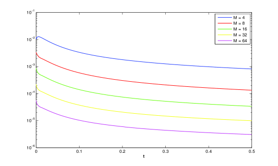
Figure 1: The error $|\|u_{h}^{n}-u(t_{n})\||$ as a function of $t_{n}$ for Example 1.

In Examples 1-3, we choose $\gamma=1.6$ and refine the time steps so that the spatial errors are dominant. We evaluate the exact solution $u$ of problem (1) by truncating the Fourier series in (40) after $60$ terms.

Example 1. Choose $u_{0}(x,y)=xy(1-x)(1-y)$. The Fourier sine coefficients are:

$$(u_{0},\phi_{mn})=8(1-(-1)^{m})(1-(-1)^{n})(mn\pi^{2})^{-3},\quad{\rm for}~{}~{}m,n=1,\,2,\ldots.$$

The initial data $u_{0}\in\dot{H}^{2}(\Omega)\cap L^{\infty}(\Omega).$ Thus, by Theorem 5.3 ($\delta=2$), for each time step $t_{n}$, we expect convergence rate of order $h^{2}\ell_{h}^{5/2}t_{n}^{-\alpha/2}$ in the $L^{\infty}(\Omega)$-norm. Figure 1 shows how the error varies with $t$ for a sequence of solutions obtained by successively doubling the spatial mesh elements, using a log scale. (The same time mesh with $N=1000$ subintervals was used in all cases). In Table 1, we listed the time-space maximum error and its associated convergence rate ($CR$), where second order optimal convergence rates was observed (ignoring the logarithmic factors). So, the influence of the coefficient $t_{n}^{-\alpha/2}=t_{n}^{-3/8}$ is absent. This is probably due to the fact the $u_{0}$ belongs to the smoother space ${\mathcal{C}}^{2}(\overline{\Omega})\cap{\mathcal{C}}_{0}(\overline{\Omega})$, where an $O(h^{2}\ell_{h}^{2})$ rate of convergence is expected, (MT2010b, , Theorem 4.2).

$M$	$\mu=0$		$\mu=0.25$		$\mu=0.5$		$\mu=75$
4	3.008e-02		9.521e-03		3.610e-03		1.597e-03
8	1.054e-02	1.513	1.412e-03	2.754	5.342e-04	2.757	2.401e-04	2.734
16	5.441e-03	0.954	4.112e-04	1.779	1.279e-04	2.062	5.678e-05	2.080
32	1.876e-03	1.536	1.391e-04	1.564	3.344e-05	1.936	1.513e-05	1.908
64	8.667e-04	1.114	6.425e-05	1.114	8.598e-06	1.959	4.055e-06	1.900

Table 2: The weighted error $E_{\mu}$ and the convergence rates, as the number of spatial mesh elements increases, for different choices of the power exponent $\mu$. In each case, we use $1300$ time subintervals.

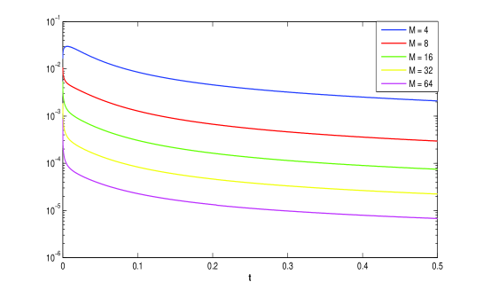
Figure 2: The error $|\|u_{h}^{n}-u(t_{n})\||$ as a function of $t_{n}$ for Example 2.

$M$	$\mu=0$		$\mu=0.5$		$\mu=0.75$		$\mu=1$
8	9.7501e-01		8.545e-03		2.245e-03		1.525e-03
16	7.0054e-01	0.4769	3.852e-03	1.150	6.809e-04	1.721	4.783e-04	1.672
32	3.2311e-01	1.1164	1.776e-03	1.117	2.000e-04	1.767	1.442e-04	1.730
64	1.5301e-01	1.0783	8.409e-04	1.078	6.234e-05	1.682	4.945e-05	1.544

Table 3: The weighted error $E_{\mu}$ and the convergence rates, as the number of spatial mesh elements increases, for different choices of the power weight exponent $\mu$. In each case, we use $1300$ time subintervals.

Example 2. Choose $u_{0}(x,y)=g(x)g(y)$ where $g(z)=z$ on $[0,1/2)$ while $g(z)=1-z$ on $(1/2,1]$, which is less smooth, then the considered $u_{0}$ in the previous example. One can verify that $u_{0}$ has the Fourier sine coefficients $(u_{0},\phi_{mn})=2(1-(-1)^{m})(1-(-1)^{n})(mn\pi^{2})^{-2}(-1)^{mn}$ for $m,n=1,\,2,\ldots.$ The function $u_{0}\in\dot{H}^{1+\epsilon}(\Omega)$ for $0\leq\epsilon<1/2$. So, by Theorem 5.3 ($\delta<1.5$), for each $t_{n}$, we expect $O(h^{2}\ell_{h}^{5/2})t_{n}^{-3\alpha/4}$ convergence rates in the $L^{\infty}(\Omega)$-norm. As in Figure 1, Figure 2 shows how the error varies with $t$ for a sequence of solutions obtained by doubling the spatial mesh elements. (The time mesh with $N=1300$ subintervals was used in all cases). Table 2 provides an alternative view of this data, listing the time-space maximum weighted error $E_{\mu}:=\max_{n=1}^{N}t_{n}^{\mu}|\|u_{h}^{n}-u(t_{n})\||$ and its associated convergence rate $CR$. As expected, ignoring the logarithmic factors, the convergence rate is $2$ when $\mu\geq 3\alpha/4\approx 0.56$, but the rate deteriorates for smaller values of $\mu$ (relatively far from $3\alpha/4$).

Example 3. Choose $u_{0}(x,y)=1$, and so $u_{0}$ has the Fourier sine coefficients $(u_{0},\phi_{mn})=2(1-(-1)^{m})(1-(-1)^{n})(mn\pi^{2})^{-1}$ for $m,n=1,\,2,\ldots.$ The initial data function $u_{0}\in\dot{H}^{\epsilon}(\Omega)\cap L^{\infty}(\Omega)$ for $0\leq\epsilon<1/2$. As in the previous example, Figure 3 shows a consistent decaying in the errors by doubling the number of spatial mesh elements. Another observation is the large impact of the very limited regularity of $u_{0}$ on the errors near $t=0$ in this example. For better justifications of this, see Table 3 where the difference between the maximum error $E_{0}$ and the weighted error $E_{1}$ is very substantial, we also observed very good improvements in the convergence rates $CR$, but not yet optimal due to the time discretization.

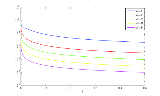
Figure 3: The error $|\|u_{h}^{n}-u(t_{n})\||$ as a function of $t_{n}$ for Example 3.

References

- (1) S. Agmon, A. Douglis, and L. Nirenberg, Estimates near the boundary for solutions of elliptic partial differential equations satisfying general boundary conditions, Comm. Pure. Appl. Math., 12 (1959), 623–727.
- (2) B. Cockburn and K. Mustapha, A hybridizable discontinuous Galerkin method for fractional diffusion problems, Numer. Math., 130 (2015) 293–314.
- (3) C. M. Chen, F. Liu, V. Anh and I. Turner, Numerical methods for solving a two-dimensional variable-order anomalous sub-diffusion equation, Math. Comput., 81 (2012), 345–366.
- (4) E. Cuesta, C. Lubich and C. Palencia, Convolution quadrature time discretization of fractional diffusive-wave equations, Math. Comput., 75 (2006), 673–696.
- (5) M. Cui, Compact alternating direction implicit method for two-dimensional time fractional diffusion equation, J. Comput. Phys., 231 (2012), 2621–2633.
- (6) D. Goswami and A. K. Pani, An alternate approach to optimal -error analysis of semidiscrete Galerkin methods for linear parabolic problems with nonsmooth initial data, Numer. Funct. Anal. Optim., 32 (2011), 946–982.
- (7) B. Jin, R. Lazarov and Z. Zhou, Error estimates for a semidiscrete finite element method for fractional order parabolic equations, SIAM J. Numer. Anal., 51 (2013), 445-–466.
- (8) B. Jin, R. Lazarov, J. Pascal and Z. Zhou, Error analysis of semidiscrete finite element methods for inhomogeneous time-fractional diffusion, IMA J. Numer. Anal., 35 (2015), 561–-582.
- (9) S. Karaa, K. Mustapha and A. K. Pani, Finite volume element method for two-dimensional fractional subdiffusion problems, IMA J. Numer. Anal., 37 (2017), 945–964.
- (10) M. Křìžek and P. Neittaanmäki, On a global superconvergence of the gradient of linear triangular elements, J. Comput. Appl. Math. 18 (1987), 221–-233.
- (11) W. McLean, Regularity of solutions to a time-fractional diffusion equation, ANZIAM J., 52 (2010), 123–138.
- (12) W. McLean, Fast summation by interval clustering for an evolution equation with memory, SIAM J. Sci. Comput., 34 (2012), 3039–3056.
- (13) W. McLean and K. Mustapha, Time-stepping error bounds for fractional diffusion problems with non-smooth initial data, J. Comput. Phys., 293 (2015), 201–217.
- (14) W. McLean and V. Thomée, Numerical solution via Laplace transforms of a fractional order evolution equation, J. Integral Equations Appl., 22 (2010), 57-–94.
- (15) W. McLean and V. Thomée, Maximum-norm error analysis of a numerical solution via Laplace transformation and quadrature of a fractional order evolution equation, IMA J. Numer. Anal., 30 (2010), 208–230.
- (16) K. Mustapha, An implicit finite difference time-stepping method for a sub-diffusion equation, with spatial discretization by finite elements, IMA J. Numer. Anal., 31 (2011), 719–739.
- (17) K. Mustapha and W. McLean, Piecewise-linear, discontinuous Galerkin method for a fractional diffusion equation, Numer. Algor., 56 (2011), 159–184.
- (18) K. Mustapha and D. Schötzau, Well-posedness of version discontinuous Galerkin methods for fractional diffusion wave equations, IMA J. Numer. Anal., 34 (2014), 1226–1246.
- (19) J. Ren and Z. Z. Sun, Numerical algorithm with high spatial accuracy for the fractional diffusion-wave equation with Neumann boundary conditions, J. Sci. Comput., 56 (2013), 381–408.
- (20) V. Thomée. Galerkin finite element methods for parabolic problems, Springer, Second edition, 2006.
- (21) Y. N. Zhang and Z. Z. Sun, Alternating direction implicit schemes for the two-dimensional fractional sub-diffusion equation, J. Comput. Phys., 230 (2011), 8713–8728.