Mean curvature flow with free boundary in embedded cylinders or cones and uniqueness results for minimal hypersurfaces

Abstract.

In this paper we study the mean curvature flow of embedded disks with free boundary on an embedded cylinder or generalised cone of revolution, called the support hypersurface. We determine regions of the interior of the support hypersurface such that initial data is driven to a curvature singularity in finite time or exists for all time and converges to a minimal disk. We further classify the type of the singularity. We additionally present applications of these results to the uniqueness problem for minimal hypersurfaces with free boundary on such suppport hypersurfaces; the results obtained this way do not require a-priori any symmetry or topological restrictions.

1. Introduction

Minimal surfaces and the mean curvature flow in the free boundary setting are natural extrinsic geometric elliptic and parabolic problems that have appeared sporadically throughout the literature for some time (see Nitsche [25, 38], Hildebrandt, Dierkes and collaborators [11, 12, 13] for historical remarks). Inspired by work on the closed hypersurfaces by Huisken [26] and on the Ricci flow by Hamilton [24], Stahl in 1994 made a fundamental contribution [43], establishing local and global existence plus blowup results. Since this time, work has greatly intensified.

We say that a smooth one-parameter family of immersed disks $F:D^{n}\times[0,T)\rightarrow\mathbb{R}^{n+1}$ evolves by the mean curvature flow with free boundary on a support hypersurface $F_{\Sigma}:\Sigma\rightarrow\mathbb{R}^{n+1}$ if

$$\frac{\partial F}{\partial t}=\vec{H}=-H\nu\quad\quad \text{ on }D^{n}\times[0,T)$$

(1) $$\left<\nu,\nu_{\Sigma}\right>=0\quad\quad\quad\quad \text{ on }\partial D^{n}\times[0,T)\,,$$

$$F(\partial D^{n},t)\subset F_{\Sigma}(\Sigma)\,,\quad\text{and} \quad F(\cdot,0)=F_{0}(\cdot)\,.$$

Local existence follows, as demonstrated by Stahl [43], by writing the evolving hypersurfaces as graphs for a short time over their initial data. Stahl additionally gave continuation criteria: a-priori bounds on the second fundamental form are sufficient for the global existence of a solution [45, 44]. In this work he also showed that initially convex data remains convex when the support hypersurface is umbilic, and that in this situation the flow contracts to a round hemishperical point (a Type I singularity). A generalisation to other contact angles of Stahl’s continuation criteria was later obtained by Freire [20].

Buckland studied a setting similar to that of Stahl, and focused on obtaining a classification of singularities according to topology and type [4]. Koeller has generalised the regularity theory developed by Ecker and Huisken [14, 15, 16] to the setting of free boundaries [29]. His main regularity theorem is a criterion under which the singular set will has measure zero.

The author has studied initially graphical mean curvature flow with free boundary, obtaining long time existence results and results on the formation of curvature singularities on the free boundary [50, 48, 49]. A similar angle approach has been employed by Lambert [32] in his work. Edelen’s work is the first systematic treatment of Type II singularities [17]. Convexity estimates play a fundamental role in his work.

Regular solutions of the mean curvature flow with bounded initial area converge as $t\rightarrow\infty$ to minimal hypersurfaces. This also occurs in the setting of free boundary, so it is natural to consider the mean curvature flow as a tool to study minimal surfaces.

Minimal surfaces (and hypersurfaces) are a classical topic in mathematics and as such have received enormous attention in the literature. A review is well beyond the scope of this paper. See for example [39, 21, 40, 41, 33, 5, 6, 8, 9, 37, 2] and the references within. The studies are extensive and from many perspectives: harmonic analysis, geometry, calculus of variations and isoperimetry, complex analysis, partial differential equations, spectral theory, and more.

Work in the free boundary setting is also abundant, see for example [18, 19, 10, 28, 25, 22] and the references therein. Nevertheless there remain many fundamental open questions, in particular to do with the classification and uniqueness of minimal surfaces with free boundary.

Uniqueness for surfaces of prescribed mean curvature has been previously treated by Vogel in [46] under certain conditions. Minimal surfaces and capillarity surfaces of constant mean curvature in right solid cylinders and cones have been studied before by Choe–Park, Lopez–Pyo in [7, 35, 36] via geometric and eliptic techniques. The authors have many results in these papers and others, involving constant mean curvature surfaces with free boundary that invite flow applications. We hope that we are able to inspire progress in this direction.

In this paper we apply the mean curvature flow with free boundary to prove a result in this direction (Theorem 3.1).

In particular, we prove uniqueness and non-existence results for minimal hypersurfaces supported on oscillating or pinching cylinders (embedded double cones) in Euclidean space. There are no dimension, topological, or symmetry restrictions on our results. For example, we prove:

Theorem.

The only bounded smooth immersed minimal hypersurface with free boundary on a catenoid is the flat disk supported at the origin.

Theorem.

There does not exist any bounded smooth immersed minimal hypersurface with free boundary on a cone.

This paper is organised as follows. In Section 2 we study the mean curvature flow and prove our main result that classifies the asymptotic behaviour of initially graphical rotationally symmetric data by properties of the support hypersurface $\Sigma$. When singularities develop, we additionally present some classification of their type. We apply this in Section 3 to prove classification results for immersed minimal hypersurfaces with free boundary.

2. Mean curvature flow with free boundary supported on an oscillating cylinder

The behaviour of immersions flowing by the mean curvature flow with free boundary is largely unknown, with available results in the literature indicating that a complete picture of asymptotic behaviour irrespective of initial condition is extremely difficult to obtain [45, 29]. Therefore the relevant question is: under which initial conditions is it possible to obtain a complete picture of asymptotic behaviour?

Working in the class of graphical hypersurfaces is a viable strategy, so long as the graph condition can be preserved [47, 49, 48, 31]. In each of these works, global results were enabled by symmetry of the initial data and/or of the boundary. Without such symmetries, recent work indicates that graphicality is not in general preserved [3] (even in the case where $F_{\Sigma}(\Sigma)$ is a standard round sphere).

Let us formally set the support hypersurface $F_{\Sigma}:\Sigma\rightarrow\mathbb{R}^{n+1}$ to be rotationally symmetric and generated by the graph of a function $\omega_{\Sigma}:Oz\rightarrow\mathbb{R}$ over the $Oz$ axis. We term such a support hypersurface an oscillating cylinder.

By convention we let $x=(x_{1},\ldots,x_{n})$ be a point in $\mathbb{R}^{n}\subset\mathbb{R}^{n+1}$, with $n\geq 2$ and denote by $y=|x|$ the length of $x$. With this convention the profile curve of the support surface lies in a plane generated by $Oy$ and $Oz$ axes.

We write the graph condition on $\omega_{\Sigma}$ as

(2) $$\left<{\nu}_{\Sigma}(z),e_{1}\right>\ >\ C_{\Sigma}\geq 0,$$

where $C_{\Sigma}$ is a global constant, ${\nu}_{\Sigma}$ the normal to ${\omega}_{\Sigma}$, and $\left<\cdot,\cdot\right>$ is the standard inner product in ${\mathbb{R}}^{n+1}$. Our convention is that $\nu_{\Sigma}$ points away from the interior of the evolving hypersurface.

Let us now describe how a rotationally symmetric graphical mean curvature flow with free boundary $F:D^{n}\times[0,T)\rightarrow\mathbb{R}^{n+1}$ satisfying (1) can be represented by the evolution of a scalar function (the graph function). Let us set $D(t)=(0,r(t))\subset\mathbb{R}$. The Neumann boundary is at $\partial D(t)=r(t)$. The left-hand endpoint of $D(t)$, the zero, is not a true boundary point. It arises from the fact that the scalar generates a radially symmetric graph that is topologically a disk. The coordinate system degenerates at the origin and so it is artificially introduced as a boundary point. This is however a technicality, and no issues arise in dealing with quantities at this fake boundary point, since by symmetry and smoothness we have that the radially symmetric graph is horizontal at the origin.

We represent the mean curvature flow of a radially symmetric graph $F:D^{n}\times[0,T)\rightarrow\mathbb{R}^{n+1}$ by the evolution of its graph function $\omega:D(t)\times[0,T)\rightarrow\mathbb{R}$, that must satisfy the following:

(3) $$\frac{\partial\omega}{\partial t}\ \ =\frac{d^{2}\omega}{dy^{2}}\ \frac{1}{1+(\frac{d\omega}{dy})^{2}}+\frac{d\omega}{dy}\ \frac{n-1}{y} ~{}~{}\text{ on }~{}~{}(0,r(t))\times[0,T),$$

$$\left<{\nu}_{\omega},{\nu}_{\Sigma}\right> =0\text{ and }r(t)={\omega}_{\Sigma}(\omega(r(t),t)) ~{}~{}\text{ on }~{}~{}r(t)\times[0,T),$$

$$\lim_{y\rightarrow 0}\frac{1}{y} \frac{d\omega}{dy}(y)\text{ exists, and }$$

$$\omega(y,0) =\omega_{0} ~{}~{}\text{ on }~{}~{}(0,r(0)).$$

where $\omega_{0}:(0,r(0))\rightarrow\mathbb{R}$ generates the initial graph, $\omega_{0}\in C^{2}((0,r(0)))$, that also satisfies the boundary Neumann boundary condition $\left<{\nu}_{\omega_{0}},{\nu}_{\Sigma}\right>=0$ at $r(0)$.

Note that in this representation the graph direction for $\omega_{\Sigma}$ is perpendicular to the graph direction for $\omega$. (Contrast with [50].) The two graphs share the same axis of revolution. Examples of this include graphs evolving inside a vertical catenoid neck or inside the hole of a vertical unduloid.

2.1. Existence

We prove global existence of solutions to (3) by obtaining uniform $C^{1}$ estimates. The problem (3) is a quasilinear second-order PDE on a time-dependent domain with a Neumann boundary condition. The change in domain can be calculated (see (9)) and depends only on $\omega_{\Sigma}$, $\omega^{\prime}$, and $\omega^{\prime\prime}$. The local unique existence of a solution in this setting is standard and has been discussed in detail in [47, 50].

We note that the uniqueness of a solution shows that the representation (3) of a solution to (1) is preserved.

Our first main result is the following.

Theorem 2.1 (Long time existence).

Let $\omega_{\Sigma}$ and ${\omega}_{0}$ be defined as above. Assume (2), and that

(4) $$\text{there is no point $z^{*}$ where $\omega_{\Sigma}(z^{*})=0$}\,.$$

We further assume for negative and positive infinity that either one of

(5) the limit $$\lim_{z\rightarrow\pm\infty}\omega_{\Sigma}(z)$$ does not exist

or

(6) $$\text{ there exists an $|\alpha|>0$ such that }z\frac{d\omega_{\Sigma}}{dz}(z)>0\text{ for all }\begin{cases}z>\alpha,\text{if }\alpha>0,\\ z<\alpha,\text{if }\alpha<0,\end{cases}$$

hold. Then there exists a global smooth solution $\omega:D(t)\times[0,T)\rightarrow\mathbb{R}$ to the problem (3) that converges smoothly to $\omega_{\infty}:D(\infty)\rightarrow\mathbb{R}$. The function $\omega_{\infty}$ is smooth and generates a minimal surface.

Remark.

The class of support hypersurfaces that satisfy (6) above at both positive and negative infinity are those whose derivative is monotone outside a compact subset with the correct sign. Examples of such include the catenoid.

The catenoid also satisfies condition (5). An example that satisfies (6) but not (5) is

$$\omega_{\Sigma}(z)=2-e^{-z^{2}}\,.$$

More generally, any $\omega_{\Sigma}$ whose derivative is monotone increasing outside a compact set and converges at infinity satisfies (6) but not (5).

Examples that satisfies (5) but not (6) include the unduloids. Examples that satisfy (5) for $z\rightarrow\infty$ and (6) for $z\rightarrow-\infty$ can be pasted together using those mentioned above; for example, mollify the positive part of a catenoid with the negative part of $z\mapsto 2-e^{-z^{2}}$.

Remark.

The condition (4) prevents $\omega_{\Sigma}$ from pinching on the axis of rotation. If this condition is violated, we expect that some solutions to (3) develop finite-time singularities. This case is treated in detailed in subsection 2.3. At such points we do not require that $\omega_{\Sigma}$ is smooth; that is, we allow cones.

Remark.

The condition (6) prevents the solution from shrinking and sliding off to infinity. This would happen for a solution supported in the $\Sigma$ generated by $\omega_{\Sigma}(z)=1+e^{-z^{2}}$. Clearly for such solutions we can not expect convergence.

For the proof, we use standard machinery of parabolic theory (see for example [34, 30]) and its variants for time-dependent domains as discussed in [50, 47]. In these references a maximum principle is proved; we will apply this without further reference.

The condition $\left<{\nu}_{\omega},{\nu}_{\Sigma}\right>=0$ can be written in a simpler way if we take into account the fact that we are working with two graph functions. The outer normal to $\omega$ is given by

$${\nu}_{\omega}=\frac{1}{\sqrt{1+(\frac{d\omega}{dy})^{2}}}\big{(}-\frac{d\omega}{dy},1\big{)}\,.$$

For the unit normal to $\omega_{\Sigma}$ we need to rotate and translate the axes. We find

$${\nu}_{\Sigma}=\frac{1}{\sqrt{1+(\frac{d{\omega}_{\Sigma}}{dz})^{2}}}\big{(}1,-\frac{d{\omega}_{\Sigma}}{dz}\big{)}\,.$$

This transforms the Neumann boundary condition into

(7) $$\frac{d\omega}{dy}(r(t),t)=-\frac{d{\omega}_{\Sigma}}{dz}(\omega(r(t),t))~{}~{}\text{ for all }t\in[0,T),$$

and gives us the following uniform boundary gradient estimate for $\omega$.

Lemma 2.2 (Uniform boundary gradient estimates).

Let $\omega_{\Sigma}$ and ${\omega}_{0}$ be defined as above. Assume (2). Then

$$\bigg{|}\frac{d\omega}{dy}(r(t),t)\bigg{|}\ \leq\ \sqrt{\frac{1}{C_{\Sigma}}-1}$$

for all $t\in[0,T)$.

Proof.

The Neumann condition (7) gives a bound on the gradient of $\omega$ in terms of the gradient $\omega_{\Sigma}$, however the constant is not particularly clear. To find this constant we once more look at the boundary condition. Due to the rotational symmetry we see that the unit normal of $\Sigma$ is, on the boundary, the same vector as the tangent vector to the evolving graphs. Thus

$$\nu_{\Sigma}(\omega(r(t),t))\ =\ \frac{1}{\sqrt{1+(\frac{d\omega}{dy}(r(t),t))^{2}}}\bigg{(}1,\ \frac{d\omega}{dy}(r(t),t)\bigg{)},$$

for all $t\in[0,T)$. Replacing this into the graph condition (2) we find

$$\left<\frac{1}{\sqrt{1+(\frac{d\omega}{dy}(r(t),t))^{2}}}\bigg{(}1,\ \frac{d\omega}{dy}(r(t),t)\bigg{)},e_{1}\right>\ \geq\ C_{\Sigma}.$$

Simplifying we obtain

$$\sqrt{1+\bigg{(}\frac{d\omega}{dy}(r(t))\bigg{)}^{2}}\ \leq\ \frac{1}{C_{\Sigma}},$$

which yields the desired estimate. ∎

Proof of Theorem 2.1.

As we allow the boundary to possibly oscillate, height bounds are not immediate. The maximum principle applies to $|\omega|$, yielding that $|\omega|$ is bounded by the maximum of its boundary and initial values. The main task is to control the value of $|\omega|$ on the Neumann boundary.

For the Hopf lemma to work in excluding new maxima on the Neumann boundary we need to have a certain sign on the directional derivative $\frac{d\omega}{dy}(r(t),t)$. This is not possible since this quantity changes sign with the gradient of the $\Sigma$. This is evident from (7).

To obtain height bounds we proceed as follows. First suppose that there exist two points $z_{sup}$ and $z_{inf}$ such that we have

$$z_{inf}\ <\ \min_{[0,r(0)]}\omega_{0}<\ \max_{[0,r(0)]}\omega_{0}\ <z_{sup}$$

and

$$\frac{d\omega_{\Sigma}}{dz}(z_{sup})=\frac{d\omega_{\Sigma}}{dz}(z_{inf})=0\,.$$

Then the initial graph is contained in

$$\Omega=\{(x,z)\,:\,z\in(z_{inf},z_{sup}),\quad|x|<\omega_{\Sigma}(z)\}\,.$$

The set $\Omega$ is bounded by the support hypersurface and a minimal disk at each end. These act as barriers for the flow: by the avoidance principle we find

$$z_{inf}<\omega<z_{sup}\,.$$

If such points $z_{inf}$ and $z_{sup}$ do not exist, then there do not exist flat disks supported on $\Sigma$ disjoint from the initial graph $\omega_{0}$ that can be used as barriers.

Assume that there is no such disk in

$$U=U^{+}\cup U^{-}$$

where

$$U^{+}=\{(x,z)\,:\,z\geq 0,\,z>\max_{[0,r(0)]}\omega_{0}\text{ or }z<\min_{[0,r(0)]}\omega_{0}\}$$

and

$$U^{-}=\{(x,z)\,:\,z<0,\,z>\max_{[0,r(0)]}\omega_{0}\text{ or }z<\min_{[0,r(0)]}\omega_{0}\}.$$

Each of $U^{+}$ and $U^{-}$ have at most two components, one finite and bounded by the plane $z=0$ and another unbounded. Let $z$ be in the unbounded component of $U^{+}$. There are two cases.

Case 1. Condition (6) is satisfied on an unbounded component $U^{++}$ of $U^{+}$. On this component, the derivative $\frac{d\omega_{\Sigma}}{dz}$ has a sign. As we know that for sufficiently large $z$, the derivative $\frac{d\omega_{\Sigma}}{dz}(z)$ is positive, in this case it must be positive on all of $U^{++}$. Now the boundary condition (7) implies that

$$\frac{d\omega}{dy}(z)<0\,.$$

The Hopf lemma implies that $\omega$ may never reach such a region.

Similarly, if condition (6) is satisfied on an unbounded component $U^{--}$ of $U^{-}$, and $z$ is in the unbounded component of $U^{-}$, then on this component $\frac{d\omega_{\Sigma}}{dz}$ has a sign, and as we know that for sufficiently large $z$ the derivative $\frac{d\omega_{\Sigma}}{dz}(z)$ is negative, in this case it must be negative on all of $U^{--}$. Now the boundary condition (7) implies that for all such $z$

$$\frac{d\omega}{dy}(z)>0\,.$$

The Hopf lemma again implies that $\omega$ may never reach such a region.

Case 2. Condition (5) is satisfied on an unbounded component $U^{++}$ of $U^{+}$. As no minimal disk exists on this component, the derivative $\frac{d\omega_{\Sigma}}{dz}$ again has a sign. If the sign is positive, then the Hopf lemma applies as in Case 1 above. If the sign is negative, then as $z\rightarrow\infty$, the function $\omega_{\Sigma}$ is uniformly bounded from below (by the no pinching condition (4)) and decreasing. Therefore it converges, violating (5).

If condition (5) is satisfied on an unbounded component $U^{--}$ of $U^{-}$ then the derivative is negative. If it were positive, then similarly as above this is in contradiction with (5).

Therefore in either case the evolving surfaces are contained within a compact region of $\mathbb{R}^{n+1}$, and so the graph function $\omega$ is uniformly bounded.

Thus we are left with obtaining gradient estimates for the evolving graphs $\omega:D(t)\times[0,T)\rightarrow\mathbb{R}$.

Let us set $M_{t}:=F(D^{n},t)$. Following [15] we consider the quantity $v=\left<{\nu}_{M_{t}},e_{n+1}\right>^{-1}$, which is modulo a tangential diffeomorphism equal to $\sqrt{1+(\frac{d\omega}{dy})^{2}}$. The function $v$ satisfies

$$\Big{(}\frac{d}{dt}-\Delta_{M_{t}}\Big{)}v\leq 0$$

and this allows us to apply the maximum principle. Since the problem deals with evolving hypersurfaces with boundary we have that the maximum of the gradient is controlled by the maximum between the initial values and the boundary values. In the graphical setting, this translates to the following estimate:

$$\sup_{(0,r(t))}\bigg{|}\frac{d\omega}{dy}\bigg{|}\leq\max\bigg{\{}\sup_{(0,r(0))}\bigg{|}\frac{d\omega}{dy}\bigg{|},\ \sup_{s\in[0,t]}\bigg{|}\frac{d\omega_{0}}{dy}(r(s),s)\bigg{|},\ \ \sup_{s\in[0,t]}\bigg{|}\frac{d\omega}{dy}(0,s)\bigg{|}\bigg{\}}\,,$$

for all $t\in[0,T]$.

We now refine this by considering maxima at the boundary. At the artificial boundary point ($y=0$) the gradient function vanishes due to rotational symmetry; that is,

$$\frac{d\omega}{dy}(0,t)=0\,.$$

Lemma 2.2 gives a uniform estimate for the gradient on the Neumann boundary. We can therefore conclude that

$$\sup_{(0,r(t))}\bigg{|}\frac{d\omega}{dy}\bigg{|}\leq\max\bigg{\{}\sup_{(0,r(0))}\bigg{|}\frac{d\omega_{0}}{dy}\bigg{|},\ \sqrt{\frac{1}{C_{\Sigma}}-1}\bigg{\}}\,.$$

Having obtained a-priori uniform $C^{1}$ estimates for $\omega:D(t)\times[0,T)\rightarrow\mathbb{R}$, the quasilinear parabolic operator (3) may be considered to be linear with bounded coefficients, and for such a problem global existence is standard. Convergence to minimal hypersurfaces is guaranteed by bounded initial area: We calculate

$$\frac{d}{dt}\int_{D^{n}}\,d\mu=-\int_{D^{n}}|H|^{2}d\mu$$

which implies

$$\int_{0}^{\infty}\int_{D^{n}}H^{2}d\mu\,dt\leq\int_{D^{n}}\,d\mu\bigg{|}_{t=0}=c\,.$$

Finally, we have $|D(t)|\geq\inf\omega_{\Sigma}>0$ by assumption, so that $\omega$ does not vanish (c.f. Theorem 2.11). Since all derivatives are uniformly bounded, we may apply a compactness theorem to conclude that $M_{t}\rightarrow M_{\infty}$ and that the mean curvature of $M_{\infty}$ is identically zero. This argument has been used before by many authors, see for example [27, 4, 47]. ∎

Remark.

On the free Neumann boundary, the rotational symmetry of the solution prevents tilt behaviour. This occurs when the normal to the graph becomes parallel to the vector field of rotation for $\Sigma$. This behaviour is explained in much greater detail in [47] and it is present in many situation of free boundary problems [3], thus the need to use the rotationally symmetry in constructing the barriers needed to show the elliptic results.

2.2. Convergence

After showing that the solution to the problem (3) exists for all times we are interested in studying the precise shape that it attains in the limit as $t\rightarrow\infty$, knowing already that it is a minimal hypersurface. In fact, the theory of minimal hypersurfaces (note that the boundary of this disk is a circle) implies that the limit is a flat disk. However, we may prove this directly without requiring the general theory, and so we contribute a proof here. We also give some related results of interest.

Theorem 2.3 (Convergence to flat disks).

Under the hypotheses of Theorem 2.1, the global smooth solution $\omega:D(t)\times[0,\infty)\rightarrow\mathbb{R}$ to the problem (3) satisfyies

$$\displaystyle\lim_{t\rightarrow\infty}\sup_{[0,r(t)]}\bigg{|}\frac{d\omega}{dy}(r(t),t)\bigg{|}=0\,,$$

that is, the solution converges to a flat disk as $t\rightarrow\infty$.

Proof.

First we prove that the gradient on the boundary vanishes.

Let us denote by $u(x)=\omega_{\infty}(|x|)$, $u:D_{\infty}\rightarrow\mathbb{R}$, $D_{\infty}=\{x\in\mathbb{R}^{n}\ :\ y=|x|\in Dom(\omega_{\infty})\}$. The mean curvature of $u$ is

$$H=-div\bigg{(}\frac{\text{D}u}{\sqrt{1+|\text{D}u|^{2}}}\bigg{)}$$

where D and $div$ are the gradient and divergence in $\mathbb{R}^{n}$ respectively. We can then compute using divergence theorem and denoting by $\nu_{\partial D_{\infty}}$ the outer pointing normal to the boundary of the domain $D_{\infty}$:

$$0\ =\ -\int_{D_{\infty}}H\,dx=\int_{D_{\infty}}div\bigg{(}\frac{\text{D}u}{\sqrt{1+|\text{D}u|^{2}}}\bigg{)}\,dx$$

$$\ =\ \int_{\partial D_{\infty}}\frac{\text{D}u}{\sqrt{1+|\text{D}u|^{2}}}\cdot\nu_{\partial D_{\infty}}\,dSx$$

$$\ =\ \int_{\partial D_{\infty}}\frac{\frac{d\omega_{\infty}}{dy}}{\sqrt{1+|\frac{d\omega_{\infty}}{dy}|^{2}}}\,dx$$

$$\ =\ 2\pi r(\infty)\frac{\frac{d\omega_{\infty}}{dy}}{\sqrt{1+|\frac{d\omega_{\infty}}{dy}|^{2}}}(r(\infty))$$

where smoothness of the solution at the rotation axis (i.e. $\frac{d\omega_{\infty}}{dy}(0)=0$) ensures that the second boundary term vanishes. This implies that $\frac{d\omega_{\infty}}{dy}(r(\infty))\equiv 0$.

Using this we can show that the gradient of $\omega_{\Sigma}$ vanishes everywhere:

$$0\ =\ -\int_{D_{\infty}}Hu\,dx=\int_{D_{\infty}}div\bigg{(}\frac{\text{D}u}{\sqrt{1+|\text{D}u|^{2}}}\bigg{)}u\,dx$$

$$\ =\ -\int_{D_{\infty}}\frac{|\text{D}u|^{2}}{\sqrt{1+|\text{D}u|^{2}}}\,dx+\int_{\partial D_{\infty}}\frac{\text{D}u}{\sqrt{1+|\text{D}u|^{2}}}\cdot\nu_{\partial D_{\infty}}u\,dSx$$

$$\ =\ -\int_{D_{\infty}}\frac{|\text{D}u|^{2}}{\sqrt{1+|\text{D}u|^{2}}}\,dx$$

where we have used $\frac{d\omega_{\infty}}{dy}(r(\infty))=0$ for the Neumann boundary and also the smoothness of the solution at the rotation axis, $\frac{d\omega_{\infty}}{dy}(0)=0$ to make the boundary term vanish. This implies that $\text{D}u\equiv 0$ and thus $\frac{d\omega_{\infty}}{dy}\equiv 0$, that is, $\omega_{\infty}$ is a constant. ∎

The above calculation implies the following result, which is interesting in its own right.

Lemma 2.4.

Suppose $F:D^{n}\rightarrow\mathbb{R}^{n+1}$ is an embedded minimal disk with boundary on an oscillating cylinder $\Sigma$ with axis of revolution $Oz$. If

• $F(\partial D)$ is a circle in a plane orthogonal to $Oz$; and

• $F$ is graphical over a disk orthogonal to $Oz$ (but not necessarily rotationally symmetric),

then $F(D^{n})$ is a standard flat disk.

This implies that on the boundary, the gradient of limiting hypersurface will vanish independent of the angle imposed by the flow problem. This explains the non-compactness of the flow (and consequent appearance of translators) in cases where the support hypersurface doesn’t allow this to happen. (See [1, 42, 23] for further results on flows with various contact angles.)

Corollary 2.5.

Suppose $F:D^{n}\times[0,T)\rightarrow\mathbb{R}^{n+1}$ is as in Lemma 2.4, except that at the free boundary where the prescribed angle is $\alpha$, that is,

$$\left<\nu_{\omega},\nu_{\Sigma}\right>=\cos\alpha\,.$$

If there exists no point $z\in Oz$ such that

$$\frac{\frac{d\omega_{\Sigma}}{dz}}{\sqrt{1+\left(\frac{d\omega_{\Sigma}}{dz}\right)^{2}}}=-\cos\alpha$$

then the flow never reaches an equilibrium.

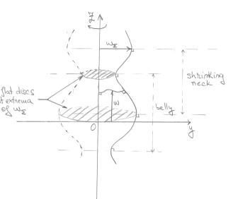
Figure 1. Flat discs at extrema of $\Sigma$.

The graphs generating the contact hypersurface $\Sigma$ are in general oscillating, forming local minima and maxima as they stretch in both directions of the axis $Oz$. The flow may in general converge to any flat disk supported at a critical point of $\omega_{\Sigma}$. Note that the case of $\Sigma$ being a cylinder has been treated previously in [27].

Generically, one expects the flow to converge to minimal disks with the smallest possible area. Such disks are found at local minima of $\omega_{\Sigma}$; however, it appears difficult to rule out convergence to other minimal disks for arbitrary data. In the following we give sufficient conditions on the initial data (that $\Omega$ is contained in a shrinking neck region, see Definition 2.6) to guarantee convergence to a minimal disk supported on a local minimum of $\omega_{\Sigma}$.

Definition 2.6 (Bellies and necks, see Figure 1).

Let $\Sigma$ be an oscillating cylinder. A region of $\Sigma$ is any set ($z_{1},z_{2}\in[-\infty,\infty]$)

$$\Theta(z_{1},z_{2})=\{(x,z)\,:\,|x|<\omega_{\Sigma}(z),\,z\in(z_{1},z_{2})\}\,.$$

A shrinking neck region of $\Sigma$ is any region $\Theta(z_{1},z_{2})$ where for all $z\in(z_{1},z_{2})$

$$\frac{d\omega_{\Sigma}}{dz}(z)=0\quad\Longrightarrow\quad\text{$\omega_{\Sigma}(z)$ is a weak local minimum value for $\omega_{\Sigma}$}\,.$$

A belly region of $\Sigma$ is any region $\Theta(z_{1},z_{2})$ where for all $z\in(z_{1},z_{2})$

$$\frac{d\omega_{\Sigma}}{dz}(z)=0\quad\Longrightarrow\quad\text{$\omega_{\Sigma}(z)$ is a weak local maximum value for $\omega_{\Sigma}$}\,.$$

Theorem 2.7 (Convergence in shrinking necks).

Assume the hypotheses of Theorem 2.1. Suppose that the initial data $F_{0}(D^{n})$ is contained in a shrinking neck region $\Theta(z_{1},z_{2})$. Then the global solution $F:D^{n}\times[0,\infty)\rightarrow\mathbb{R}^{n+1}$ to (1) converges to a flat disk supported at a local minimum of $\omega_{\Sigma}$ in $\Theta(z_{1},z_{2})$. If there is just one such minimum at $z^{*}\in(z_{1},z_{2})$ then the flat disk supported at $\omega_{\Sigma}(z^{*})$ is the unique limit of all solutions to (3) with initial data in $\Theta(z_{1},z_{2})$.

Proof.

Theorems 2.1 and 2.3 yield that the solution exists for all time and converges to a flat disk. It remains to identify which disks may serve as limits for the flow.

All minimal disks in a shrinking neck region are located at local minima of $\omega_{\Sigma}$ by definition. Therefore we will be finished if we can prove that there exists a shrinking neck region $\Theta(w_{1},w_{2})$ such that for all $(x,t)\in D^{n}\times[0,\infty)$,

(8) $$F(D^{n},t)\subset\Theta(w_{1},w_{2})\,.$$

We extend the given shrinking neck region in either direction until we reach a critical point of $\omega_{\Sigma}$. More precisely, let us take

$$w_{1}=\sup\bigg{(}\bigg{\{}z\in(-\infty,z_{1}]\,:\,\frac{d\omega_{\Sigma}}{dz}(z)=0\bigg{\}}\cup\big{\{}-\infty\big{\}}\bigg{)}$$

and

$$w_{2}=\inf\bigg{(}\bigg{\{}z\in[z_{2},\infty)\,:\,\frac{d\omega_{\Sigma}}{dz}(z)=0\bigg{\}}\cup\big{\{}\infty\big{\}}\bigg{)}$$

Clearly $\Theta(z_{1},z_{2})\subset\Theta(w_{1},w_{2})$, and $\Theta(w_{1},w_{2})$ is a region of $\Sigma$. To see that $\Theta(w_{1},w_{2})$ is a shrinking neck region, let $z_{0}\in\Theta(w_{1},w_{2})\setminus\Theta(z_{1},z_{2})$ be a point where

$$\frac{d\omega_{\Sigma}}{dz}(z_{0})=0\text{ and }\text{$\omega_{\Sigma}(z_{0})$ is a local maximum value for $\omega_{\Sigma}$}\,.$$

If $\omega_{\Sigma}^{\prime}(z_{1})=0$ then $w_{1}=z_{1}$; similarly for $z_{2}$. If both conditions are satisfied, then the set $\Theta(w_{1},w_{2})\setminus\Theta(z_{1},z_{2})$ is empty, and such a $z_{0}$ can not exist.

Suppose otherwise. Then either $z_{0}\in(w_{1},z_{1})$ or $z_{0}\in(z_{2},w_{2})$. Suppose the former. Since $\omega_{\Sigma}^{\prime}(z_{0})=0$, $z_{0}\in\{z\in(-\infty,z_{1}]\,:\,\omega_{\Sigma}^{\prime}(z)=0\}$ and $z_{0}>w_{1}$. This contradicts the definition of $w_{1}$. Similarly, $z_{0}\in(z_{2},w_{2})$ contradicts the definition of $w_{2}$. Therefore such a $z_{0}$ can not exist.

We now claim (8). Let us prove this by contradiction. Suppose there exists a sequence of points in space-time $((x_{n},z_{n}),t_{n})\in F(D^{n},t_{n})\times[0,\infty)$ such that $z_{n}\rightarrow z_{\infty}$ such that $z_{\infty}\leq w_{1}$ or $z_{\infty}\geq w_{2}$. Let us first bring $z_{\infty}\leq w_{1}$ to a contradiction.

If $z_{\infty}=-\infty$, this contradicts the height bound from Theorem 2.1. Therefore the only way for $z_{n}\rightarrow z_{\infty}$ such that $z_{\infty}\leq w_{1}$ is if $w_{1}$ is finite. Then by definition of $w_{1}$ we have $\frac{d\omega_{\Sigma}}{dz}(w_{1})=0$ and so there exists a minimal disk supported at $w_{1}$ that serves as a barrier for the solution. Therefore we are left with the case where $z_{\infty}=w_{1}$. In this case, we have for sufficiently large $n$

$$\frac{d\omega_{\Sigma}}{dz}(z_{n})<0\,.$$

(The strict sign follows from the definition of $w_{1}$ and the use of the flat disk as a barrier.) The boundary condition then yields $\frac{d\omega}{dz}(r(t_{n}),t_{n})>0$. Therefore there is no maximum for $\omega(\cdot,t_{n})$ at it’s Neumann boundary. However, by assumption, the graphs $\omega(\cdot,t_{n})$ are moving downward to the flat disk. Therefore there must be a new minimum for $\omega(\cdot,t_{n})$, or equivalently, a new maximum for $|\omega(\cdot,t_{n})|^{2}$. This maximum must be either at the axis of rotation ($y=0$) or in $(0,r(t_{n}))$. The parabolic evolution equation for $\omega$ implies that

$$\sup_{(0,r(t))}\big{|}\omega\big{|}^{2}\leq\max\bigg{\{}\sup_{(0,r(0))}\big{|}\omega\big{|}^{2},\ \sup_{s\in[0,t]}\big{|}\omega(r(s),s)\big{|}^{2},\ \ \sup_{s\in[0,t]}\big{|}\omega(0,s)\big{|}^{2}\bigg{\}}\,.$$

We already ruled out new maxima on the Neumann boundary. The Hopf Lemma implies that new maxima are also impossible at the axis of rotation, since there $\frac{d\omega}{dz}=0$ by symmetry. The only case remaining is that the new maxima occur on the interior, which is clearly a contradiction.

Therefore $z_{\infty}>w_{1}$. A similar argument shows that $z_{\infty}<w_{2}$, and so the claim (8) is proved.

∎

Remark ($\Sigma$ catenoid).

If $\Sigma$ is a catenoid or it has only one global minimum then $\Theta(-\infty,\infty)$ is a shrinking neck region. Theorem 2.7 above then yields that solutions converge as $t\rightarrow\infty$ to the unique flat disk perpendicular to $\Sigma$ at this point (c.f. the analogous result in [50]).

If the initial data is contained in a maximal finite belly region, then it is trapped in this region, by comparison with flat disks at either end (c.f. the proof of Theorem 2.7 above). If the initial data is to one side of the highest (or lowest) flat disk in the belly region, then it is also in a shrinking neck region, and the previous theorem applies. If the initial data intersects any flat disk in the belly region, then the asymptotic behaviour of the flow becomes more complicated. In the following result we give a sufficient conditions that guarantees the flow (even if initially in a belly region intersecting a flat disk) moves out of the belly region and converges to a flat disk in a shrinking neck region.

Figure 2. Uniqueness of limiting disks for flows with initial data contained in a shrinking neck region.

Theorem 2.8 (Convergence for initial data in bellies).

Assume the hypotheses of Theorem 2.1. Suppose that the initial data $F_{0}(D^{n})$ is contained in a belly region $\Theta(z_{1},z_{2})$ such that it intersects a flat disk in $\Theta(z_{1},z_{2})$ and:

1. $H(\cdot,0)<0$ and $\omega_{0}(r(0))>\alpha$ where $\alpha$ is the $z$-coordinate of the highest minimal disk in $\Theta(z_{1},z_{2})$; or

2. $H(\cdot,0)>0$ and $\omega_{0}(r(0))<\beta$ where $\beta$ is the $z$-coordinate of the lowest minimal disk in $\Theta(z_{1},z_{2})$.

Then the global solution $F:D^{n}\times[0,\infty)\rightarrow\mathbb{R}^{n+1}$ to (1) converges to a flat disk supported at a local minimum of $\omega_{\Sigma}$ in a shrinking neck region. If $\Theta(z_{1},z_{2})\subset\Theta(z_{min},z_{max})$ where $\Theta(z_{min},z_{max})$ is a maximal belly region and $-\infty<z_{min}<z_{max}<\infty$ then the flat disk supported at $\omega_{\Sigma}(z_{max})$ is the unique limit of all solutions to (3) with initial data satisfying (a) and the flat disk supported at $\omega_{\Sigma}(z_{min})$ is the unique limit of all solutions to (3) with initial data satisfying (b).

Remark.

A sign on the mean curvature does not imply that the profile $\omega$ is convex or concave. Note that if $\alpha=\beta$ then we set $z^{*}=\alpha=\beta$ (see Figure 3).

If the belly region is infinite on either side, then we do not expect solutions to converge. This is not possible here, as it would contradict the assumptions of Theorem 2.1.

Before we start the proof of the theorem we require a result on preservation of the sign of the mean curvature for mean curvature flow with free boundary. This is due to Stahl [43].

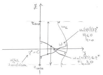
Figure 3. Uniqueness of flat disks in belly regions

Proposition 2.9 ([43]).

Let $H(\cdot,0)\geq(\leq)\,0$ everywhere on $M_{0}$. Then $H(\cdot,t)\geq(\leq)\,0$ for all $t\geq 0$ where $M_{t}$ a solution of the mean curvature flow with free boundary.

For completeness we sketch the proof. It is based on the use of the maximum principle and the fact that on the boundary the directional derivative of the mean curvature is equal to the mean curvature multiplied by a component of the second fundamental form of $\Sigma$ at that point. The Hopf Lemma then yields a contradiction, for any smooth $\Sigma$, with the appearance of a new zero (maximum or minimum) on the boundary. The strong maximum principle yields the strict sign for all strictly positive times.

Proof of Theorem 2.8.

Theorems 2.1 and 2.3 yield that the solution exists for all time and converges to a flat disk. Suppose we are in situation (a). First we translate the $Oy$ axis so that $\alpha=0$, and $z_{1}\leq 0\leq z_{2}$. After this translation, the definition of belly region implies

$$z\frac{d\omega_{\Sigma}}{dz}\ \leq\ 0,$$

for all $z\in\Theta(z_{1},z_{2})$. As in the proof of Theorem 2.7, consider the maximal belly region $\Theta(z_{min},z_{max})\supset\Theta(z_{1},z_{2})$. By assumption, neither of $z_{1}$, $z_{2}$ may be infinite, and so by definition of $z_{min}$, $z_{max}$, there exist flat disks on the boundary of $\Theta(z_{min},z_{max})$ supported on $\Sigma$.

We are in the case of negative mean curvature. To show that the graphs will ascend and converge as $t\rightarrow\infty$ to the flat disk at $z=z_{max}$ we look at the derivative of the boundary point $r(t)$. Since

$$r(t)\ =\ \omega_{\Sigma}(\omega(r(t),t))\,,$$

we calculate

(9) $$r^{\prime}(t)=\frac{d\omega_{\Sigma}}{dz}\bigg{(}\frac{\partial\omega}{\partial t}+\frac{d\omega}{dy}r^{\prime}(t)\bigg{)}\,.$$

Substituting in the boundary condition (7) and $\frac{\partial\omega}{\partial t}=-Hv$ yields

$$r^{\prime}(t)\ =\ -\frac{H}{v}\frac{d\omega_{\Sigma}}{dz},$$

where we have once again denoted $v=\sqrt{1+(\frac{d\omega}{dy})^{2}}=\sqrt{1+(\frac{d\omega_{\Sigma}}{dz})^{2}}>0$ at the boundary points. Now for all $z\geq 0$ (recall the translation)

$$\frac{d\omega_{\Sigma}}{dz}\leq 0.$$

This gives us that $r^{\prime}(t)<0$ which means that $r(t)$ is decreasing. As we are in a belly region above the highest flat disk, this implies that $\omega(r(t),t)$ is monotone increasing. Given that the graphs exist for all times and converge to a flat disk, the first such encountered by the solution is the flat disk at $z_{max}$. Since this disk also serves as a barrier for the solution, the proof is finished. ∎

Remark (Height restrictions on the boundary point).

If $\alpha=\beta=z^{*}$, the restriction on $\omega_{0}(r(0))\geq z^{*}$ is necessary.

This is because otherwise the mean curvature of $\omega_{0}$ can not be everywhere negative. If $\omega_{0}(r(0))<z^{*}$, then $\omega_{0}$ would have to turn after passing the translated $Oy$ axis so that it reaches the axis of rotation orthogonally, creating a mean convex region. To see this note that by (7), for all $z<z^{*}$ we have $\frac{d\omega_{0}}{dy}(r(0))\ <\ 0$. At the rotation axis the gradient is vanishing by smoothness, that is, $\frac{d\omega_{0}}{dy}(0)=0$. This implies that there exits a point $y^{*}\in(0,r(0)]$ such that $\frac{d^{2}\omega_{0}}{dy^{2}}(y^{*})<0$. Otherwise the gradient would just increase, giving a contradiction. At this point we calculate the mean curvature:

$$0>H=-\frac{\frac{d^{2}\omega_{0}}{dy^{2}}}{\sqrt{1+(\frac{d\omega_{0}}{dy})^{2}}^{3}}-\frac{n-1}{y{\sqrt{1+(\frac{d\omega_{0}}{dy})^{2}}}}\frac{d\omega_{0}}{dy}$$

and obtain that $\frac{d\omega_{0}}{dy}(y^{*})>0$. Since $\frac{d\omega_{0}}{dy}(r(0))<0$, we see that there exists a point $y_{2}\in(0,r(0)]$ such that $\frac{d\omega_{0}}{dy}(y_{2})=0$. Repeating the above by replacing the point at zero with $y_{2}$, we find a second point $y_{3}\in(y_{2},r(0)]$ with the property that the gradient vanishes at $y_{2}$. Denote by $y_{1}=0$. In this way we obtain a sequence of points converging $y_{k}\rightarrow y_{\infty}$ as $k\rightarrow\infty$, such that $\frac{d\omega_{0}}{dy}(y_{k})=0$. If $y_{\infty}=r(0)$, then by smoothness of $\omega_{0}$ we obtain a contradiction with the strict sign by the Neumann condition (7). If $y_{\infty}\in(0,r(0))$ then by smoothness of $\omega_{0}$, in a left-neighbourhood of $y_{\infty}$ we have that $\omega_{0}$ is flat. This implies in particular that the first two derivatives of $\omega_{0}$ vanish there, and so the mean curvature vanishes also. This is in contradiction with $H<0$.

Remark (Initial boundary point at $z^{*}$).

If the initial data has Neumann boundary tangential to the flat disk at $z^{*}$, and is disjoint from the flat disk in the interior, it will immediately move into a shrinking neck region and Theorem 2.7 applies. If it is not immediately disjoint from the flat disk, then it is either tangential or crosses the flat disk. If tangential, then the mean curvature is zero at some interior points, and this is a contradiction with the mean curvature having a definite sign. If it crosses the disk, then the same proof in the above remark applies to show that the mean curvature must change sign.

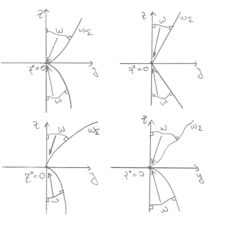
Figure 4. Examples of finite-time singularities.

2.3. Singularities

In this section we treat the case when the support hypersurface $\Sigma$ pinches on its axis of rotation; that is, there exists one or more points $z^{*}$ such that $\omega_{\Sigma}(z^{*})=0$. We do not require that $\Sigma$ is smooth at those points so examples of such support hypersurfaces include cones, parabolae or hypersurfaces that form cusps at the rotation axis.

Definition 2.10.

Let $\omega_{\Sigma}:Oz\rightarrow[0,\infty)$ be a continuous function. Assume that $\omega_{\Sigma}$ is smooth outside finitely many points $P=\{w_{1},\ldots,w_{n_{p}}\}$, where $\omega_{\Sigma}(w_{i})=0$; that is, $\omega_{\Sigma}\in C^{\infty}_{loc}(Oz\setminus P)$. Assume that there exists a compact set $K\supset P$ such that

$$z\frac{d\omega_{\Sigma}}{dz}(z)>0\quad\text{ for all }z\in\mathbb{R}\setminus K\,.$$

The function $\omega_{\Sigma}$ generates a smooth rotationally symmetric disconnected hypersurface $F_{\Sigma}:\Sigma\rightarrow\mathbb{R}^{n+1}$, where $\Sigma$ is the disjoint union of $n_{p}+1$ cylinders. We term the support hypersurface $F_{\Sigma}$ a pinching cylinder.

Note that if $n_{p}=0$ in Definition 2.10 we are in one of the cases considered earlier in the paper.

Remark.

Although we require that $\omega_{\Sigma}$ be only continuous on $\mathbb{R}$, it may pinch and be smooth (or analytic) everywhere on $\mathbb{R}$. For example, this is the case if $\omega_{\Sigma}$ is a non-negative polynomial in $z$ with zeros; for example,

$$\omega_{\Sigma}(z)=(z-2)^{2}(z+2)^{2}\,.$$

Theorem 2.11 (Flow in conical pinching cylinders).

Let $\Sigma$ be a pinching cylinder as in Definition 2.10 with $n_{p}=1$. Let $w_{1}=z^{*}=0$. Assume (2) (understood as limits from the left and right at points in $P$). Suppose that for all $z\in\mathbb{R}\setminus\{0\}$,

(10) $$z\frac{d\omega_{\Sigma}}{dz}(z)>0\,.$$

Then the maximal time of existence for any solution $\omega:D(t)\times[0,T)\rightarrow\mathbb{R}$ to (3) satisfies $T<\infty$. The hypersurfaces $F:D^{n}\times[0,T)\rightarrow\mathbb{R}^{n+1}$ generated by $\omega$ contract as $t\rightarrow T$ to the point $(0,z^{*})$.

Proof.

The proof height and gradient estimates goes through exactly as in Theorem 2.1 and Lemma 2.2. We do not have global existence however, as in this setting, we do not have a uniform bound on $r(t)$ from below. We claim that the solution $\omega:D(t)\times[0,T)\rightarrow\mathbb{R}$ of (3) exists smoothly for all $t\in[0,T)$, $T<\infty$, and $r(t)\rightarrow 0$ as $t\rightarrow 0$.

To see this, we first show $T<\infty$. For the sake of contradiction, assume that the graphs exist for all time, that is, $T=\infty$. Then the solutions converge to a flat disck perpendicular to the contact hypersurface $\Sigma$ as per Theorem (2.3). However, any flat disk must be supported on $\Sigma$ by a point where the gradient of $\omega_{\Sigma}$ vanishes. Such a point (by (10)) does not exist.

Therefore $T<\infty$. Since the height and gradient bounds provides us with uniform $C^{1}$ estimates for all time, the only posibility preventing global existence is that $r(t)\rightarrow 0$ as $t\rightarrow T$. Therefore the solution converges to a point on the axis of rotation. The solution however must also satisfy the Neumann condition, and so the limit point must be a point where $\Sigma$ pinches off; as there is only one such point where this occurs, we are done. ∎

Remark (Non-rotational initial data).

Any initially bounded mean curvature flow with free boundary, irrespective of symmetry or topological properties, exists at most for finite time when supported on a pinching cylinder as in Theorem 2.11. This is because so long as the initial immersion is bounded, we may always construct a rotationally symmetric graphical solution such that the initial immersion lies between this solution and the pinchoff point $(0,z^{*})$. The flow generated by this pair of initial data remain disjoint by the comparison principle, and as the rotationally symmetric solution contracts to a point in finite time, the flow of immersions must either develop a curvature singularity in finite time or contract to the same point (and possibly remain regular while doing so).

Similarly, in a shrinking neck region, we may use the rotationally symmetric graphical solutions as barriers to obtain that any mean curvature flow with free boundary whose initial data is contained in a shrinking neck either exists for all time and converges to a flat disk or develops a curvature singularity in finite time.

Our next task is to determine the type of the singularity. We are able to show that in most cases the singularity is Type I or better (Type 0: that it is not a curvature singularity at all but a loss of domain). The cases that allow us to do this are when the gradient of $\omega_{\Sigma}$ is bounded. This includes cones and cusps. We are not yet able to conclude the same for the case of parabolae, that is, when the gradient of $\omega_{\Sigma}$ is unbounded on $Oz\setminus P$.

Definition 2.12 (Singularities).

Let $F:D^{n}\times[0,T)\rightarrow\mathbb{R}^{n+1}$ be a mean curvature flow with free boundary supported on a pinching cylinder. If there exists an $\varepsilon>0$ such that for all $t\in(T-\varepsilon,T)$

• the second fundamental form is uniformly bounded, that is,

  $$|A|^{2}(x,t)\leq C<\infty\,,$$

  then we say the singularity is Type 0;

• the second fundamental form is uniformly controlled under parabolic rescaling, that is,

  $$|A|^{2}(x,t)\leq\frac{C}{T-t}\,,$$

  then we say the singularity is Type I;

• neither of the previous two cases apply, we say the singularity is Type II.

Theorem 2.13 (Type 1 singularities).

Let $\omega_{\Sigma}$ and $\omega_{0}$ be as in Theorem 2.11. If there exist two constants $0<C_{1}<\infty$ and $C_{2}<\infty$ such that for $z$ sufficiently close to $z^{*}$ we have:

• Conical pinchoff

  $$C_{1}\leq\bigg{|}\frac{d\omega_{\Sigma}}{dz}(z^{*})\bigg{|}\leq C_{2},$$

  then the singularity from Theorem 2.11 is Type I;

• Polynomial pinchoff

  $$C_{1}|\omega_{\Sigma}(z)|^{\sigma}\leq\bigg{|}\frac{d\omega_{\Sigma}}{dz}(z)\bigg{|}\leq C_{2}|\omega_{\Sigma}(z)|^{\sigma}\,,$$

  for $\sigma<1$, then the singularity from Theorem 2.11 is Type I, and in particular there exist $\hat{C}_{1},\hat{C}_{2}$ such that for $t$ sufficiently close to $T$ we have

  $$\frac{\hat{C}_{1}}{T-t}\leq|A|^{2}(x,t)\leq\frac{\hat{C}_{2}}{T-t}$$

Before starting the proof of the theorem we need to compute the norm squared of the second fundamental form and mean curvature in terms of the profile curve $\omega$.

Lemma 2.14.

For a rotationally symmetric hypersurface generated by the rotation of a graph function $\omega$ about an axis perpendicular to the graph direction, the norm squared of the second fundamental form and mean curvature are given by the formulae

$$|A|^{2} =\frac{1}{(1+(\frac{d\omega}{dy})^{2})^{3}}\Big{(}\frac{d^{2}\omega}{dy^{2}}\Big{)}^{2}+\frac{1}{1+(\frac{d\omega}{dy})^{2}}\frac{1}{y^{2}}\Big{(}\frac{d\omega}{dy}\Big{)}^{2}$$

$$H =-\frac{1}{\sqrt{1+(\frac{d\omega}{dy})^{2}}^{3}}\frac{d^{2}\omega}{dy^{2}}\ -\ \frac{1}{\sqrt{1+(\frac{d\omega}{dy})^{2}}}\frac{1}{y}\frac{d\omega}{dy}.$$

Proof.

The proof is a lengthy but straightforward computation using the parametrisation for a rotationally symmetric graph, that is, $F(x,t)=(x,\omega(|x|,t))$, where $x\in D^{n}$, and denoting $y=|x|$. ∎

Proof of Theorem 2.13.

Given that the gradient of $\omega_{\Sigma}$ is uniformly bounded, as before in the proof of Theorem 2.1 and the proof of Theorem 2.11 we have that the $\omega$ satisfy uniform $C^{1}$ estimates up to the time of singularity. Let us denote this time by $T$. The estimates imply that there exists a constant $C_{4}<\infty$ depending only on the initial data such that

$$\bigg{|}\frac{d^{2}\omega}{dy^{2}}\bigg{|}\leq C_{4}\,.$$

Thus the second fundamental form will explode at worst as quickly as $r(t)\searrow 0$, that is, there exists a constant $C=C(C_{2},C_{4})<\infty$ such that

$$|A|^{2}(y,t)\leq C\frac{1}{y^{2}}\bigg{(}\frac{d\omega}{dy}\bigg{)}^{2}(y,t),$$

for all $t$ and $y$.

On the rotation boundary, that is at $y=0$, the right hand side is uniformly bounded by symmetry. (A unique tangent plane exists at the origin.) Everywhere else the gradient and $1/y$ is bounded by an absolute constant multiplied by it’s value at the boundary.

Thus there exists a constant denoted by abuse of notation $C=C(C,C_{2},C_{4})<\infty$ such that

(11) $$\sup_{[0,r(t)]}|A|^{2}(t)\ \leq\ C\frac{1}{r(t)^{2}}\bigg{(}\frac{d\omega}{dy}\bigg{)}^{2}(r(t),t)\,,$$

for all $t$. From here we separate the proof into the two cases. First assume the case of cones, that is there exists a second constant $C_{1}>0$ such that

$$\bigg{|}\frac{d\omega_{\Sigma}}{dz}(z^{*})\bigg{|}\geq C_{1}.$$

From our estimates above, there exists a constant denoted by abuse of notation $C=C(C,C_{2},C_{4})<\infty$ such that

(12) $$\sup_{[0,r(t)]}|A|^{2}(t)\ \leq\ C\frac{1}{r(t)^{2}},$$

for all $t$. To compute the rate of blow up for the boundary point $r(t)$, we use the time evolution for $r(t)$ (computed earlier in the proof of Theorem 2.8)

$$r^{\prime}(t)\ =\ -\frac{H}{v}\frac{d\omega_{\Sigma}}{dz}.$$

Substituting for the Neumann boundary condition (7) and the formula for the mean curvature in Lemma 2.14, we obtain

$$r^{\prime}(t)r(t)\ =\ -\frac{(\frac{d\omega}{dy})^{2}}{1+(\frac{d\omega}{dy})^{2}}\ -\ \frac{\frac{d^{2}\omega}{dy^{2}}\frac{d\omega}{dy}}{(1+(\frac{d\omega}{dy})^{2})^{2}}r(t).$$

Given that the gradient is bounded away from $0$ by $C_{1}$ (using the Neumann condition and the bound on the gradient of $\omega_{\Sigma}$), and also bounded from above by $C_{2}$, we have that

$$r^{\prime}(t)r(t)\ \leq\ -\frac{C_{1}^{2}}{1+C_{2}^{2}}\ -\ \frac{\frac{d^{2}\omega}{dy^{2}}\frac{d\omega}{dy}}{(1+(\frac{d\omega}{dy})^{2})^{2}}r(t).$$

We know $r(t)\rightarrow 0$ as $t\rightarrow T$ where $T$ is the final time of existence. We also know that the second derivative is bounded by $C_{4}$. Thus we can choose $0<t^{*}<T$, independently of the sign of the second term above in $r^{\prime}(t)r(t)$, such that

$$r^{\prime}(t)r(t)\ \leq\ -C_{5}.$$

for some constant $0<C_{5}=C_{5}(C_{1},C_{2},C_{4})$ for all $t^{*}<t<T$. Note that $C_{5}$ is bounded away from $0$ is independent of $t$. Integrating from $t<T$ to $T$ and using the fact that $r(T)=0$ we find

$$r^{2}(t)\ \geq\ 2C_{5}(T-t),$$

for all $t\geq t^{*}$. Substituting this into (12) we obtain the following bound for the second fundamental form

$$\sup_{[0,r(t)]}|A|^{2}(t)\ \leq\ \frac{C}{2C_{5}}\frac{1}{T-t}$$

for all $t\in(t^{*},T)$, that is, the singularity is Type I.

Now consider the case of polynomial pinchoff: for $z$ sufficiently close to $z^{*}$ we have

$$C_{1}|\omega_{\Sigma}(z)|^{\sigma}\leq\bigg{|}\frac{d\omega_{\Sigma}}{dz}(z)\bigg{|}\leq C_{2}|\omega_{\Sigma}(z)|^{\sigma}\,.$$

Using $r^{\prime}(t)=-\frac{H}{v}\omega_{\Sigma}^{\prime}(\omega(r(t),t))$ and the above we estimate:

$$r^{1-2\sigma}(t)r^{\prime}(t)\leq Cr^{1-2\sigma}(t)-\frac{C_{1}}{1+C_{2}r^{2\sigma}}\leq-C_{1}/2$$

for $t$ sufficiently close to $T$ (since $\sigma<1$) and some $C=C(C_{1},C_{2},C_{4})$ , and so

$$-r^{2-2\sigma}(t)=\int_{t}^{T}(r^{2-2\sigma}(t))^{\prime}\,ds\leq\int_{t}^{T}-C_{1}(1-\sigma)\,ds=-C_{1}(1-\sigma)(T-t)\,.$$

This implies

$$\frac{1}{r^{2-2\sigma}(t)}\leq\frac{1}{C_{1}(2-2\sigma)}\frac{1}{T-t}\,.$$

Estimating as above (beginning at estimate (11) earlier) we find

$$\sup_{[0,r(t)]}|A|^{2}(t) \leq C\frac{1}{r^{2}(t)}\bigg{(}\frac{d\omega}{dy}\bigg{)}^{2}(r(t),t)$$

$$=C\frac{1}{r^{2}(t)}\bigg{(}\frac{d\omega_{\Sigma}}{dz}\bigg{)}^{2}(\omega(r(t),t))$$

$$\leq C\frac{1}{r^{2-2\sigma}(t)}$$

$$\leq C(\sigma)\frac{1}{T-t}\,.$$

Therefore the singularity is Type I. Now as the assumption is two-sided, we find that (for a different constant $C(\sigma)$) the same estimate above for the second fundamental form holds, but from below. Therefore the singularity is no better and no worse than Type I, and the statement follows.

∎

Remark.

Conical pinchoff is a special case of polynomial pinchoff. For polynomial pinchoff, it isn’t possible to satisfy all condition of the theorem for $\sigma\geq 1$. For $\sigma>0$, the pinchoff is convex and for $\sigma<0$ the pinchoff is concave. These names come from the following examples:

$$\omega_{\Sigma}(z)=z^{\alpha}$$

satisfies $\omega_{\Sigma}^{\prime}(z)=\alpha\omega_{\Sigma}^{1-\frac{1}{\alpha}}(z)$. Therefore $\alpha>1$ corresponds to $\sigma\in(0,1)$ and $\alpha<1$ corresponds to $\sigma<0$. Clearly all asymptotically polynomial pinchoffs are allowed by the condition $\sigma<1$. Concave pinchoff is related to the singularity resulting from mean curvature flow with free boundary supported in the sphere, studied by Stahl [45].

Theorem 2.15 (Type 0 singularities).

Let $\omega_{\Sigma}:Oz\rightarrow\mathbb{R}$ be the profile curve of a rotationally symmetric hypersurface satisfying (2) and

$$\lim_{z\rightarrow\infty}\omega_{\Sigma}(z)=0\,,\quad\bigg{|}\frac{d\omega_{\Sigma}}{dz}(z)\bigg{|}\leq C|\omega_{\Sigma}|^{1+\sigma}(z)\,,\quad\sigma>0\,.$$

Then the maximal time of existence for any solution $\omega:D(t)\times[0,T)\rightarrow\mathbb{R}$ to (3) satisfies $T=\infty$. The hypersurfaces $F:D^{n}\times[0,T)\rightarrow\mathbb{R}^{n+1}$ generated by $\omega$ satisfy

$$||A||_{\infty}^{2}(t)\rightarrow\alpha_{0}\quad\text{as $t\rightarrow\infty$}\,,$$

and so either

• $F(D^{n},t)$ converges smoothly to a flat disk; or

• Modulo translation, $F(D^{n},t)$ converges to a flat point, that is, a singularity of Type 0.

Proof.

First, a uniform a-priori gradient bound follows by applying Lemma 2.2. Note that the difference

$$\sup\{|\omega(y_{1},t)-\omega(y_{2},t)|\,:\,y_{1},y_{2}\in[0,r(t)]\}$$

is uniformly bounded, since if it weren’t, this would contradict the uniform gradient bound. Therefore, the translated flow $\hat{\omega}(y,t):=\omega(y,t)-\omega(0,t)$ has uniformly bounded height, and so, exists for all time. Note importantly that the domain of $\hat{\omega}$ is equal to the domain of $\omega$, that is, $r(t)$ is invariant under translation.

For the original solution, we have $T=\infty$ and global existence, however the height may become unbounded.

We calculate, as in the proof of Theorem 2.13 above,

$$\sup_{[0,r(t)]}|A|^{2}(t) \leq C\frac{1}{r^{2}(t)}\bigg{(}\frac{d\omega}{dy}\bigg{)}^{2}(r(t),t)$$

$$\leq C\frac{1}{r^{2}(t)}\bigg{(}\frac{d\omega_{\Sigma}}{dz}\bigg{)}^{2}(\omega(r(t),t))$$

$$\leq C\frac{|\omega_{\Sigma}|^{2+2\sigma}(r(t),t)}{r^{2}(t)}$$

$$\leq Cr^{2\sigma}(t)\,.$$

Therefore the claim follows with $\displaystyle\alpha_{0}=C\lim_{t\rightarrow\infty}r^{2\sigma}(t)$. If $r(t)\rightarrow 0$ and $|\omega(0,t)|\rightarrow\infty$ then the limit is a flat point, and if $r(t)\rightarrow r_{\infty}>0$ then the proof of Theorem 2.3 applies and the limit is a flat disk. ∎

Remark.

Examples of support hypersurfaces with profile curves satsifying the conditions of Theorem 2.15 include exponentials and reciprocal polynomials, such as

$$\omega_{\Sigma}(z)=e^{-z}$$

and a (monotone) mollification of

$$\omega_{\Sigma}(z)=\begin{cases}\frac{1}{z}\,,\quad\text{for }z>1\\ -z+2\,,\quad\text{for }z\leq 1\,.\end{cases}$$

3. Uniqueness results for minimal hypersurfaces with free boundary

In this section we apply the parabolic results proved earlier to the uniqueness problem for minimal hypersurfaces with free boundary. We emphasize that the results in this section hold for immersed minimal hypersurfaces with free boundary, that is, without any restrictions on topology, symmetry, or graphicality.

In this section we assume $\Sigma$ to be a pinching oscillating cylinder, as in Section 2.3. Examples of this include catenoids, unduloids, cones, parabolae, and so on.

Generically, an oscillating cylinder decomposes into belly regions and shrinking neck regions (if maximal, these have non-trivial overlap). In belly regions, there may exist flat minimal disks that are not rotationally symmetric with respect to the $Oz$ axis; for example, if part of the belly region is spherical, then there exist infinitely many such tilted flat disks. Clearly these disks serve as barriers for the mean curvature flow with free boundary. Unfortunately, there does not exist a mean curvature flow with free boundary that is asymptotic (in positive time) to such slanted disks.

For the case of a shrinking neck region however, solutions are asymptotic to flat disks, and these disks have $Oz$ as their axis of rotation. Our result is the following:

Theorem 3.1 (Uniqueness in shrinking necks).

Let $F:M^{n}\rightarrow\mathbb{R}^{n+1}$ be an immersed bounded smooth minimal hypersurface with free boundary on a pinching cylinder $F_{\Sigma}:\Sigma\rightarrow\mathbb{R}^{n+1}$. If $F(M)\subset\Theta(z_{1},z_{2})$ where $\Theta(z_{1},z_{2})$ is a shrinking neck region, then $F(M)$ is a standard flat disk.

Proof.

We squeeze the minimal hypersurface between two rotationally symmetric graphical solutions to the mean curvature flow with free boundary. First, consider the maximal shrinking neck region $\Theta(z_{min},z_{max})\supset\Theta(z_{1},z_{2})$. Suppose that $\Theta(z_{min},z_{max})$ is bounded. Then by maximality there exists flat minimal disks supported on $F_{\Sigma}$ at $z_{min}$ and $z_{max}$. As $F(M)\subset\Theta(z_{1},z_{2})\subset\Theta(z_{min},z_{max})$, there exist graphical rotationally symmetric smooth hypersurfaces $f^{1},f^{2}:D^{n}\rightarrow\mathbb{R}^{n+1}$ supported on $F_{\Sigma}$ and disjoint from the minimal disks at $z_{min}$, $z_{max}$, and $F(M)$ such that $f^{1}<F(M)<f^{2}$.

Now take $f^{1}$ and $f^{2}$ as initial data for the mean curvature flow with free boundary, generating flows $F^{1},F^{2}:D^{n}\times[0,\infty)\rightarrow\mathbb{R}^{n+1}$. By the results of Section 2, each of these flows converge to minimal disks. By the comparison principle (see for example [43, 47]) we have that the hypersurfaces $F^{1}(D^{n},t)$, $F^{2}(D^{n},t)$ are disjoint from each other, as well as disjoint from $F(M)$. This is because if they were to intersect at any point, it would be a point of tangency, and then, as $F(M)$ is minimal and $F^{i}(D^{n},t)$ is not minimal for all $t\in[0,\infty)$, this would be a contradiction. (This is the only part of the argument where we require any smoothness of the minimal immersion $F$.)

Now the region these flows foliate is

$$\Omega=\bigcup\Big{\{}F^{i}(D^{n},t)\,:\,t\in[0,\infty)\Big{\}}\,.$$

The minimal hypersurface $F(M)$ must be disjoint from this region, and it may not lie above $f^{2}$ or below $f^{1}$ by construction. Therefore, as $F(M)$ lies in a shrinking neck region $\Theta(z_{1},z_{2})$, it is supported in a purely cylindrical portion of $\Theta(z_{1},z_{2})$.

We extend our foliation through this cylindrical region by translation, that is, we take one further flow $g:D^{n}\times[0,1]\rightarrow\mathbb{R}^{n+1}$ where

$$\partial_{t}g=\nu\,,\quad g(D^{n},0)=\lim_{t\rightarrow\infty}F^{1}(D^{n},t)\,,\quad g(D^{n},1)=\lim_{t\rightarrow\infty}F^{2}(D^{n},t)\,.$$

This flow completes the foliation of the region containing $F(M)$. The flow $g$ is a flow of minimal hypersurfaces. Therefore, at a first point and time $t^{*}\in[0,1]$ of tangency, we must have $F(M)=g(D^{n},t^{*})$, that is, $F(M)$ is a flat disk.

Suppose now that $\Theta(z_{min},z_{max})$ is unbounded on one or both sides; say $z_{1}=-\infty$. Now the boundedness hypothesis on $F(M)$ implies that there exists a rotationally symmetric graphical smooth hypersurface $f^{1}:D^{n}\rightarrow\mathbb{R}^{n+1}$ supported on $F_{\Sigma}$ and disjoint from $F(M)$ such that $f^{1}<F(M)$. We can use this as initial data and proceed using the argument above. Similarly, if $z_{2}=\infty$, boundedness of $F(M)$ implies that there exists a rotationally symmetric graphical smooth hypersurface $f^{2}:D^{n}\rightarrow\mathbb{R}^{n+1}$ supported on $F_{\Sigma}$ and disjoint from $F(M)$ such that $F(M)<f^{2}$. Again, we can use this $f^{2}$ in the argument above.

In all cases $F(M)$ is a flat disk, and so we are finished. ∎

This theorem implies in particular:

Corollary 3.2 (Non-existence of immersed minimal free boundary hypersurface with topological type other than that of a disk).

There exists no smooth bounded immersed minimal $n$-dimensional hypersurface supported on $F_{\Sigma}$ in any topology other than that of the flat disk.

Corollary 3.3 (The catenoid case).

The only bounded smooth immersed minimal hypersurface with free boundary on a catenoid is the flat disk supported at the origin.

Similar results are provable using the same method as above. We have not attempted to give an exhaustive list. When there is no minimal disk supported on $F_{\Sigma}$, then one may guess that there is no minimal hypersurface supported on $F_{\Sigma}$. One situation where this holds is the following:

Proposition 3.4 (Non-existence of minimal hypersurfaces in cones, parabolae).

Let $F_{\Sigma}$ be as in Theorem (2.11). There does not exist an immersed bounded smooth minimal hypersurface $F:M^{n}\rightarrow\mathbb{R}^{n+1}$ supported on $F_{\Sigma}$.

Proof.

As the proof is similar to that of Theorem 3.1, we only give a brief outline. In Theorem 2.11, there exists precisely one point of pinching for $F_{\Sigma}$. Without loss of generality we can assume that $F_{\Sigma}$ lies either above or below this point of pinching. In either case, we can construct a rotationally symmetric graphical smooth hypersurface $f:D^{n}\rightarrow\mathbb{R}^{n+1}$ supported on $F_{\Sigma}$ such that $F(M)$ lies between $f$ and the pinching point of $\Sigma$. We use $f$ to generate a mean curvature flow with free boundary. This yields a foliation of the region between $f$ and the pinching point, which must by smoothness have a first point and time of tangency with $F$. However $F$ is minimal and the flow generated by $f$ is not; this yields a contradiction. ∎

References

- [1] S.J. Altschuler and L.F. Wu. Translating surfaces of the non-parametric mean curvature flow with prescribed contact angle. Calc. Var. Partial Differential Equations, 2:101–111, 1994.
- [2] B. Andrews and H. Li. Embedded constant mean curvature tori in the three-sphere. Journal of Differential Geometry, 99(2):169–189, 2015.
- [3] B. Andrews and V.-M. Wheeler. Counterexamples to graph preservation in mean curvature flow with free boundary. preprint, 2016.
- [4] J.A. Buckland. Mean curvature flow with free boundary on smooth hypersurfaces. J. Reine Angew. Math., 586:71–90, 2005.
- [5] J. Choe. The isoperimetric inequality for a minimal surface with radially connected boundary. Annali della Scuola Normale Superiore di Pisa-Classe di Scienze, 17(4):583–593, 1990.
- [6] J. Choe and R. Gulliver. The sharp isoperimetric inequality for minimal surfaces with radially connected boundary in hyperbolic space. Inventiones mathematicae, 109(1):495–503, 1992.
- [7] J. Choe and S.-H. Park. Capillary surfaces in a convex cone. Mathematische Zeitschrift, 267(3-4):875–886, 2011.
- [8] T. H. Colding and W. P. Minicozzi. The space of embedded minimal surfaces of fixed genus in a 3-manifold iv; locally simply connected. Annals of mathematics, 160(2):573–615, 2004.
- [9] T. H. Colding and W. P. Minicozzi. A course in minimal surfaces, volume 121. American Mathematical Soc., 2011.
- [10] R. Courant. Dirichlet’s principle, conformal mapping, and minimal surfaces. Courier Corporation, 2005.
- [11] Ulrich Dierkes, Stefan Hildebrandt, Albrecht Küster, and Ortwin Wohlrab. Minimal surfaces i, volume 295 of grundlehren der mathematischen wissenschaften, 1992.
- [12] Ulrich Dierkes, Stefan Hildebrandt, and Anthony Tromba. Regularity of minimal surfaces, volume 340. Springer Science & Business Media, 2010.
- [13] Ulrich Dierkes, Stefan Hildebrandt, and Anthony J Tromba. Global Analysis of Minimal Surfaces, vol. 341 of Grundlehren der Mathematischen Wissenschaften (Fundamental Principles of Mathematical Sciences). Springer, Heidelberg, 2010.
- [14] K. Ecker. Regularity Theory for Mean Curvature Flow. Birkhauser, 2004.
- [15] K. Ecker and G. Huisken. Mean curvature evolution of entire graphs. Ann. of Math. (2), 130(2):453–471, 1989.
- [16] K. Ecker and G. Huisken. Interior estimates for hypersurfaces moving by mean curvature. Invent. Math., 105(1):547–569, 1991.
- [17] N. Edelen. Convexity estimates for mean curvature flow with free boundary. arXiv preprint arXiv:1411.3864, 2014.
- [18] A. Fraser and R. Schoen. The first steklov eigenvalue, conformal geometry, and minimal surfaces. Advances in Mathematics, 226(5):4011–4030, 2011.
- [19] A. Fraser and R. Schoen. Sharp eigenvalue bounds and minimal surfaces in the ball. Inventiones mathematicae, pages 1–68, 2012.
- [20] A. Freire. Mean curvature motion of graphs with constant contact angle at a free boundary. Analysis & PDE, 3(4):359–407, 2010.
- [21] E. Giusti. Minimal surfaces and functions of bounded variation. Birkhauser, 1984.
- [22] M. Grüter, S. Hildebrandt, and J. CC Nitsche. On the boundary behavior of minimal surfaces with a free boundary which are not minima of the area. manuscripta mathematica, 35(3):387–410, 1981.
- [23] B. Guan. Mean curvature motion of nonparametric hypersurfaces with contact angle condition. Elliptic and parabolic methods in geometry, page 47, 1996.
- [24] R.S. Hamilton. Three-manifolds with positive Ricci curvature. J. Differential Geom., 17:255–306, 1982.
- [25] S. Hildebrandt and J. CC Nitsche. Minimal surfaces with free boundaries. Acta Mathematica, 143(1):251–272, 1979.
- [26] G. Huisken. Flow by mean curvature of convex surfaces into spheres. J. Differential Geom., 20(1):237–266, 1984.
- [27] G. Huisken. Non-parametric mean curvature evolution with boundary conditions. J. Differential Equations, 77:369–378, 1989.
- [28] W. Jäger. Behavior of minimal surfaces with free boundaries. Communications on Pure and Applied Mathematics, 23(5):803–818, 1970.
- [29] A. Koeller. On the Singularity Sets of Minimal Surfaces and a Mean Curvature Flow. PhD thesis, Freie Universität Berlin, 2007.
- [30] O.A. Ladyshenzkaya, V.A. Solonnikov, and N.N. Ural ceva. Linear and quasilinear equations of parabolic type, Translations of Mathematical Monographs, Band 23. Amer. Math. Soc., Rhode Island, 1968.
- [31] B. Lambert. The constant angle problem for mean curvature flow inside rotational tori. arXiv preprint arXiv:1207.4422, 2012.
- [32] B. Lambert. The perpendicular neumann problem for mean curvature flow with a timelike cone boundary condition. Transactions of the American Mathematical Society, 366(7):3373–3388, 2014.
- [33] H. B. Lawson. Complete minimal surfaces in s3. Annals of Mathematics, pages 335–374, 1970.
- [34] G.M. Lieberman. Second order parabolic differential equations. World Scientific Pub. Co. Inc., 1996.
- [35] R. López and J. Pyo. Capillary surfaces in a cone. Journal of Geometry and Physics, 76:256–262, 2014.
- [36] R. López and J. Pyo. Capillary surfaces of constant mean curvature in a right solid cylinder. Mathematische Nachrichten, 287(11-12):1312–1319, 2014.
- [37] J. C.C. Nitsche. On new results in the theory of minimal surfaces. Bulletin of the American Mathematical Society, 71(2):195–270, 1965.
- [38] Johannes-C-C Nitsche and Jerry-M Feinberg. Lectures on minimal surfaces. vol. 1. 1985.
- [39] R. Osserman. A survey of minimal surfaces. Courier Corporation, 2002.
- [40] A. H. Schoen. Infinite periodic minimal surfaces without self-intersections. 1970.
- [41] R. Schoen and S.-T. Yau. Existence of incompressible minimal surfaces and the topology of three dimensional manifolds with non-negative scalar curvature. Annals of Mathematics, 110(1):127–142, 1979.
- [42] L. Shahriyari. Translating graphs by mean curvature flow. PhD thesis, The John Hopkins University, Baltimore, Maryland, USA, 2012.
- [43] A. Stahl. Über den mittleren Krümmungsfluss mit Neumannrandwerten auf glatten Hyperflächen. PhD thesis, Fachbereich Mathematik, Eberhard-Karls-Universität, Tüebingen, Germany, 1994.
- [44] A. Stahl. Convergence of solutions to the mean curvature flow with a neumann boundary condition. Calc. Var. Partial Differential Equations, 4(5):421–441, 1996.
- [45] A. Stahl. Regularity estimates for solutions to the mean curvature flow with a neumann boundary condition. Calc. Var. Partial Differential Equations, 4(4):385–407, 1996.
- [46] T. Vogel. Uniqueness for certain surfaces of prescribed mean curvature. Pacific Journal of Mathematics, 134(1):197–207, 1988.
- [47] V.-M. Vulcanov. Mean curvature flow of graphs with free boundaries. PhD thesis, Freie Universität, Fachbereich Mathematik und Informatik, Berlin, Germany, 2011.
- [48] G. Wheeler and V.-M. Wheeler. Mean curvature flow with free boundary outside a hypersphere. arXiv preprint arXiv:1405.7774, 2014.
- [49] V.-M. Wheeler. Mean curvature flow of entire graphs in a half-space with a free boundary. Journal für die reine und angewandte Mathematik (Crelles Journal), 2014(690):115–131, 2014.
- [50] V.-M. Wheeler. Non-parametric radially symmetric mean curvature flow with a free boundary. Math. Z., 276(1-2):281–298, 2014.