Understanding Convolutional Neural Networks

Abstract

Convoulutional Neural Networks (CNNs) exhibit extraordinary performance on a variety of machine learning tasks. However, their mathematical properties and behavior are quite poorly understood. There is some work, in the form of a framework, for analyzing the operations that they perform. The goal of this project is to present key results from this theory, and provide intuition for why CNNs work.

1 Introduction

1.1 The supervised learning problem

We begin by formalizing the supervised learning problem which CNNs are designed to solve. We will consider both regression and classification, but restrict the label (dependent variable) to be univariate. Let $X\in\mathcal{X}\subset\mathbb{R}^{d}$ and $Y\in\mathcal{Y}\subset\mathbb{R}$ be two random variables. We typically have $Y=f(X)$ for some unknown $f$. Given a sample $\{(x_{i},y_{i})\}_{i=1,\dots,n}$ drawn from the joint distribution of $X$ and $Y$, the goal of supervised learning is to learn a mapping $\hat{f}:\mathcal{X}\to\mathcal{Y}$ which minimizes the expected loss, as defined by a suitable loss function $L:\mathcal{Y}\times\mathcal{Y}\to\mathbb{R}$. However, minimizing over the set of all functions from $\mathcal{X}$ to $\mathcal{Y}$ is ill-posed, so we restrict the space of hypotheses to some set $\mathcal{F}$, and define

$$\hat{f}=\operatorname*{arg\,min}_{f\in\mathcal{F}}\mathrm{E}[L(Y,f(X))]$$ (1)

1.2 Linearization

A common strategy for learning classifiers, and the one employed by kernel methods, is to linearize the variations in $f$ with a feature representation. A feature representation is any transformation of the input variable $X$; a change of variable. Let this transformation be given by $\Phi(X)$. Note that the transformed variable need not have a lower dimension than $X$. We would like to construct a feature representation such that $f$ is linearly separable in the transformed space i.e.

$$f(X)=\langle\Phi(X),w\rangle$$ (2)

for regression, or

$$f(X)=\mathit{sign}(\langle\Phi(X),w\rangle)$$ (3)

for binary classification. Classification algorithms like Support Vector Machines (SVM) [3] use a fixed feature representation that may, for instance, be defined by a kernel.

1.3 Symmetries

The transformation induced by kernel methods do not always linearize $f$ especially in the case of natural image classification. To find suitable feature transformations for natural images, we must consider their invariance properties. Natural images show a wide range of invariances e.g. to pose, lighting, scale. To learn good feature representations, we must suppress these intra-class variations, while at the same time maintaining inter-class variations. This notion is formalized with the concept of symmetries as defined next.

Definition 1 (Global Symmetry)

Let $g$ be an operator from $\mathcal{X}$ to $\mathcal{X}$. $g$ is a global symmetry of $f$ if $f(g.x)=f(x)\ \forall x\in\mathcal{X}$.

Definition 2 (Local Symmetry)

Let $G$ be a group of operators from $\mathcal{X}$ to $\mathcal{X}$ with norm $|.|$. $G$ is a group of local symmetries of $f$ if for each $x\in\mathcal{X}$, there exists some $C_{x}>0$ such that $f(g.x)=f(x)$ for all $g\in G$ such that $|g|<C_{x}$.

Global symmetries rarely exist in real images, so we can try to construct features that linearize $f$ along local symmetries. The symmetries we will consider are translations and diffeomorphisms, which are discussed next.

1.4 Translations and Diffeomorphisms

Given a signal $x$, we can interpolate its dimensions and define $x(u)$ for all $u\in\mathbb{R}^{n}$ ($n=2$ for images). A translation is an operator $g$ given by $g.x(u)=x(u-g)$. A diffeomorphism is a deformation; small diffeomorphisms can be written as $g.x(u)=x(u-g(u))$.

We seek feature transformations $\Phi$ which linearize the action of local translations and diffeomorphisms. This can be expressed in terms of a Lipschitz continuity condition.

$$\|\Phi(g.x)-\Phi(x)\|\leq C|g|\|x\|$$ (4)

1.5 Convolutional Neural Networks

Convolutional Neural Networks (CNNs), introduced by Le Cun et al. [6] are a class of biologically inspired neural networks which solve equation $\eqref{eq:supl}$ by passing $X$ through a series of convolutional filters and simple non-linearities. They have shown remarkable results in a wide variety of machine learning problems [8]. Figure 1 shows a typical CNN architecture.

A convolutional neural network has a hierarchical architecture. Starting from the input signal $x$, each subsequent layer $x_{j}$ is computed as

$$x_{j}=\rho W_{j}x_{j-1}$$ (5)

Here $W_{j}$ is a linear operator and $\rho$ is a non-linearity. Typically, in a CNN, $W_{j}$ is a convolution, and $\rho$ is a rectifier $\max(x,0)$ or sigmoid $\nicefrac{{1}}{{1+\exp(-x)}}$. It is easier to think of the operator $W_{j}$ as a stack of convolutional filters. So the layers are filter maps and each layer can be written as a sum of convolutions of the previous layer.

$$x_{j}(u,k_{j})=\rho\Big{(}\sum_{k}(x_{j-1}(.,k)\ast W_{j,k_{j}}(.,k))(u)\Big{)}$$ (6)

Here $\ast$ is the discrete convolution operator:

$$(f\ast g)(x)=\sum_{u=-\infty}^{\infty}f(u)g(x-u)$$ (7)

The optimization problem defined by a convolutional neural network is highly non-convex. So typically, the weights $W_{j}$ are learned by stochastic gradient descent, using the backpropagation algorithm to compute gradients.

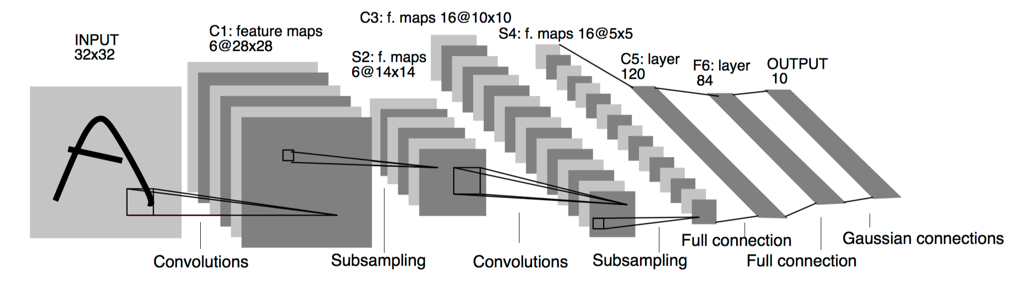
Figure 1: Architecture of a Convolutional Neural Network (from LeCun et al. [7])

1.6 A mathematical framework for CNNs

Mallat [10] introduced a mathematical framework for analyzing the properties of convolutional networks. The theory is based on extensive prior work on wavelet scattering (see for example  [2, 1]) and illustrates that to compute invariants, we must separate variations of $X$ at different scales with a wavelet transform. The theory is a first step towards understanding general classes of CNNs, and this paper presents its key concepts.

2 The need for wavelets

Although the framework based on wavelet transforms is quite successful in analyzing the operations of CNNs, the motivation or need for wavelets is not immediately obvious. So we will first consider the more general problem of signal processing, and study the need for wavelet transforms.

In what follows, we will consider a function $f(t)$ where $t\in\mathbb{R}$ can be considered as representing time, which makes $f$ a time varying function like an audio signal. The concepts, however, extend quite naturally to images as well, when we change $t$ to a two dimensional vector. Given such a signal, we are often interested in studying its variations across time. With the image metaphor, this corresponds to studying the variations in different parts of the image. We will consider a progression of tools for analyzing such variations. Most of the following material is from the book by Gerald [5].

2.1 Fourier transform

The Fourier transform of $f$ is defined as

$$\hat{f}(\omega)\equiv\int_{-\infty}^{\infty}f(t)e^{-2\pi i\omega t}dt$$ (8)

The Fourier transform is a powerful tool which decomposes $f$ into the frequencies that make it up. However, it should be quite clear from equation $\eqref{eq:fourier}$ that it is useless for the task we are interested in. Since the integral is from $-\infty$ to $\infty$, $\hat{f}$ is an average over all time and does not have any local information.

2.2 Windowed Fourier transform

To avoid the loss of information that comes from integrating over all time, we might use a weight function that localizes $f$ in time. Without going into specifics, let us consider some function $g$ supported on $[-T,0]$ and define the windowed Fourier transform (WFT) as

$$\tilde{f}(\omega,t)\equiv\int_{-\infty}^{\infty}f(u)g(u-t)e^{-2\pi i\omega u}du$$ (9)

It should be intuitively clear that the WFT can capture local variations in a time window of width $T$. Further, it can be shown that the WFT also provides accurate information about $f$ in a frequency band of some width $\Omega$. So does the WFT solve our problem? Unfortunately not; and this is a consequence of Theorem 1 which is stated very informally next.

Theorem 1 (Uncertainty Principle)

Let $f$ be a function which is small outside a time-interval of length $T$, and let its Fourier transform be small outside a frequency-band of width $\Omega$. There exists a positive constant $c$ such that

$$\Omega T\geq c$$

Because of the Uncertainty Principle, $T$ and $\Omega$ cannot both be small. Roughly speaking, this implies that the WFT cannot capture small variations in a small time window (or in the case of images, a small patch).

2.3 Continuous wavelet transform

The WFT fails because it introduces scale (the width of the window) into the analysis. The continuous wavelet transform involves scale too, but it considers all possible scalings and avoids the problem faced by the WFT. Again, we begin with a window function $\psi$ (supported on $[-T,0]$), this time called a mother wavelet. For some fixed $p\geq 0$, we define

$$\psi_{s}(u)\equiv|s|^{-p}\psi\Big{(}\frac{u}{s}\Big{)}$$ (10)

The scale $s$ is allowed to be any non-zero real number. With this family of wavelets, we define the continuous wavelet transform (CWT) as

$$\tilde{f}(s,t)\equiv(f\ast\psi_{s})(t)$$ (11)

where $\ast$ is the continuous convolution operator:

$$(p\ast q)(x)\equiv\int_{-\infty}^{\infty}p(u)q(x-u)du$$ (12)

The continuous wavelet transform captures variations in $f$ at a particular scale. It provides the foundation for the operation of CNNs, as will be explored next.

3 Scale separation with wavelets

Having motivated the need for a wavelet transform, we will now construct a feature representation using the wavelet transform. Note that convolutional neural network are covariant to translations because they use convolutions for linear operators. So we will focus on transformations that linearize diffeomorphisms.

Theorem 2

Let $\phi_{J}(u)=2^{-nJ}\phi(2^{-J}u)$ be an averaging kernel with $\int\phi(u)du=1$. Here $n$ is the dimension of the index in $\mathcal{X}$, for example, $n=2$ for images. Let $\{\psi_{k}\}_{k=1}^{K}$ be a set of $K$ wavelets with zero average: $\int\psi_{k}(u)du=0$, and from them define $\psi_{j,k}(u)\equiv 2^{-jn}\psi_{k}(2^{-j}u)$. Let $\Phi_{J}$ be a feature transformation defined as

$$\Phi_{J}x(u,j,k)=|x\ast\psi_{j,k}|\ast\phi_{J}(u)$$

Then $\Phi_{J}$ is locally invariant to translations at scale $2^{J}$, and Lipschitz continuous to the actions of diffemorphisms as defined by equation $\eqref{eq:lips}$ under the following diffeomorphism norm.

$$|g|=2^{-J}\sup_{u\in\mathbb{R}^{n}}|g(u)|+\sup_{u\in\mathbb{R}^{n}}|\nabla g(u)|$$ (13)

Theorem 2 shows that $\Phi_{J}$ satisfies the regularity conditions which we seek. However, it leads to a loss of information due to the averaging with $\phi_{J}$. The lost information is recovered by a hierarchy of wavelet decompositions as discussed next.

4 Scattering Transform

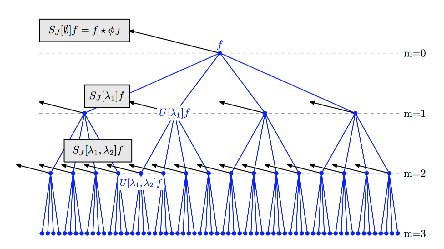
Figure 2: Architecture of the scattering transform (from Estrach [4])

Convolutional Neural Networks transform their input with a series of linear operators and point-wise non-linearities. To study their properties, we first consider a simpler feature transformation, the scattering transform introduced by Mallat [9]. As was discussed in section 1.5, CNNs compute multiple convolutions across channels in each layer; So as a simplification, we consider the transformation obtained by convolving a single channel:

$$x_{j}(u,k_{j})=\rho\Big{(}(x_{j-1}(.,k_{j-1})\ast W_{j,h})(u)\Big{)}$$ (14)

Here $k_{j}=(k_{j-1},h)$ and $h$ controls the hierarchical structure of the transformation. Specifically, we can recursively expand the above equation to write

$$x_{J}(u,k_{J})=\rho(\rho(\dots\rho(x\ast W_{1,h_{1}})\ast\dots)\ast W_{J,h_{J}})$$ (15)

This produces a hierarchical transformation with a tree structure rather than a full network. It is possible to show that the above transformation has an equivalent representation through wavelet filters i.e. there exists a sequence $p\equiv(\lambda_{1},\dots,\lambda_{m})$ such that

$$x_{J}(u,k_{J})=S_{J}[p]x(u)\equiv(U[p]x\ast\phi_{J})(u)\equiv(\rho(\rho(\dots\rho(x\ast\psi_{\lambda_{1}})\ast\dots)\ast\psi_{\lambda_{m}})\ast\phi_{J})(u)$$ (16)

where the $\psi_{\lambda_{i}}$s are suitably choses wavelet filters and $\phi_{J}$ is the averaging filter defined in Theorem 2. This is the wavelet scattering transfom; its structure is similar to that of a convolutional neural network as shown in figure 2, but its filters are defined by fixed wavelet functions instead of being learned from the data. Further, we have the following theorem about the scattering transform.

Theorem 3

Let $S_{J}[p]$ be the scattering transform as defined by equation $\eqref{eqn:scatter}$. Then there exists $C>0$ such that for all diffeomorphisms $g$, and all $L^{2}(\mathbb{R}^{n})$ signals $x$,

$$\|S_{J}[p]g.x-S_{J}[p]x\|\leq Cm|g|\|x\|$$ (17)

with the diffeomorphism norm $|g|$ given by equation $\eqref{eqn:diffnorm}$.

Theorem 3 shows that the scattering transform is Lipschitz continuous to the action of diffemorphisms. So the action of small deformations is linearized over scattering coefficients. Further, because of its structure, it is naturally locally invariant to translations. It has several other desirable properties [4], and can be used to achieve state of the art classification errors on the MNIST digits dataset [2].

5 General Convolutional Neural Network Architectures

The scattering transform described in the previous section provides a simple view of a general convolutional neural netowrk. While it provides intuition behind the working of CNNs, the transformation suffers from high variance and loss of information because we only consider single channel convolutions. To analyze the properties of general CNN architectures, we must allow for channel combinations. Mallat [10] extends previously introduced tools to develop a mathematical framework for this analysis. The theory is, however, out of the scope of this paper. At a high level, the extension is achieved by replacing the requirement of contractions and invariants to translations by contractions along adaptive groups of local symmetries. Further, the wavelets are replaced by adapted filter weights similar to deep learning models.

6 Conclusion

In this paper, we tried to analyze the properties of convolutional neural networks. A simplified model, the scattering transform was introduced as a first step towards understanding CNN operations. We saw that the feature transformation is built on top of wavelet transforms which separate variations at different scales using a wavelet transform. The analysis of general CNN architectures was not considered in this paper, but even this analysis is only a first step towards a full mathematical understanding of convolutional neural networks.

References

- Andén and Mallat [2014] Joakim Andén and Stéphane Mallat. Deep scattering spectrum. Signal Processing, IEEE Transactions on, 62(16):4114–4128, 2014.
- Bruna and Mallat [2013] Joan Bruna and Stéphane Mallat. Invariant scattering convolution networks. Pattern Analysis and Machine Intelligence, IEEE Transactions on, 35(8):1872–1886, 2013.
- Cortes and Vapnik [1995] Corinna Cortes and Vladimir Vapnik. Support-vector networks. Machine learning, 20(3):273–297, 1995.
- [4] Joan Bruna Estrach. Scattering representations for recognition.
- Gerald [1994] Kaiser Gerald. A friendly guide to wavelets, 1994.
- Le Cun et al. [1990] B Boser Le Cun, John S Denker, D Henderson, Richard E Howard, W Hubbard, and Lawrence D Jackel. Handwritten digit recognition with a back-propagation network. In Advances in neural information processing systems. Citeseer, 1990.
- LeCun et al. [1998] Yann LeCun, Léon Bottou, Yoshua Bengio, and Patrick Haffner. Gradient-based learning applied to document recognition. Proceedings of the IEEE, 86(11):2278–2324, 1998.
- LeCun et al. [2015] Yann LeCun, Yoshua Bengio, and Geoffrey Hinton. Deep learning. Nature, 521(7553):436–444, 2015.
- Mallat [2012] Stéphane Mallat. Group invariant scattering. Communications on Pure and Applied Mathematics, 65(10):1331–1398, 2012.
- Mallat [2016] Stéphane Mallat. Understanding deep convolutional networks. arXiv preprint arXiv:1601.04920, 2016.