Particle creation by peak electric field

Abstract

The particle creation by the so-called peak electric field is considered. The latter field is a combination of two exponential parts, one exponentially increasing and another exponentially decreasing. We find exact solutions of the Dirac equation with the field under consideration with appropriate asymptotic conditions and calculate all the characteristics of particle creation effect, in particular, differential mean numbers of created particle, total number of created particles, and the probability for a vacuum to remain a vacuum. Characteristic asymptotic regimes are discussed in detail and a comparison with the pure asymptotically decaying field is considered.

I Introduction

Particle creation from the vacuum by strong external electromagnetic fields was studied already for a long time; see, for example, Refs.  Sch51 ; Nikis70a ; Nikis70b ; Gitman77 ; Gitman77b ; GMR85 ; FGS ; BirDav82 ; Grib ; GelTan15 ; GelTan15b ; GavGT06 ; GavGit15 . To be observable, the effect needs very strong electric fields in magnitudes compared with the Schwinger critical field. Nevertheless, recent progress in laser physics allows one to hope that an experimental observation of the effect can be possible in the near future, see Refs. Dun09 ; Dun09b ; Dun09c ; Dun09d ; Dun09e for the review. Electron-hole pair creation from the vacuum becomes also an observable effect in graphene and similar nanostructures in laboratory; see, e.g., dassarma ; dassarmab . The particle creation from the vacuum by external electric and gravitational backgrounds plays also an important role in cosmology and astrophysics BirDav82 ; Grib ; GelTan15 ; GelTan15b ; AndMot14 .

It should be noted that the particle creation from the vacuum by external fields is a nonperturbative effect and its calculation essentially depends on the structure of the external fields. Sometimes calculations can be done in the framework of the relativistic quantum mechanics, sometimes using semiclassical and numerical methods (see Refs. BirDav82 ; Grib ; GelTan15 ; GelTan15b for the review). In most interesting cases, when the semiclassical approximation is not applicable, the most convincing consideration of the effect is formulated in the framework of quantum field theory, in particular, in the framework of QED, see Ref. Gitman77 ; Gitman77b ; FGS ; GavGT06 ; GavGit15 and is based on the existence of exact solutions of the Dirac equation with the corresponding external field. Until now, only few exactly solvable cases are known for either time-dependent homogeneous or constant inhomogeneous electric fields. One of them is related to the constant uniform electric field Sch51 , another one to the so-called adiabatic electric field $E\left(t\right)=E\cosh^{-2}\left(t/T_{\mathrm{S}}\right)\,$NarNik70 (see also DunHal98 ; GavGit96 ), the case related to the so-called $T$-constant electric field BagGitShv75 ; GavGit96 ; GavGit08 ; GavGit08b , the case related to a periodic alternating electric field NarNIk74 ; NarNIk74b , and several constant inhomogeneous electric fields of the similar forms where the time $t$ is replaced by the spatial coordinate $x$. The existence of exactly solvable cases of particle creation is extremely important both for deep understanding of quantum field theory in general and for studying quantum vacuum effects in the corresponding external fields. In our recent work AdoGavGit14 , we have presented a new exactly solvable case of particle creation in an exponentially decreasing in time electric field.

In the present article, we consider for the first time particle creation in the so-called peak electric field, which is a combination of two exponential parts, one exponentially increasing and the other exponentially decreasing. This is another new exactly solvable case. We demonstrate that in the field under consideration, one can find exact solutions with appropriate asymptotic conditions and perform nonperturbative calculations of all the characteristics of particle creation process. In some respects, the peak electric field shares similar features with the Sauter-like electric field, while in other respects it can be treated as a pulse created by laser beams. Switching the peak field on and off, we can imitate electric fields that are specific to condensed matter physics, in particular to graphene or Weyl semimetals as was reported, e.g., in Refs. lewkowicz10 ; lewkowicz10b ; lewkowicz10c ; Vandecasteele10 ; GavGitY12 ; Zub12 ; KliMos13 ; Fil+McL15 ; VajDorMoe15 .

In our calculations, we use the general theory of Ref. Gitman77 ; Gitman77b ; FGS and follow in the main the consideration of particle creation effect in a homogeneous electric field GavGit96 . To this end we find complete sets of exact solutions of the Dirac and Klein-Gordon equations in the peak electric field and use them to calculate differential mean numbers of created particle, total number of created particles, and the probability for a vacuum to remain a vacuum. Characteristic asymptotic regimes (slowly varying peak field, short pulse field, and the most asymmetric case related to exponentially decaying field) are discussed in detail and a comparison with the pure asymptotically decaying field is considered.

II Peak electric field

II.1 General

In this section we introduce the so-called peak electric field, that is a time-dependent electric field directed along an unique direction

$$\mathbf{E}\left(t\right)=\left(E^{i}\left(t\right)=\delta_{1}^{i}E\left(t\right)\,,\ \ i=1,...,D\right)\,,$$ (1)

switched on at $t=-\infty$, and off at $t=+\infty,$ its maximum $E>0$ occurring at a very sharp time instant, say at $t=0$, such that the limit

$$\lim_{t\rightarrow-0}\dot{E}\left(t\right)\neq\lim_{t\rightarrow+0}\dot{E}\left(t\right)\,,$$ (2)

is not defined. The latter property implies that a peak at $t=0$ is present. Time-dependent electric fields of this form can, as usual in QED with unstable vacuum GMR85 ; FGS ; BirDav82 ; Grib (see also AdoGavGit15 ), be described by $t$-electric potential steps,

$$A^{0}=0\,,\ \ \mathbf{A}\left(t\right)=\left(A^{i}\left(t\right)=\delta_{1}^{i}A_{x}\left(t\right)\right)\,,$$

$$\dot{A}_{x}\left(t\right)=\frac{dA_{x}\left(t\right)}{dt}\leq 0\rightarrow\left\{\begin{array}[]{l}E\left(t\right)=-\dot{A}_{x}\left(t\right)\geq 0\\ A_{x}\left(-\infty\right)>A_{x}\left(+\infty\right)\end{array}\right.\,,$$ (5)

where $A_{x}\left(-\infty\right)$, $A_{x}\left(+\infty\right)$ are constants (for further discussion and details concerning the definition of $t$-electric potential steps; see Ref. AdoGavGit15 ).

To study the peak electric field we consider an electric field that is composed of independent parts, wherein for each one the Dirac equation is exactly solvable. The field in consideration grows exponentially from the infinitely remote past $t=-\infty$, reaches a maximal amplitude $E$ at $t=0$ and decreases exponentially to the infinitely remote future $t=+\infty$. We label the exponentially increasing interval by $\mathrm{I}=\left(-\infty,0\right]$ and the exponentially decreasing interval by $\mathrm{II}=\left(0,+\infty\right)$, where the field and its $t$-electric potential step are

$$E\left(t\right)=E\left\{\begin{array}[]{l}e^{k_{1}t}\,,\ \ t\in\mathrm{I}\,,\\ e^{-k_{2}t}\,,\ \ t\in\mathrm{II}\end{array}\right.\,,\ \ A_{x}\left(t\right)=E\left\{\begin{array}[]{l}k_{1}^{-1}\left(-e^{k_{1}t}+1\right),\ \ t\in\mathrm{I}\,,\\ k_{2}^{-1}\left(e^{-k_{2}t}-1\right)\,,\ \ t\in\mathrm{II}\end{array}\right.\,.$$ (6)

Here $E,k_{1},k_{2}$ are positive constants. The field and its potential are depicted below in Fig. 1.

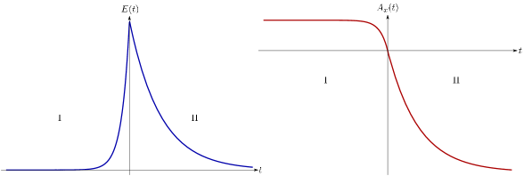
Figure 1: The peak electric field $E\left(t\right)$ and its vector potential $A_{x}\left(t\right)$ (6). Each interval is characterized by a distinct exponential constant which explains the non-symmetrical form of the picture. Here $k_{1}>k_{2}$ has been chosen.

II.2 Dirac equation with peak electric field

To describe the problem in the framework of QED with $t$-electric potential steps it is necessary to solve the Dirac equation for each interval discussed above. In any of them, the Dirac equation in a $d=D+1$ dimensional Minkowski spacetime is, in its Hamiltonian form, represented by

$$i\partial_{t}\psi\left(x\right)=H\left(t\right)\psi\left(x\right)\,,\ \ H\left(t\right)=\gamma^{0}\left(\bm{\gamma}\mathbf{P}+m\right)\,,$$

$$\,P_{x}=-i\partial_{x}-U\left(t\right),\ \ \mathbf{P}_{\bot}=-i\bm{\nabla}_{\perp},\ \ U\left(t\right)=-eA_{x}\left(t\right)\,,$$ (7)

where the index $\perp$ stands for spacial components perpendicular to the electric field, $\mathbf{x}_{\perp}=\left\{x^{2},...,x^{D}\right\}$ and $\mathbf{P}_{\bot}=\left(P^{2},\ldots,P^{D}\right)$. Here $\psi(x)$ is a $2^{[d/2]}$-component spinor ($[d/2]$ stands for the integer part of the ratio $d/2$), $m\neq 0$ is the electron mass, $\gamma^{\mu}$ are the $\gamma$ matrices in $d$ dimensions , $U\left(t\right)$ is the potential energy of one electron, and the relativistic system of units is used throughout in this paper ($\hslash=c=1$).

As customary for $t$-electric steps AdoGavGit15 , solutions of the Dirac equation (7) have the form

$$\psi_{n}\left(x\right)=\exp\left(i\mathbf{pr}\right)\psi_{n}\left(t\right),\;\ n=(\mathbf{p},\sigma)\,,$$

$$\psi_{n}\left(t\right)=\left\{\gamma^{0}i\partial_{t}-\gamma^{1}\left[p_{x}-U\left(t\right)\right]-\bm{\gamma}\mathbf{p}_{\bot}+m\right\}\phi_{n}(t)\,,$$ (8)

where $\psi_{n}\left(t\right)$ and $\phi_{n}(t)$ are spinors which depend on $t$ alone. In fact, these are states with definite momenta $\mathbf{p}$. Substituting Eq. (8) into Dirac equation (7), we obtain a second-order differential equation for the spinor $\phi_{n}(t)$,

$$\left\{\frac{d^{2}}{dt^{2}}+\left[p_{x}-U\left(t\right)\right]^{2}+\pi_{\perp}^{2}-i\gamma^{0}\gamma^{1}\dot{U}\left(t\right)\right\}\phi_{n}\left(t\right)=0\,,\;\pi_{\perp}=\sqrt{\mathbf{p}_{\perp}^{2}+m^{2}}\,.$$ (9)

We separate the spinning variables by the substitution

$$\phi_{n}(t)=\varphi_{n}\left(t\right)v_{\chi,\sigma}\,,$$ (10)

where $v_{\chi,\sigma}$ for $\chi=\pm 1$ and $\sigma=(\sigma_{1},\sigma_{2},\dots,\sigma_{[d/2]-1})$ for $\sigma_{s}=\pm 1$ is a set of constant orthonormalized spinors, satisfying the following equations:

$$\gamma^{0}\gamma^{1}v_{\chi,\sigma}=\chi v_{\chi,\sigma}\,,\ \ v_{\chi,\sigma}^{{\dagger}}v_{\chi^{\prime},\sigma^{\prime}}=\delta_{\chi,\chi^{\prime}}\delta_{\sigma,\sigma^{\prime}\,}.$$ (11)

The quantum numbers $\chi$ and $\sigma_{s}$ describe spin polarization and provide a convenient parametrization of the solutions. Since in ($1+1$) and ($2+1$) dimensions ($d=2,3$) there are no spinning degrees of freedom, the quantum numbers $\sigma$ are absent. In addition, in $d>3$, Eq. (9) allows one to subject the constant spinors $v_{\chi,\sigma}$ to some supplementary conditions that, for example, can be chosen in the form

$$i\gamma^{2s}\gamma^{2s+1}v_{\chi,\sigma}=\sigma_{s}v_{\chi,\sigma}\ \mathrm{for}\ \mathrm{even\ }d\,,$$

$$i\gamma^{2s+1}\gamma^{2s+2}v_{\chi,\sigma}=\sigma_{s}v_{\chi,\sigma}\ \mathrm{for\ odd}\ d\,,$$ (12)

Then the scalar functions $\varphi_{n}\left(t\right)$ have to obey the second-order differential equation

$$\left\{\frac{d^{2}}{dt^{2}}+\left[p_{x}-U\left(t\right)\right]^{2}+\pi_{\perp}^{2}-i\chi\dot{U}\left(t\right)\right\}\varphi_{n}\left(t\right)=0\,.$$ (13)

In $d$ dimensions, for any given set of quantum numbers $\mathbf{p}$, there exist only $J_{(d)}=2^{[d/2]-1}$ different spin states. The projection operator inside the curly brackets in Eq. (8) does not commute with the matrix $\gamma^{0}\gamma^{1}$ and, consequently, transforms $\phi_{n}^{\left(\chi\right)}(x)$ with a given $\chi$ to a linear superposition of functions $\phi_{n}^{\left(+1\right)}(x)$ and $\phi_{n^{\prime}}^{\left(-1\right)}(x)$ with indices $n$ and $n^{\prime}$ corresponding to the same $\mathbf{p}$. For this reason, solutions of (8) differing only by values of $\chi$ and $\sigma_{s}$ are linearly dependent. That is why it is enough to select a particular value of $\chi$ to perform some specific calculations, whose choice shall be explicitly indicated when necessary.

Exact solutions of the Dirac equation with the exponentially decreasing electric field have been obtained by us previously in AdoGavGit14 . Thus, using some results of the latter work, below we summarize the structure of solutions for each interval and unify it in a single presentation. To this aim we introduce new variables $\eta_{j}$,

$$\eta_{1}\left(t\right)=ih_{1}e^{k_{1}t}\,,\ \ \eta_{2}\left(t\right)=ih_{2}e^{-k_{2}t}\,,$$

$$h_{j}=\frac{2eE}{k_{j}^{2}},\ \ j=1,2\,,$$ (14)

in place of $t$ and represent the scalar functions $\varphi_{n}\left(t\right)$ as

$$\varphi_{n}^{j}\left(t\right)=e^{-\eta_{j}/2}\eta_{j}^{\nu_{j}}\tilde{\varphi}^{j}\left(\eta_{j}\right),$$

$$\nu_{j}=\frac{i\omega_{j}}{k_{j}}\,,\ \ \omega_{j}=\sqrt{\pi_{j}^{2}+\pi_{\perp}^{2}}\,,\ \ \pi_{j}=p_{x}-\left(-1\right)^{j}\frac{eE}{k_{j}}\,,$$ (15)

where the subscript $j$ distinguishes quantities associated to the intervals $\mathrm{I}$ ($j=1$) and $\mathrm{II}$ ($j=2$), respectively. Then the functions $\tilde{\varphi}^{j}\left(\eta_{j}\right)$ satisfy the confluent hypergeometric equation BatE53 ,

$$\left[\eta_{j}\frac{d^{2}}{d\eta_{j}^{2}}+\left(c_{j}-\eta_{j}\right)\frac{d}{d\eta_{j}}-a_{j}\right]\tilde{\varphi}^{j}\left(\eta_{j}\right)=0\,,$$

whose parameters are

$$c_{j}=1+2\nu_{j}\,,\ \ a_{j}=\frac{1}{2}\left(1+\chi\right)+\left(-1\right)^{j}\frac{i\pi_{j}}{k_{j}}+\nu_{j}\,.$$ (16)

A fundamental set of solutions for the equation is composed by two linearly independent confluent hypergeometric functions:

$$\Phi\left(a_{j},c_{j};\eta_{j}\right)\ \ \mathrm{and}\ \ \eta_{j}^{1-c_{j}}e^{\eta_{j}}\Phi\left(1-a_{j},2-c_{j};-\eta_{j}\right)\,,$$

where

$$\Phi\left(a,c;\eta\right)=1+\frac{a}{c}\frac{\eta}{1!}+\frac{a\left(a+1\right)}{c\left(c+1\right)}\frac{\eta^{2}}{2!}+\ldots\,.$$ (17)

Thus the general solution of Eq. (13) in the intervals $\mathrm{I}$ and $\mathrm{II}$ can be expressed as the following linear superposition:

$$\varphi_{n}^{j}\left(t\right)=b_{2}^{j}y_{1}^{j}\left(\eta_{j}\right)+b_{1}^{j}y_{2}^{j}\left(\eta_{j}\right)\,,$$

$$y_{1}^{j}\left(\eta_{j}\right)=e^{-\eta_{j}/2}\eta_{j}^{\nu_{j}}\Phi\left(a_{j},c_{j};\eta_{j}\right)\,,$$

$$y_{2}^{j}\left(\eta_{j}\right)=e^{\eta_{j}/2}\eta_{j}^{-\nu_{j}}\Phi\left(1-a_{j},2-c_{j};-\eta_{j}\right)\,,$$ (18)

with constants $b_{1}^{j}$ and $b_{2}^{j}$ being fixed by the initial conditions. The Wronskian of the $y$ functions is

$$y_{1}^{j}\left(\eta_{j}\right)\frac{d}{d\eta_{j}}y_{2}^{j}\left(\eta_{j}\right)-y_{2}^{j}\left(\eta_{j}\right)\frac{d}{d\eta_{j}}y_{1}^{j}\left(\eta_{j}\right)=\frac{1-c_{j}}{\eta_{j}}\,.$$ (19)

It is worth noting that the complete set of solutions for the Klein-Gordon equation,

$$\phi_{n}\left(x\right)=\exp\left(i\mathbf{pr}\right)\varphi_{n}\left(t\right)\,.$$ (20)

can be obtained from the solutions above by setting $\chi=0$ in all formulas. In this case $n=\mathbf{p}$.

With the help of the exact solutions one may write Dirac spinors throughout the time interval $t\in\left(-\infty,+\infty\right)$. As can be seen from (6), the peak electric field is switched on at the infinitely remote past $t\rightarrow-\infty$ and switched off at the infinitely remote future $t\rightarrow+\infty$. At these regions, the exact solutions represent free particles,

$$\ {}_{\zeta}\varphi_{n}\left(t\right)=\ _{\zeta}\mathcal{N}e^{-i\zeta\omega_{1}t}\,\mathrm{\ \ if\ }\ t\rightarrow-\infty,\ \ ^{\zeta}\varphi_{n}\left(t\right)=\ ^{\zeta}\mathcal{N}e^{-i\zeta\omega_{2}t}\mathrm{\ \ if}\ \ t\rightarrow+\infty\,,$$ (21)

respectively, where $\omega_{1}$ denotes energy of initial particles at $t\rightarrow-\infty$, $\omega_{2}$ denotes energy of final particles at $t\rightarrow+\infty$ and $\zeta$ labels electron $\left(\zeta=+\right)$ and positron $\left(\zeta=-\right)$ states. Here$\;{}_{\zeta}\mathcal{N}$ and $\;{}^{\zeta}\mathcal{N}$ are normalization constants with respect to the inner product

$$\left(\psi,\psi^{\prime}\right)=\int\psi^{\dagger}\left(x\right)\psi^{\prime}\left(x\right)d\mathbf{r}\,,\ \ d\mathbf{r}=dx^{1}...dx^{D}\,,$$ (22)

These constants are

$$\ {}_{\zeta}\mathcal{N}=\ _{\zeta}CY\,,\ \ \ ^{\zeta}\mathcal{N}=\ ^{\zeta}CY\,,\ \ Y=V_{\left(d-1\right)}^{-1/2}\,,$$

$${}_{\zeta}C=\left(2\omega_{1}q_{1}^{\zeta}\right)^{-1/2}\,,\ \ \ ^{\zeta}C=\left(2\omega_{2}q_{2}^{\zeta}\right)^{-1/2}\,,$$

$$q_{j}^{\zeta}=\omega_{j}-\chi\zeta\pi_{j}\,,$$ (23)

where $V_{\left(d-1\right)}$ is the spatial volume. By virtue of these properties, electron (positron) states can be selected as follows:

$$\ {}_{+}\varphi_{n}\left(t\right) = \;{}_{+}\mathcal{N}\exp\left(i\pi\nu_{1}/2\right)y_{2}^{1}\left(\eta_{1}\right)\,,\,\ _{-}\varphi_{n}\left(t\right)=\;_{-}\mathcal{N}\exp\left(-i\pi\nu_{1}/2\right)y_{1}^{1}\left(\eta_{1}\right)\,,\ \ t\in\mathrm{I}\,;$$

$$\ {}^{+}\varphi_{n}\left(t\right) = \;{}^{+}\mathcal{N}\exp\left(-i\pi\nu_{2}/2\right)y_{1}^{2}\left(\eta_{2}\right)\,,\,\ ^{-}\varphi_{n}\left(t\right)=\;^{-}\mathcal{N}\exp\left(i\pi\nu_{2}/2\right)y_{2}^{2}\left(\eta_{2}\right)\,,\ \ t\in\mathrm{II}\,.$$ (24)

II.3 $g$ Coefficients and mean numbers of created particles

Taking into account the complete set of exact solutions (18), the functions$\ \ {}_{-}\varphi_{n}\left(t\right)$ and $\ {}^{+}\varphi_{n}\left(t\right)$ can be presented in the form

$$\ \ {}^{+}\varphi_{n}\left(t\right) = \left\{\begin{array}[]{l}g\left({}_{+}|^{+}\right)\ _{+}\varphi_{n}\left(t\right)+\kappa g\left({}_{-}|^{+}\right)\ _{-}\varphi_{n}\left(t\right)\,,\ \ t\in\mathrm{I}\\ \;^{+}\mathcal{N}\exp\left(-i\pi\nu_{2}/2\right)y_{1}^{2}\left(\eta_{2}\right)\,,\ \ \ \ \ \ \ \ \ \ \,t\in\mathrm{II}\end{array}\right.\,,$$ (27)

$$\ {}_{-}\varphi_{n}\left(t\right) = \left\{\begin{array}[]{l}\;_{-}\mathcal{N}\exp\left(-i\pi\nu_{1}/2\right)y_{1}^{1}\left(\eta_{1}\right)\,,\ \ \ \ \ \ \ \ \ \ \ \ \,t\in\mathrm{I}\\ g\left({}^{+}|_{-}\right)\ ^{+}\varphi_{n}\left(t\right)+\kappa g\left({}^{-}|_{-}\right)\ ^{-}\varphi_{n}\left(t\right)\,,\ \ t\in\mathrm{II}\end{array}\right.\,,$$ (30)

for the whole axis $t$, where the coefficients $g$ are the diagonal matrix elements,

$$\left(\ {}_{\zeta^{\prime}}\psi_{l},\ ^{\zeta}\psi_{n}\right)=\delta_{l,n}g\left({}_{\zeta^{\prime}}|^{\zeta}\right),\ \ g\left({}^{\zeta^{\prime}}|_{\zeta}\right)=g\left({}_{\zeta^{\prime}}|^{\zeta}\right)^{\ast}.$$ (31)

These coefficients satisfy the unitary relations

$$\sum_{\varkappa}g\left({}^{\zeta}|_{\varkappa}\right)g\left({}_{\varkappa}|^{\zeta^{\prime}}\right)=\sum_{\varkappa}g\left({}_{\zeta}|^{\varkappa}\right)g\left({}^{\varkappa}|_{\zeta^{\prime}}\right)=\delta_{\zeta,\zeta^{\prime}}\,.$$ (32)

Here the constant $\kappa$ ($\kappa=+1$ above) allows us to cover the Klein-Gordon case, whose details are discussed in Eqs. (37) and (38) below.

The functions$\ {}_{-}\varphi_{n}\left(t\right)$ and $\ {}^{+}\varphi_{n}\left(t\right)$ and their derivatives satisfy the following continuity conditions:

$$\left.\ {}_{-}^{+}\varphi_{n}(t)\right|_{t=-0}=\left.\ {}_{-}^{+}\varphi_{n}(t)\right|_{t=+0}\,,\ \ \left.\partial_{t}\ {}_{-}^{+}\varphi_{n}(t)\right|_{t=-0}=\left.\partial_{t}\ {}_{-}^{+}\varphi_{n}(t)\right|_{t=+0}\,.$$ (33)

Using Eq. (33) and the Wronskian (19), one can find each coefficient $g\left({}_{\zeta}|^{\zeta^{\prime}}\right)$ and $g\left({}^{\zeta}|_{\zeta^{\prime}}\right)$ in Eqs. (27) and (30). For example, applying these conditions to the set (27), the coefficient $g\left({}_{-}|^{+}\right)$ takes the form

$$g\left({}_{-}|^{+}\right)=\mathcal{C}\Delta\,,\ \ \mathcal{C}=-\frac{1}{2}\sqrt{\frac{q_{1}^{-}}{\omega_{1}q_{2}^{+}\omega_{2}}}\exp\left[\frac{i\pi}{2}\left(\nu_{1}-\nu_{2}\right)\right]\,,$$

$$\Delta=\left.\left[k_{1}h_{1}y_{1}^{2}\left(\eta_{2}\right)\frac{d}{d\eta_{1}}y_{2}^{1}\left(\eta_{1}\right)+k_{2}h_{2}y_{2}^{1}\left(\eta_{1}\right)\frac{d}{d\eta_{2}}y_{1}^{2}\left(\eta_{2}\right)\right]\right|_{t=0}\,.$$ (34)

Alternatively, we obtain from the set (27)

$$g\left({}^{+}|_{-}\right)=\mathcal{C}^{\prime}\Delta^{\prime}\,,\ \ \mathcal{C}^{\prime}=-\frac{1}{2}\sqrt{\frac{q_{2}^{+}}{\omega_{1}q_{1}^{-}\omega_{2}}}\exp\left[\frac{i\pi}{2}\left(\nu_{2}-\nu_{1}\right)\right]\,,$$

$$\Delta^{\prime}=\left\{k_{2}h_{2}y_{1}^{1}\left(\eta_{1}\right)\frac{d}{d\eta_{2}}y_{2}^{2}\left(\eta_{2}\right)+k_{1}h_{1}y_{2}^{2}\left(\eta_{2}\right)\frac{d}{d\eta_{1}}y_{1}^{1}\left(\eta_{1}\right)\right\}_{t=0}\,.$$ (35)

Comparing Eqs. (34) and (35) one can easily verify that the symmetry under a simultaneous change $k_{1}\leftrightarrows k_{2}$ and $\pi_{1}\leftrightarrows-\pi_{2}$ holds,

$$g\left({}^{+}|_{-}\right)\leftrightarrows g\left({}_{-}|^{+}\right)\,.$$ (36)

A formal transition to the Klein-Gordon case can be performed by setting $\chi=0$ and $\kappa=-1$ in Eqs. (27) and (30), and by replacing the normalization factors ${}_{\zeta}C,\ ^{\zeta}C$ written in (23) by

$$\ {}_{\zeta}C=\left(2\omega_{1}\right)^{-1/2}\,,\ \ \ ^{\zeta}C=\left(2\omega_{2}\right)^{-1/2}\,.$$ (37)

After these substitutions, the coefficient $g\left({}_{-}|^{+}\right)$ for scalar particles reads

$$g\left({}_{-}|^{+}\right)=\mathcal{C}_{\mathrm{sc}}\left.\Delta\right|_{\chi=0}\,,\ \ \mathcal{C}_{\mathrm{sc}}=\left(4\omega_{1}\omega_{2}\right)^{-1/2}\exp\left[i\pi\left(\nu_{1}-\nu_{2}\right)/2\right]\,,$$ (38)

with $\Delta$ given by Eq. (34). In this case it is worth noting that the symmetry under the simultaneous change $k_{1}\leftrightarrows k_{2}$ and $\pi_{1}\leftrightarrows-\pi_{2}$ holds as

$$g\left({}^{+}|_{-}\right)\leftrightarrows-g\left({}_{-}|^{+}\right)\,.$$ (39)

Note that for scalar particles the coefficients $g$ satisfy the unitary relations

$$\sum_{\varkappa}\varkappa g\left({}^{\zeta}|_{\varkappa}\right)g\left({}_{\varkappa}|^{\zeta^{\prime}}\right)=\sum_{\varkappa}\varkappa g\left({}_{\zeta}|^{\varkappa}\right)g\left({}^{\varkappa}|_{\zeta^{\prime}}\right)=\zeta\delta_{\zeta,\zeta^{\prime}}\,.$$ (40)

Using a unitary transformation $V$ between the initial and final Fock spaces, see FGS , one finds that the differential mean number of electron-positron pairs created from the vacuum can be expressed via the coefficients $g$ as

$$N_{n}^{\mathrm{cr}}=\left|g\left({}_{-}|^{+}\right)\right|^{2}$$ (41)

both for fermions and bosons. Then the total number of  created pairs is given by the sum

$$N=\sum_{n}N_{n}^{\mathrm{cr}}=\sum_{n}\left|g\left({}_{-}\left|{}^{+}\right.\right)\right|^{2}$$ (42)

and the vacuum-to-vacuum transition probability reads

$$P_{v}=\exp\left\{\kappa\sum_{n}\ln\left[1-\kappa N_{n}^{\mathrm{cr}}\right]\right\}\,.$$ (43)

For Dirac particles, using $g\left({}_{-}|^{+}\right)$ given by Eq. (34), we find in the case under consideration

$$N_{n}^{\mathrm{cr}}=\left|\mathcal{C}\Delta\right|^{2}\,.$$ (44)

For scalar particles, using $g\left({}_{-}|^{+}\right)$ given by Eq. (38) the same quantity has the form

$$N_{n}^{\mathrm{cr}}=\left|\mathcal{C}_{\mathrm{sc}}\left.\Delta\right|_{\chi=0}\right|^{2}\,.$$ (45)

It is clear that $N_{n}^{\mathrm{cr}}$ is a function of modulus squared of transversal momentum, $\mathbf{p}_{\perp}^{2}$. It follows from Eq. (36) and (39), respectively, that $N_{n}^{\mathrm{cr}}$ is invariant under the simultaneous change $k_{1}\leftrightarrows k_{2}$ and $\pi_{1}\leftrightarrows-\pi_{2}$ for both fermions and bosons. Then if $k_{1}=k_{2}$, $N_{n}^{\mathrm{cr}}$ appears to be an even function of longitudinal momentum $p_{x}$ too.

III Slowly varying field

III.1 Differential quantities

We are primarily interested in a strong field, when $N_{n}^{\mathrm{cr}}$ are not necessarily small in some ranges of quantum numbers and semiclassical calculations cannot be applied. The inverse parameters $k_{1}^{-1}$, $k_{2}^{-1}$ represent scales of time duration for increasing and decreasing phases of the electric field. In particular, we have a slowly varying field at small values of both $k_{1},k_{2}\rightarrow 0$. This case can be considered as a new two-parameter regularization for a constant electric field [additional to the known one-parameter regularizations by the Sauter-like electric field, $E\cosh^{-2}\left(t/T_{\mathrm{S}}\right)$, and the $T$-constant electric field (an electric field which effectively acts during a sufficiently large but finite time interval $T$)]. Let us consider only this case, supposing that $k_{1}$ and $k_{2}$ are sufficiently small, obeying the conditions

$$\min\left(h_{1},h_{2}\right)\gg\max\left(1,m^{2}/eE\right)\,.$$ (46)

Let us analyze how the numbers $N_{n}^{\mathrm{cr}}$ depend on the parameters $p_{x}$ and $\pi_{\perp}$. It can be seen from semiclassical analysis that $N_{n}^{\mathrm{cr}}$ is exponentially small in the range of very large $\pi_{\perp}\gtrsim\min\left(eEk_{1}^{-1},eEk_{2}^{-1}\right)$. Then the range of fixed $\pi_{\perp}$ is of interest, and in what follows, we assume that

$$\sqrt{\lambda}<K_{\bot}\,,\ \ \lambda=\frac{\pi_{\perp}^{2}}{eE}\,,$$ (47)

where $K_{\bot}$ is any given number satisfying the condition

$$\min\left(h_{1},h_{2}\right)\gg K_{\bot}^{2}\gg\max\left(1,m^{2}/eE\right)\,.$$ (48)

By virtue of symmetry properties of $N_{n}^{\mathrm{cr}}$ discussed above, one can only consider $p_{x}$ either positive or negative. Let us, for example, consider the interval $-\infty<p_{x}\leq 0$. In this case $\pi_{2}$ is negative and large, $-\pi_{2}\geq eE/k_{2}$, while $\pi_{1}$ varies from positive to negative values, $-\infty<\pi_{1}\leq eE/k_{1}$. The case of large negative $\pi_{1}$, $-2\pi_{1}/k_{1}>K_{1}$, where $K_{1}$ is any given large number, $K_{1}\gg K_{\bot}$, is quite simple. In this case, using the appropriate asymptotic expressions of the confluent hypergeometric function one can see that $N_{n}^{\mathrm{cr}}$ is negligibly small. To see this, Eq. (108) in Appendix A is useful in the range $h_{1}\gtrsim-2\pi_{1}/k_{1}>K_{1}$ and the expression for large $c_{2}$ with fixed $a_{2}$ and $h_{2}$ and the expression for large $c_{1}$ with fixed $a_{1}-c_{1}$ and $h_{1}$, given in BatE53 , are useful in the range $-2\pi_{1}/k_{1}\gg h_{1}$.

We expect a significant contribution in the range

$$h_{1}\geq 2\pi_{1}/k_{1}>-K_{1},$$ (49)

that can be divided in four subranges

$$\mathrm{(a)} \;h_{1}\geq 2\pi_{1}/k_{1}>h_{1}\left[1-\left(\sqrt{h_{1}}g_{2}\right)^{-1}\right],$$

$$\mathrm{(b)} \;h_{1}\left[1-\left(\sqrt{h_{1}}g_{2}\right)^{-1}\right]>2\pi_{1}/k_{1}>h_{1}\left(1-\varepsilon\right),$$

$$\mathrm{(c)} \;h_{1}\left(1-\varepsilon\right)>2\pi_{1}/k_{1}>h_{1}/g_{1},$$

$$\mathrm{(d)} \;h_{1}/g_{1}>2\pi_{1}/k_{1}>-K_{1},$$ (50)

where $g_{1}$, $g_{2}$, and $\varepsilon$ are any given numbers satisfying the condition $g_{1}$ $\gg 1$, $g_{2}$ $\gg 1$, and $\varepsilon\ll 1$. .Note that $\tau_{1}=-ih_{1}/\left(2-c_{1}\right)\approx\frac{h_{1}k_{1}}{2\left|\pi_{1}\right|}$ in the subranges (a), (b), and (c) and $\tau_{2}=ih_{2}/c_{2}\approx\frac{h_{2}k_{2}}{2\left|\pi_{2}\right|}$ in the whole range (49). In these subranges we have for $\left|\tau_{2}\right|$

$$\mathrm{(a)} \;1\leq\tau_{2}^{-1}<\left[1+\left(\sqrt{h_{2}}g_{2}\right)^{-1}\right],$$

$$\mathrm{(b)} \;\left[1+\left(\sqrt{h_{2}}g_{2}\right)^{-1}\right]<\tau_{2}^{-1}<\left(1+\varepsilon k_{2}/k_{1}\right),$$

$$\mathrm{(c)} \;\left(1+\varepsilon k_{2}/k_{1}\right)<\tau_{2}^{-1}<\left[1+k_{2}/k_{1}\left(1-1/g_{1}\right)\right],$$

$$\mathrm{(d)} \;\left[1+k_{2}/k_{1}\left(1-1/g_{1}\right)\right]<\tau_{2}^{-1}\lesssim\left(1+k_{2}/k_{1}\right).$$ (51)

We see that $\tau_{1}-1\rightarrow 0$ and $\tau_{2}-1\rightarrow 0$ in the range (a), while $\left|\tau_{1}-1\right|\sim 1$ in the range (c), and $\left|\tau_{2}-1\right|\sim 1$ in the ranges (c) and (d). In the range (b) these quantities vary from their values in the ranges (a) and (c).

In the range (a) we can use the asymptotic expression of the confluent hypergeometric function given by Eq. (98) in Appendix A. Using Eqs. (104), (105), and (106) obtained in Appendix A, we finally find the leading term as

$$N_{n}^{\mathrm{cr}}=e^{-\pi\lambda}\left[1+O\left(\left|\mathcal{Z}_{1}\right|\right)\right],$$ (52)

for fermions and bosons, where $\max\left|\mathcal{Z}_{1}\right|\lesssim g_{2}^{-1}$ . In the range (c), we use the asymptotic expression of the confluent hypergeometric function given by Eq. (108) in Appendix A. Then we find that

$$N_{n}^{\mathrm{cr}}=e^{-\pi\lambda}\left[1+O\left(\left|\mathcal{Z}_{1}\right|\right)^{-1}+O\left(\left|\mathcal{Z}_{2}\right|\right)^{-1}\right],$$ (53)

where $\max\left|\mathcal{Z}_{1}\right|^{-1}\lesssim\sqrt{g_{1}/h_{1}}$ and $\max\left|\mathcal{Z}_{2}\right|^{-1}\lesssim g_{2}^{-1}$. Using the asymptotic expression Eq. (98) and taking into account Eq. (52) and (53), we can estimate that $N_{n}^{\mathrm{cr}}\sim e^{-\pi\lambda}$ in the range (b). In the range (d), the confluent hypergeometric function $\Phi\left(a_{2},c_{2};ih_{2}\right)$ is approximated by Eq. (107) and the function $\Phi\left(1-a_{1},2-c_{1};-ih_{1}\right)$ is approximated by Eq. (109) given in Appendix A. In this range the differential mean numbers in the leading-order approximation are

$$N_{n}^{\mathrm{cr}}\approx\frac{\exp\left[-\frac{\pi}{k_{1}}\left(\omega_{1}-\pi_{1}\right)\right]}{\sinh\left(2\pi\omega_{1}/k_{1}\right)}\times\left\{\begin{array}[]{l}\sinh\left[\pi\left(\omega_{1}+\pi_{1}\right)/k_{1}\right]\ \mathrm{for\ fermions}\\ \cosh\left[\pi\left(\omega_{1}+\pi_{1}\right)/k_{1}\right]\ \mathrm{for\ bosons}\end{array}\right.\,.$$ (54)

It is clear that $N_{n}^{\mathrm{cr}}$ given by Eqs. (54) tends to Eq. (53), $N_{n}^{\mathrm{cr}}\rightarrow e^{-\pi\lambda}$, when $\pi_{1}\gg\pi_{\bot}$. Consequently, the forms (54) are valid in the whole range (49). Assuming $m/k_{1}\gg 1$, we see that  values of $N_{n}^{\mathrm{cr}}$ given by Eqs. (54) are negligible in the range $\pi_{1}\lesssim\pi_{\bot}$. Then we find for bosons and fermions that significant value of $N_{n}^{\mathrm{cr}}$ is in the range $\pi_{\bot}<\pi_{1}\leqslant eE/k_{1}$ and it has the form

$$N_{n}^{\mathrm{cr}}\approx\exp\left[-\frac{2\pi}{k_{1}}\left(\omega_{1}-\pi_{1}\right)\right].$$ (55)

Considering positive $p_{x}>0$, we can take into account that exact $N_{n}^{\mathrm{cr}}$ is invariant under the simultaneous exchange $k_{1}\leftrightarrows k_{2}$ and $\pi_{1}\leftrightarrows-\pi_{2}$. In this case $\pi_{1}$ is positive and large, $\pi_{1}>eE/k_{1}$, while $\pi_{2}$ varies from negative to positive values, $-eE/k_{2}<\pi_{2}<\infty$. We find a significant contribution in the range

$$-h_{2}<2\pi_{2}/k_{2}<K_{2},$$ (56)

where $K_{2}$ is any given large number, $K_{2}\gg K_{\bot}$. In this range, similarly to the case of the negative $p_{x}$, the differential mean numbers in the leading-order approximation are

$$N_{n}^{\mathrm{cr}}\approx\frac{\exp\left[-\frac{\pi}{k_{2}}\left(\omega_{2}+\pi_{2}\right)\right]}{\sinh\left(2\pi\omega_{2}/k_{2}\right)}\times\left\{\begin{array}[]{c}\sinh\left[\pi\left(\omega_{2}-\pi_{2}\right)/k_{2}\right]\ \mathrm{for\ fermions}\\ \cosh\left(\pi\left(\omega_{2}-\pi_{2}\right)/k_{2}\right)\ \mathrm{for\ bosons}\end{array}\right.\,.$$ (57)

Assuming $m/k_{2}\gg 1$, we find for bosons and fermions that significant value of $N_{n}^{\mathrm{cr}}$ is in the range $-eE/k_{2}<\pi_{2}<-\pi_{\bot}$ and it has a form

$$N_{n}^{\mathrm{cr}}\approx\exp\left[-\frac{2\pi}{k_{2}}\left(\omega_{2}+\pi_{2}\right)\right].$$ (58)

Consequently, the quantity $N_{n}^{\mathrm{cr}}$ is almost constant over the wide range of longitudinal momentum $p_{x}$ for any given $\lambda$ satisfying Eq. (47). When $h_{1},h_{2}\rightarrow\infty$, one obtains the well-known result in a constant uniform electric field Nikis70a ; Nikis70b ,

$$N_{n}^{\mathrm{cr}}\rightarrow N_{n}^{\mathrm{uni}}=e^{-\pi\lambda}.$$ (59)

III.2 Total quantities

In this subsection we estimate the total number $N^{\mathrm{cr}}$ of pairs created by the peak electric field. To compute this number, one has to sum the corresponding differential mean numbers $N_{n}^{\mathrm{cr}}$ over the momenta $\mathbf{p}$ and, in the Fermi case, to  sum over the spin projections. Once $N_{n}^{\mathrm{cr}}$ does not depend on the spin variables, the latter sum results in a multiplicative numerical factor $J_{(d)}=2^{\left[d/2\right]-1}$ for fermions ($J_{\left(d\right)}=1$ for bosons). Then replacing the sum over the momenta in Eq. (42) by an integral, the total number of pairs created from the vacuum takes the form

$$N^{\mathrm{cr}}=\frac{V_{\left(d-1\right)}}{(2\pi)^{d-1}}J_{(d)}\int d\mathbf{p}N_{n}^{\mathrm{cr}}\,.$$ (60)

Due to the structure of the coefficients $g\left({}_{-}|^{+}\right)$ presented in section II.3, it is clear that a direct integration of combinations of hypergeometric functions involved in the absolute value of (34) and (38) is overcomplicated. Nevertheless the analysis presented in section III.1 reveals that the dominant contributions for particle creation by a slowly varying field occurs in the ranges of large kinetic momenta, whose differential quantities have the asymptotic forms (55) for $p_{x}<0$ and (58) for $p_{x}>0$. Therefore, one may represent the total number (60) as

$$N^{\mathrm{cr}}=V_{\left(d-1\right)}n^{\mathrm{cr}}\,,\ \ n^{\mathrm{cr}}=\frac{J_{(d)}}{(2\pi)^{d-1}}\int_{\sqrt{\lambda}<K_{\bot}}d\mathbf{p}_{\bot}I_{\mathbf{p}_{\bot}},\ \ I_{\mathbf{p}_{\bot}}=I_{\mathbf{p}_{\bot}}^{\left(1\right)}+I_{\mathbf{p}_{\bot}}^{\left(2\right)},$$

$$I_{\mathbf{p}_{\bot}}^{\left(1\right)}=\int_{-\infty}^{0}dp_{x}N_{n}^{\mathrm{cr}}\approx\int_{\pi_{\perp}}^{eE/k_{1}}d\pi_{1}\exp\left[-\frac{2\pi}{k_{1}}\left(\omega_{1}-\pi_{1}\right)\right]\,,$$

$$I_{\mathbf{p}_{\bot}}^{\left(2\right)}=\int_{0}^{\infty}dp_{x}N_{n}^{\mathrm{cr}}\approx\int_{\pi_{\perp}}^{eE/k_{2}}d\left|\pi_{2}\right|\exp\left[-\frac{2\pi}{k_{2}}\left(\omega_{2}-\left|\pi_{2}\right|\right)\right]\,.$$ (61)

Using the change of the variables

$$s=\frac{2}{k_{1}\lambda}\left(\omega_{1}-\pi_{1}\right)\,,$$

and neglecting exponentially small contributions, we represent the quantity $I_{\mathbf{p}_{\bot}}^{\left(1\right)}$ as

$$I_{\mathbf{p}_{\bot}}^{\left(1\right)}\approx\int_{1}^{\infty}\frac{ds}{s}\omega_{1}e^{-\pi\lambda s}\,.$$ (62)

Similarly, using the change of variables

$$s=\frac{2}{k_{2}\lambda}\left(\omega_{2}-\left|\pi_{2}\right|\right)\,,$$

we represent the quantity $I_{\mathbf{p}_{\bot}}^{\left(2\right)}$ as

$$I_{\mathbf{p}_{\bot}}^{\left(2\right)}\approx\int_{1}^{\infty}\frac{ds}{s}\omega_{2}e^{-\pi\lambda s}\,.$$ (63)

The leading contributions for both integrals (62) and (63) come from the range near $s\rightarrow 1$, where $\omega_{1}$ and $\omega_{2}$ are approximately given by,

$$\omega_{1}\approx\frac{eE}{sk_{1}}\,,\ \ \omega_{2}\approx\frac{eE}{sk_{2}}\,.$$

Consequently the leading term in $I_{\mathbf{p}_{\bot}}$ (61) takes the following final form,

$$I_{\mathbf{p}_{\bot}}\approx\left(\frac{eE}{k_{1}}+\frac{eE}{k_{2}}\right)\int_{1}^{\infty}\frac{ds}{s^{2}}e^{-\pi\lambda s}=eE\left(\frac{1}{k_{1}}+\frac{1}{k_{2}}\right)e^{-\pi\lambda}G\left(1,\pi\lambda\right),$$ (64)

where

$$G\left(\alpha,x\right)=\int_{1}^{\infty}\frac{ds}{s^{\alpha+1}}e^{-x\left(s-1\right)}=e^{x}x^{\alpha}\Gamma\left(-\alpha,x\right),$$ (65)

and $\Gamma\left(-\alpha,x\right)$ is the incomplete gamma function.

Neglecting the exponentially small contribution, one can represent the integral over $\mathbf{p}_{\bot}$ in Eq. (61) (where $I_{\mathbf{p}_{\bot}}$ is given by Eq. (64)) as

$$\int_{\sqrt{\lambda}<K_{\bot}}d\mathbf{p}_{\bot}I_{\mathbf{p}_{\bot}}\approx\int_{\sqrt{\lambda}<\infty}d\mathbf{p}_{\bot}I_{\mathbf{p}_{\bot}}.$$

Then calculating the Gaussian integral,

$$\int d\mathbf{p}_{\bot}\exp\left(-\pi s\frac{\mathbf{p}_{\bot}^{2}}{eE}\right)=\left(\frac{eE}{s}\right)^{d/2-1},$$ (66)

we find

$$n^{\mathrm{cr}}=r^{\mathrm{cr}}\left(\frac{1}{k_{1}}+\frac{1}{k_{2}}\right)G\left(\frac{d}{2},\pi\frac{m^{2}}{eE}\right),\;\;r^{\mathrm{cr}}=\frac{J_{(d)}\left(eE\right)^{d/2}}{(2\pi)^{d-1}}\exp\left\{-\pi\frac{m^{2}}{eE}\right\}.$$ (67)

Using the considerations presented above, one can perform the summation (integration) in Eq. (43) to obtain the vacuum-to-vacuum probability $P_{v}$,

$$P_{v}=\exp\left(-\mu N^{\mathrm{cr}}\right),\;\;\mu=\sum_{l=0}^{\infty}\frac{(-1)^{(1-\kappa)l/2}\epsilon_{l+1}}{(l+1)^{d/2}}\exp\left(-l\pi\frac{m^{2}}{eE}\right)\;,$$

$$\epsilon_{l}=G\left(\frac{d}{2},l\pi\frac{m^{2}}{eE}\right)\left[G\left(\frac{d}{2},\pi\frac{m^{2}}{eE}\right)\right]^{-1}.$$ (68)

These results allow us to establish an immediate comparison with the one-parameter regularizations of the constant field, namely the $T$-constant and Sauter-like electric fields GavGit96 . We note that in all these cases the quantity is quasiconstant over the wide range of the longitudinal momentum $p_{x}$ for any given $\lambda,$ i.e., $N_{n}^{\mathrm{cr}}\sim e^{-\pi\lambda}$. Pair creation effects in such fields are proportional to increments of longitudinal kinetic momentum, $\Delta U=e\left|A_{x}\left(+\infty\right)-A_{x}\left(-\infty\right)\right|$, which are

$$\Delta U_{\mathrm{p}} = eE\left(k_{1}^{-1}+k_{2}^{-1}\right)\;\mathrm{for\;peak\ field,}$$

$$\Delta U_{\mathrm{T}} = eET\;\;\mathrm{for\;T}\text{{-}}\mathrm{const\ field,}$$

$$\Delta U_{\mathrm{S}} = 2eET_{\mathrm{S}}\;\;\mathrm{for\;Sauter}\text{{-}}\mathrm{like\ field}\text{.}$$ (69)

This fact allows one to compare pair creation effects in such fields. Using the quantities introduced, we can represent the densities $n^{\mathrm{cr}}$ as follows:

$$n^{\mathrm{cr}} = r^{\mathrm{cr}}\frac{\Delta U_{\mathrm{p}}}{eE}G\left(\frac{d}{2},\pi\frac{m^{2}}{eE}\right),\ \mathrm{for\;peak\ field,}$$

$$n^{\mathrm{cr}} = r^{\mathrm{cr}}\frac{\Delta U_{\mathrm{T}}}{eE}\;\;\mathrm{for\;T}\text{{-}}\mathrm{constant\ field},$$

$$n^{\mathrm{cr}} = r^{\mathrm{cr}}\frac{\Delta U_{\mathrm{S}}}{2eE}\delta\;\mathrm{for\;Sauter}\text{{-}}\mathrm{like\ field},$$ (70)

where

$$\delta=\int_{0}^{\infty}dtt^{-1/2}(t+1)^{-\left(d-2\right)/2}\exp\left(-t\pi\frac{m^{2}}{eE}\right)=\sqrt{\pi}\Psi\left(\frac{1}{2},-\frac{d-2}{2};\pi\frac{m^{2}}{eE}\right),$$

and $\Psi\left(a,b;x\right)$ is the confluent hypergeometric function BatE53 .

Thus, for a given magnitude of the electric field $E$ one can compare the pair creation effects in fields with equal increment of the longitudinal kinetic momentum, or one can determine such increments of the longitudinal kinetic momenta, for which particle creation effects are the same. In Eq.(69) $T$ is the time duration of the $T$-constant field. Equating the densities $n^{\mathrm{cr}}$ for Sauter-like field and for the peak field to the density $n^{\mathrm{cr}}$ for the $T$-constant field, we find an effective duration time $T_{eff}$ in both cases,

$$T_{eff} = T_{\mathrm{S}}\delta\;\mathrm{for\;Sauter}\text{{-}}\mathrm{like\ field},$$

$$T_{eff} = \left(k_{1}^{-1}+k_{2}^{-1}\right)G\left(\frac{d}{2},\pi\frac{m^{2}}{eE}\right)\;\mathrm{for\;the\ peak\ field}.$$ (71)

By the definition $T_{eff}=T$ for the $T$-constant field. One can say that the Sauter-like and the peak electric fields with the same $T_{eff}=T$ are equivalent to the $T$-constant field in pair production.

If the electric field $E$ is weak, $m^{2}/eE\gg$ $1$, one can use asymptotic expressions for the $\Psi$-function and the incomplete gamma function. Thus, we obtain

$$G\left(\frac{d}{2},\pi\frac{m^{2}}{eE}\right)\approx\frac{eE}{\pi m^{2}},\ \ \delta\approx\sqrt{eE}/m\ .$$ (72)

If the electric field $E$ is strong enough, $m^{2}/eE\ll 1$, it follows from a corresponding representation for the $\Psi$-function, see Ref. BatE53 , that its leading term does not depend on the dimensionless parameter $m^{2}/eE$ and reads

$$\Psi\left(\frac{1}{2},-\frac{d-2}{2};\pi\frac{m^{2}}{eE}\right)\approx\Gamma\left(d/2\right)/\Gamma\left(d/2+1/2\right).$$ (73)

Then, for example, $\delta\approx\pi/2$ if $d=3$ and $\delta\approx 4/3$ if $d=4$. The leading term of $G$-function, which is given by Eq. (65), does not depend on the parameter $m^{2}/eE$ either,

$$G\left(\frac{d}{2},\pi\frac{m^{2}}{eE}\right)\approx\frac{2}{d}.$$ (74)

It is clear that there is a time range where Sauter-like and the peak electric fields coincide with a $T$-constant field. Out of this range both these fields have an exponential behavior and can be compared. Assuming $k_{1}\sim k_{2}$, we have

$$\dot{U} \approx eEe^{-2\left|t\right|/T_{\mathrm{S}}}\;\mathrm{if}\;\left|t\right|/T_{\mathrm{S}}\gg 1\;\mathrm{for\;Sauter}\text{{-}}\mathrm{like\ field},$$

$$\dot{U} \approx eEe^{-k_{1}\left|t\right|}\;\mathrm{if}\;k_{1}\left|t\right|\gg 1\;\mathrm{for\;peak\ field}.$$ (75)

If the field is weak, $m^{2}/eE\gg$ $1$, we see that

$$k_{1}T_{\mathrm{S}}=\frac{2\sqrt{eE}}{\pi m}\ll 1,$$

that is, the peak electric field switches on and off much more slowly than the Sauter-like field. If the field is strong, $m^{2}/eE\ll 1$, this dimensionless parameter turns to unity,

$$k_{1}T_{\mathrm{S}}=\left\{\begin{array}[]{l}8/\left(3\pi\right)\;\;\mathrm{if}\;d=3\\ 3/4\;\;\mathrm{if}\;d=4\end{array}\right..$$

In this case, the peak electric field switches on and off not much slowly than the Sauter-like field.

Another global quantity is the vacuum-to-vacuum transition probability $P_{v}$. It is given by Eq. (68) for the peak field and has the form similar to that for the $T$-constant and the Sauter-like fields with the corresponding $N^{\mathrm{cr}}$, and

$$\epsilon_{l} = \epsilon_{l}^{\mathrm{T}}=1\;\mathrm{for\;T}\text{{-}}\mathrm{constant\ field},$$

$$\epsilon_{l} = \epsilon_{l}^{\mathrm{S}}=\delta^{-1}\sqrt{\pi}\Psi\left(\frac{1}{2},-\frac{d-2}{2};l\pi\frac{m^{2}}{eE}\right)\;\mathrm{for\;Sauter}\text{{-}}\mathrm{like\ field}.$$ (76)

If the field is weak, $m^{2}/eE\gg 1$, then $\;\epsilon_{l}^{\mathrm{S}}\approx l^{-1/2}$ for the Sauter-like field and $\epsilon_{l}\approx l^{-1}$ for the peak field. Then $\mu\approx 1$ for both fields and we see that the identification with $T_{eff}=T$, given by Eq. (71), is the same as the one extracted from the comparison of total densities $n^{\mathrm{cr}}$. In the case of a strong field, $m^{2}/eE\ll 1$, all the terms with different $\epsilon_{l}^{\mathrm{S}}$ and $\epsilon_{l}$ contribute significantly to the sum in Eq. (68) if $l\pi m^{2}/eE\sim 1$, and the $\mu$ quantities differ essentially from the case of the $T$-constant field. However, for a very strong field, $l\pi m^{2}/eE\ll 1$, the leading contribution for $\epsilon_{l}$ has a quite simple form $\epsilon_{l}^{\mathrm{S}}\approx\epsilon_{l}\approx 1$. In this case the quantities $\mu$ are the same for all these fields, namely

$$\mu\approx\sum_{l=0}^{\infty}\frac{(-1)^{(1-\kappa)l/2}}{(l+1)^{d/2}},$$

and the identification with $T_{eff}=T$ is the same as the one extracted from the comparison of the total densities $n^{\mathrm{cr}}$.

It is clear that different total quantities, such as the total number of created pairs and the vacuum-to-vacuum transition probability  discussed above, in the general case lead to different identifications with $T_{eff}=T$. We believe that some of these quantities are more adequate for such an identification. In this connection, it should be noted that in small-gradient fields, the total vacuum mean values, such as mean electric currents and the mean energy-momentum tensor, are usually of interest; see, e.g. Refs. GavGit08 ; GavGit08b ; GavGitY12 . These total quantities are represented by corresponding sums of differential numbers of created particles. Therefore, relations between the total numbers and parameters $\Delta U_{\mathrm{p}}$, $\Delta U_{\mathrm{T}}$, and $\Delta U_{\mathrm{S}}$ derived above are also important. Such relations derived from the vacuum-to-vacuum transition probability $P_{v}$ are interesting in semiclassical approaches based on Schwinger’s technics Sch51 . We recall that the semiclassical approaches work in the case of weak external fields $m^{2}/eE\gg$ $1$. It should be noted that in the case of a strong field when the semiclassical approach is not applicable, the probability $P_{v}$ has no direct relation to vacuum mean values of the above discussed physical quantities.

IV Configurations with sharp fields

IV.1 Short pulse field

Choosing certain parameters of the peak field, one can obtain electric fields that exist only for a short time in a vicinity of the time instant $t=0$. The latter fields switch on and/or switch off “abruptly” near the time instant $t=0$. Let us consider large parameters $k_{1}$, $k_{2}\rightarrow\infty$ with a fixed ratio $k_{1}/k_{2}$. The corresponding asymptotic potentials, $U\left(+\infty\right)=eEk_{2}^{-1}$ and $U\left(-\infty\right)=-eEk_{1}^{-1}$ define finite increments of the longitudinal kinetic momenta $\Delta U_{1}$ and $\Delta U_{2}$ for increasing and decreasing parts, respectively,      ,

$$\Delta U_{1}=U\left(0\right)-U\left(-\infty\right)=eEk_{1}^{-1},\;\;\Delta U_{2}=U\left(+\infty\right)-U\left(0\right)=eEk_{2}^{-1}.$$ (77)

Such a case corresponds to a very short pulse of the electric field. At the same time this configuration imitates well enough a $t$-electric rectangular potential step (it is an analog of the Klein step, which is an $x$-electric rectangular step; see Ref. GavGit15 ) and coincides with it as $k_{1}$, $k_{2}\rightarrow\infty$. Thus, these field configurations can be considered as regularizations of rectangular step. We assume that sufficiently large $k_{1}$ and $k_{2}$ satisfy the following inequalities:

$$\Delta U_{1}/k_{1}\ll 1,\;\;\Delta U_{2}/k_{2}\ll 1,\;\;\max\left(\omega_{1}/k_{1},\omega_{2}/k_{2}\right)\ll 1$$ (78)

for any given $\pi_{\perp}$ and $\pi_{1,2}=p_{x}-U\left(\mp\infty\right)$. In this case the confluent hypergeometric function can be approximated by the first two terms in Eq. (17), which are $\Phi\left(a,c;\eta\right)$, $c_{j}\approx 1$, and $\ \ a_{j}\approx\left(1+\chi\right)/2$. Then for fermions, we obtain the result

$$N_{n}^{\mathrm{cr}}=\frac{\left(\omega_{1}+\pi_{1}\right)\left(\Delta U_{2}+\Delta U_{1}+\omega_{2}-\omega_{1}\right)^{2}}{4\omega_{1}\omega_{2}\left(\omega_{2}-\pi_{2}\right)}$$ (79)

which does not depend on $k_{1,2}$. For bosons, we obtain

$$N_{n}^{\mathrm{cr}}=\frac{\left(\omega_{2}-\omega_{1}\right)^{2}}{4\omega_{1}\omega_{2}}.$$ (80)

In contrast to the Fermi case, where $N_{n}^{\mathrm{cr}}\leq 1$, in the Bose case, the differential numbers $N_{n}^{\mathrm{cr}}$ are unbounded in two ranges of the longitudinal kinetic momenta, in the range where $\omega_{1}/\omega_{2}\rightarrow\infty$ and in the range where $\omega_{2}/\omega_{1}\rightarrow\infty$. In these ranges they are

$$N_{n}^{\mathrm{cr}}\approx\frac{1}{4}\max\left\{\omega_{1}/\omega_{2},\omega_{2}/\omega_{1}\right\}.$$ (81)

If $k_{1}=k_{2}$ (in this case $\Delta U_{2}=\Delta U_{1}=\Delta U/2$), we can compare the above results with the results of the regularization of rectangular steps by the Sauter-like potential AdoGavGit15 , obtained for a small $T_{\mathrm{S}}\rightarrow 0$ and constant $\Delta U=2eET_{\mathrm{S}}$ under the conditions $\Delta UT_{\mathrm{S}}\ll 1$ and $\max\left\{T_{\mathrm{S}}\omega_{1},T_{\mathrm{S}}\omega_{2}\right\}\ll 1$. We see that both regularizations are in agreement for fermions under the condition $\left|\omega_{2}-\omega_{1}\right|\ll\Delta U$ , and for bosons under the condition $\left(\omega_{2}-\omega_{1}\right)^{2}\gg\left(\Delta U\right)^{4}T_{\mathrm{S}}^{2}/4$, which is the general condition for applying the Sauter-like potential for the regularization of rectangular step for bosons.

IV.2 Exponentially decaying field

In the examples, considered above, the pick field switches on and off relatively smooth. Here we are going to consider a different essentially asymmetric configuration of the peak field, when for example, the field switches abruptly on at $t=0$, that is, $k_{1}$ is sufficiently large, while the value of parameter $k_{2}>0$ remains arbitrary and includes the case of a smooth switching off. Note that due to the invariance of the mean numbers $N_{n}^{\mathrm{cr}}$ under the simultaneous change $k_{1}\leftrightarrows k_{2}$ and $\pi_{1}\leftrightarrows-\pi_{2}$, one can easily transform this situation to the case with a large $k_{2}$ and arbitrary $k_{1}>0$.

Let us assume that a sufficiently large $k_{1}$ satisfies the inequalities

$$\Delta U_{1}/k_{1}\ll 1,\;\;\omega_{1}/k_{1}\ll 1.$$ (82)

Then Eqs. (44) and (45) can be reduced to the following form

$$\left|\Delta\right|^{2}\approx\left|\Delta_{\mathrm{ap}}\right|^{2}=e^{i\pi\nu_{2}}\left.\left|\left[\chi\Delta U_{1}+\omega_{2}-\omega_{1}+k_{2}h_{2}\left(-\frac{1}{2}+\frac{d}{d\eta_{2}}\right)\right]\Phi\left(a_{2},c_{2};\eta_{2}\right)\right|^{2}\right|_{t=0}\,.$$ (83)

Under the condition

$$-2p_{x}\Delta U_{1}\ll\pi_{\perp}^{2}+p_{x}^{2},$$ (84)

one can disregard the term $\chi\Delta U_{1}$ in Eq. (83) and write approximately $\pi_{1}\approx p_{x}$. Thus, $\omega_{1}\approx\sqrt{p_{x}^{2}+\pi_{\perp}^{2}}$. In this approximation, leading terms do not contain $\Delta U_{1}$, so that we obtain

$$N_{n}^{\mathrm{cr}}\approx\left\{\begin{array}[]{l}\left|\mathcal{C}\Delta_{\mathrm{ap}}\right|^{2}\ \mathrm{for\ fermions}\\ \left|\mathcal{C}_{\mathrm{sc}}\left.\Delta_{\mathrm{ap}}\right|_{\chi=0}\right|^{2}\ \mathrm{for\ bosons}\end{array}\right.\,.$$ (85)

In fact, differential mean numbers obtained in these approximations are the same as in the so-called exponentially decaying electric field, given by the potential

$$A_{x}^{\mathrm{ed}}\left(t\right)=E\left\{\begin{array}[]{l}0\,,\ \ t\in\mathrm{I}\\ k_{2}^{-1}\left(e^{-k_{2}t}-1\right)\,,\ \ t\in\mathrm{II}\end{array}\right.\,.$$ (86)

The effect of pair creation in the exponentially decaying electric field was studied previously by us in Ref. AdoGavGit14 . Note that the pair creation due to an exponentially decaying background has been studied in de Sitter spacetime and for the constant electric field in two dimensional de Sitter spacetime; see, e.g., AndMot14 ; StStHue16 and references therein. Under condition (84), the results presented by Eqs. (85) for arbitrary $k_{2}>0$ are in agreement with ones obtained in Ref. AdoGavGit14 .

Let us consider the most asymmetric case when Eqs. (85) hold and when the increment of the longitudinal kinetic momentum due to exponentially decaying electric field is sufficiently large ($k_{2}$ are sufficiently small),

$$h_{2}=2\Delta U_{2}/k_{2}\gg\max\left(1,m^{2}/eE\right)\,.$$ (87)

As it was noted in Section III.1, in this case only the range of fixed $\pi_{\perp}$ is essential and we assume that the inequality (47) holds. In the case under consideration $K_{\bot}$ is any given number satisfying the condition

$$h_{2}\gg K_{\bot}^{2}\gg\max\left(1,m^{2}/eE\right)\,.$$ (88)

It should be noted that the distribution $N_{n}^{\mathrm{cr}}$, given by Eqs. (85) for this most asymmetric case coincides with the one obtained in our recent work AdoGavGit14 , where the exponentially decreasing field was considered. However, the detailed study of this distribution was not performed there. In the following, we study how this distribution depends on the parameters $p_{x}$ and $\pi_{\perp}$.

In the case of large negative $p_{x}$, $p_{x}<0$ and $\left|p_{x}\right|/\sqrt{eE}>K_{\bot}$, using appropriate asymptotic expressions of the confluent hypergeometric function, given in Appendix A, one can conclude that numbers $N_{n}^{\mathrm{cr}}$ are negligibly small both for fermions and bosons. The same holds true for very large positive $p_{x}$, such that $2\pi_{2}/k_{2}>K_{2}$, where $K_{2}$ is any given large number, $K_{2}\gg K_{\bot}$. We see that $N_{n}^{\mathrm{cr}}$ are nonzero only in the range

$$-K_{\bot}<p_{x}/\sqrt{eE},\;\;2\pi_{2}/k_{2}<K_{2}.$$ (89)

This range can be divided in three subranges,

$$\mathrm{(a)} \;\left(1-\varepsilon\right)h_{2}\leq-2\pi_{2}/k_{2}<\left(1+\varepsilon\right)h_{2},$$

$$\mathrm{(b)} \;h_{2}/g_{1}<-2\pi_{2}/k_{2}<\left(1-\varepsilon\right)h_{2},$$

$$\mathrm{(c)} \;-K_{2}<-2\pi_{2}/k_{2}<h_{2}/g_{1},$$ (90)

where $g_{1}$ and $\varepsilon$ are any given numbers satisfying the conditions $g_{1}$ $\gg 1$ and $\varepsilon\ll 1$. We assume that $\varepsilon\sqrt{h_{2}}\gg 1$. Note that

$$\tau_{2}=ih_{2}/c_{2}\approx\frac{h_{2}k_{2}}{2\left|\pi_{2}\right|}$$

in the ranges (a) and (b). Then in the ranges (a) and (b), $\tau_{2}$ varies from $1-\varepsilon$ to $g_{1}$. In the range (b), parameters $\eta_{2}$ and $c_{2}$ are large with $a_{2}$ fixed and $\tau_{2}>1$. In this case, using the asymptotic expression of the confluent hypergeometric function given by Eq. (108) in Appendix A, we find that

$$N_{n}^{\mathrm{cr}}=\exp\left[-\frac{2\pi}{k_{2}}\left(\omega_{2}+\pi_{2}\right)\right]\left[1+O\left(\left|\mathcal{Z}_{2}\right|^{-1}\right)\right]$$ (91)

both for fermions and bosons, where $\mathcal{Z}_{2}$ is given by Eq. (99) in the Appendix A. We note that modulus $\left|\mathcal{Z}_{2}\right|^{-1}$ varies from $\left|\mathcal{Z}_{2}\right|^{-1}\sim\left(\varepsilon\sqrt{h_{2}}\right)^{-1}$ to $\left|\mathcal{Z}_{2}\right|^{-1}\sim\left[\left(g_{1}-1\right)\sqrt{h_{2}}\right]^{-1}$. Approximately, expression (91) can be written as

$$N_{n}^{\mathrm{cr}}\approx\exp\left(-\frac{\pi\pi_{\perp}^{2}}{k_{2}\left|\pi_{2}\right|}\right).$$ (92)

Note that $eE/g_{1}<k_{2}\left|\pi_{2}\right|<\left(1-\varepsilon\right)eE$ in the range (b).

It is clear that the distribution $N_{n}^{\mathrm{cr}}$ given by Eq. (92) has the following limiting form:

$$N_{n}^{\mathrm{cr}}\rightarrow e^{-\pi\lambda}\ \ \mathrm{as\ \ }k_{2}\left|\pi_{2}\right|\rightarrow\left(1-\varepsilon\right)eE\ .$$

In the range (a), we can use the asymptotic expression for the confluent hypergeometric function given by Eq. (98) in Appendix A to verify that $N_{n}^{\mathrm{cr}}$ is finite and restricted, $N_{n}^{\mathrm{cr}}\lesssim e^{-\pi\lambda},$ both for fermions and bosons. Thus, we see that the well-known distribution obtained by Nikishov Nikis70a in a constant uniform electric field is reproduced in an exponentially decaying electric field in the range of a large increment of the longitudinal kinetic momentum, $-\pi_{2}\sim eE/k_{2}$.

In the range (c), we can use the asymptotic expression of the confluent hypergeometric function for large $h_{2}$ with fixed $a_{2}$ and $c_{2}$ given by Eq. (109) in Appendix A to get the following result:

$$N_{n}^{\mathrm{cr}}\approx\frac{\exp\left[-\frac{\pi}{k_{2}}\left(\omega_{2}+\pi_{2}\right)\right]}{\sinh\left(2\pi\omega_{2}/k_{2}\right)}\times\left\{\begin{array}[]{c}\sinh\left[\pi\left(\omega_{2}-\pi_{2}\right)/k_{2}\right]\ \mathrm{for\ fermions}\\ \cosh\left(\pi\left(\omega_{2}-\pi_{2}\right)/k_{2}\right)\ \mathrm{for\ bosons}\end{array}\right.\,$$ (93)

in the leading-order approximation. The same distribution was obtained for $p_{x}>0$ in a slowly varying field; see Eq. (57).

For $m/k_{2}\gg 1$, distribution (93) has the form (91), which means that distribution (91) holds in the range (c) as well.

Using the above considerations, we can estimate the total number $N^{\mathrm{cr}}$ (60) of pairs created by an exponentially decaying electric field. To this end, we represent the leading terms of integral (60) as a sum of two contributions, one due to the range (a) and another due to the ranges (b) and (c):

$$N^{\mathrm{cr}}=V_{\left(d-1\right)}n^{\mathrm{cr}}\,,\ \ n^{\mathrm{cr}}=\frac{J_{(d)}}{(2\pi)^{d-1}}\int_{\sqrt{\lambda}<K_{\bot}}d\mathbf{p}_{\bot}I_{\mathbf{p}_{\bot}},\ \ I_{\mathbf{p}_{\bot}}=I_{\mathbf{p}_{\bot}}^{\left(1\right)}+I_{\mathbf{p}_{\bot}}^{\left(2\right)},$$

$$I_{\mathbf{p}_{\bot}}^{\left(1\right)}=\int_{\pi_{2}\in\mathrm{(a)}}d\pi_{2}N_{n}^{\mathrm{cr}}\,,\ \ I_{\mathbf{p}_{\bot}}^{\left(2\right)}=\int_{\pi_{2}\in\mathrm{(b)\cup(c)}}d\pi_{2}N_{n}^{\mathrm{cr}}\,.$$ (94)

Note that numbers $N_{n}^{\mathrm{cr}}$ given by Eqs. (93) are negligibly small in the range $-\pi_{2}\lesssim\pi_{\bot}$. Then the integral $I_{\mathbf{p}_{\bot}}^{\left(2\right)}$ in Eq. (94) can be taken from Eq. (61). Using the results of section III.2, we can verify that the leading term in $I_{\mathbf{p}_{\bot}}^{\left(2\right)}$ takes the following final form:

$$I_{\mathbf{p}_{\bot}}^{\left(2\right)}\approx\frac{eE}{k_{2}}\int_{1}^{\infty}\frac{ds}{s^{2}}e^{-\pi\lambda s}=\frac{eE}{k_{2}}e^{-\pi\lambda}G\left(1,\pi\lambda\right),$$ (95)

where $G\left(\alpha,x\right)$ is given by Eq. (65). The integral $I_{\mathbf{p}_{\bot}}^{\left(1\right)}$ in Eq. (94) is of the order of $e^{-\pi\lambda}\varepsilon eE/k_{2}$, such that it is relatively small comparing to integral (95). Thus, the dominant contribution is given by integral (95), $I_{\mathbf{p}_{\bot}}\approx I_{\mathbf{p}_{\bot}}^{\left(2\right)}$. Then calculating the Gaussian integral, we find

$$n^{\mathrm{cr}}=\frac{r^{\mathrm{cr}}}{k_{2}}G\left(\frac{d}{2},\pi\frac{m^{2}}{eE}\right),$$ (96)

where $r^{\mathrm{cr}}$ is given by Eq. (67). We see that $n^{\mathrm{cr}}$ given by Eq. (96) is the $k_{2}$-dependent part of the mean number density of pairs created in the slowly varying peak field (67). In the case of a strong field, $n^{\mathrm{cr}}$ given by Eq. (96) has the form obtained in Ref.AdoGavGit14 .

Finally, we can see that the vacuum-to-vacuum probability is

$$P_{v}=\exp\left(-\mu N^{\mathrm{cr}}\right),$$ (97)

where $\mu$ is given by Eq. (68).

V Concluding remarks

Using the strong-field QED, we consider for the first time particle creation in the so-called peak electric field, which is a combination of two exponential parts, one exponentially increasing and another exponentially decreasing. This is an addition to the few previously known exactly solvable cases, where one can perform nonperturbative calculations of all the characteristics of particle creation process. For a certain choice of parameters, the peak electric field produces a particlecreation effect similar to that of the Sauter-like electric field, or of the constant electric field, or of the electric pulse of laser beams. Besides, by varying the peak field parameters we can change the asymmetry rate so that the resulting field turns out to be effectively equivalent to the exponentially decaying field. All these asymptotic regimes are discussed in detail and a comparison with the pure asymptotically decaying field is considered. Moreover, the results obtained allow one to study how the effects of switching on and off together or separately affect the particle creation processes. Changing the parameters of the peak electric field we can adjust its form to a specific physical situation, in particular, imitate field configurations characteristic for graphene, Weyl semimetals and so on.

Appendix A Some asymptotic expansions

The asymptotic expression of the confluent hypergeometric function for large $\eta$ and $c$ with fixed $a$ and $\tau=\eta/c\sim 1$ is given by Eq. (13.8.4) in DLMF as

$$\Phi\left(a,c;\eta\right)\simeq c^{a/2}e^{\mathcal{Z}^{2}/4}F\left(a,c;\tau\right),\ \ \mathcal{Z=-}\left(\tau-1\right)\mathcal{W}\left(\tau\right)\sqrt{c},$$

$$F\left(a,c;\tau\right)=\tau\mathcal{W}^{1-a}D_{-a}\left(\mathcal{Z}\right)+\mathcal{R}D_{1-a}\left(\mathcal{Z}\right),$$

$$\mathcal{R}=\left(\mathcal{W}^{a}-\tau\mathcal{W}^{1-a}\right)/\mathcal{Z},\ \ \mathcal{W}\left(\tau\right)=\left[2\left(\tau-1-\ln\tau\right)/\left(\tau-1\right)^{2}\right]^{1/2}$$ (98)

where $D_{-a}\left(\mathcal{Z}\right)$ is the Weber parabolic cylinder function (WPCF) BatE53 . Using Eq. (98) we present the functions $y_{1}^{2}\left(\eta_{2}\right)$, $y_{2}^{1}\left(\eta_{1}\right)$ and their derivatives at $t=0$ as

$$\left.y_{2}^{1}\left(\eta_{1}\right)\right|_{t=0}\simeq e^{ih_{1}/2}\left(ih_{1}\right)^{-\nu_{1}}\left(2-c_{1}\right)^{\left(1-a_{1}\right)/2}e^{\mathcal{Z}_{1}^{2}/4}F\left(1-a_{1},2-c_{1};\tau_{1}\right),$$

$$\mathcal{Z}_{1}\mathcal{=}\mathcal{-}\left(\tau_{1}-1\right)\mathcal{W}\left(\tau_{1}\right)\sqrt{2-c_{1}},\ \ \tau_{1}=-ih_{1}/\left(2-c_{1}\right),$$

$$\left.\frac{\partial y_{2}^{1}\left(\eta_{1}\right)}{\partial\eta_{1}}\right|_{t=0}\simeq e^{ih_{1}/2}\left(ih_{1}\right)^{-\nu_{1}}\left(2-c_{1}\right)^{\left(1-a_{1}\right)/2}e^{\mathcal{Z}_{1}^{2}/4}\left[-\frac{1}{2ih_{1}}-\frac{1}{2-c_{1}}\frac{\partial}{\partial\tau_{1}}\right]F\left(1-a_{1},2-c_{1};\tau_{1}\right);$$

$$\left.y_{1}^{2}\left(\eta_{2}\right)\right|_{t=0}\simeq e^{-ih_{2}/2}\left(ih_{2}\right)^{\nu_{2}}c_{2}^{a_{2}/2}e^{\mathcal{Z}_{2}^{2}/4}F\left(a_{2},c_{2};\tau_{2}\right),$$

$$\mathcal{Z}_{2}\mathcal{=}\mathcal{-}\left(\tau_{2}-1\right)\mathcal{W}\left(\tau_{2}\right)\sqrt{c_{2}},\ \ \tau_{2}=ih_{2}/c_{2},$$

$$\left.\frac{\partial y_{1}^{2}\left(\eta_{2}\right)}{\partial\eta_{2}}\right|_{t=0}\simeq e^{-ih_{2}/2}\left(ih_{2}\right)^{\nu_{2}}c_{2}^{a_{2}/2}e^{\mathcal{Z}_{2}^{2}/4}\left[-\frac{1}{2ih_{2}}+\frac{1}{c_{2}}\frac{\partial}{\partial\tau_{2}}\right]F\left(a_{2},c_{2};\tau_{2}\right).$$ (99)

Assuming $\tau-1\rightarrow 0$, one has

$$\mathcal{W}^{1-a}\approx 1+\frac{a-1}{3}\left(\tau-1\right),\ \ \mathcal{R}\approx\frac{2\left(a+1\right)}{3\sqrt{c}},\ \ \mathcal{Z\approx-}\left(\tau-1\right)\sqrt{c},$$

$$\frac{\partial F\left(a,c;\tau\right)}{\partial\tau}\approx\frac{2+a}{3}D_{-a}\left(\mathcal{Z}\right)+\frac{\partial D_{-a}\left(\mathcal{Z}\right)}{\partial\tau}+\mathcal{R}\frac{\partial D_{1-a}\left(\mathcal{Z}\right)}{\partial\tau}.$$

Expanding WPCFs near $\mathcal{Z}=0$, one obtains that

$$\frac{\partial F\left(a,c;\tau\right)}{\partial\tau}\approx-\sqrt{\eta}D_{-a}^{\prime}\left(0\right)+d\left(a,c;\tau\right),$$

$$F\left(a,c;\tau\right)\approx D_{-a}\left(0\right)+c^{-1/2}f\left(a,c;\tau\right),$$ (100)

in the next-to-leading approximation at $\mathcal{Z}\rightarrow 0$, where $f\left(a,c;\tau\right)$ and $d\left(a,c;\tau\right)$ are the next-to-leading terms,

$$d\left(a,c;\tau\right)=\left[\frac{2+a}{3}+\left(a-\frac{1}{2}\right)\left(\tau-1\right)c\right]D_{-a}\left(0\right)+\frac{2}{3}\left(a-2\right)D_{1-a}^{\prime}\left(0\right),$$

$$f\left(a,c;\tau\right)=-\left(\tau-1\right)cD_{-a}^{\prime}\left(0\right)+\frac{2}{3}\left(2-a\right)D_{1-a}\left(0\right),$$ (101)

and

$$D_{-a}\left(0\right)=\frac{2^{-a/2}\sqrt{\pi}}{\Gamma\left(\frac{a+1}{2}\right)},\ \ D_{-a}^{\prime}\left(0\right)=\frac{2^{\left(1-a\right)/2}\sqrt{\pi}}{\Gamma\left(\frac{a}{2}\right)},$$ (102)

where $\Gamma(z)$ is the Euler gamma function. We find under condition (46) that

$$\omega_{1,2}\approx\left|\pi_{1,2}\right|\left(1+\lambda/h_{1,2}\right),\ \ a_{1,2}\approx\left(1+\chi\right)/2+i\lambda/2,$$

$$2-c_{1}\approx 1-i\left(\lambda+\frac{2\pi_{1}}{k_{1}}\right),\ \ c_{2}\approx 1+i\left(\lambda-\frac{2\pi_{2}}{k_{2}}\right),$$

$$\tau_{1}-1\approx-\frac{1}{h_{1}}\left(i+\lambda+\frac{2p_{x}}{k_{1}}\right),\ \ \tau_{2}-1\approx\frac{1}{h_{2}}\left(i-\lambda+\frac{2p_{x}}{k_{2}}\right).$$ (103)

Using Eqs. (99) and (103) we represent Eq. (44) in the form

$$N_{n}^{\mathrm{cr}}=B^{2}\left|\tilde{\Delta}\right|^{2},\ \ \tilde{\Delta}\simeq k_{1}h_{1}F\left(a_{2},c_{2};\tau_{2}\right)\left[-\frac{1}{2ih_{1}}-\frac{1}{2-c_{1}}\frac{\partial}{\partial\tau_{1}}\right]F\left(1-a_{1},2-c_{1};\tau_{1}\right)$$

$$+k_{2}h_{2}F\left(1-a_{1},2-c_{1};\tau_{1}\right)\left[-\frac{1}{2ih_{2}}+\frac{1}{c_{2}}\frac{\partial}{\partial\tau_{2}}\right]F\left(a_{2},c_{2};\tau_{2}\right),$$

$$B^{2}=e^{-\pi\lambda/2}\left(2eE\right)^{-1}\left[1+O\left(h_{1}^{-1}\right)+O\left(h_{2}^{-1}\right)\right].$$ (104)

Taking into account Eqs. (100) we obtain

$$\left|\tilde{\Delta}\right|^{2}\approx\left|\tilde{\Delta}_{0}\right|^{2}+2\mathrm{Re}\left[\tilde{\Delta}_{0}\left(k_{1}\delta_{1}+k_{2}\delta_{2}\right)\right],$$

$$\tilde{\Delta}_{0}=\sqrt{2eE}\left[e^{i\pi/4}D_{-a_{2}}\left(0\right)D_{a_{1}-1}^{\prime}\left(0\right)-e^{-i\pi/4}D_{-a_{2}}^{\prime}\left(0\right)D_{a_{1}-1}\left(0\right)\right],$$

$$\delta_{1}=iD_{-a_{2}}\left(0\right)\left[\frac{1}{2}D_{a_{1}-1}\left(0\right)-d\left(1-a_{1},-ih_{1};\tau_{1}\right)\right]-D_{-a_{2}}^{\prime}\left(0\right)f\left(1-a_{1},-ih_{1};\tau_{1}\right),$$

$$\delta_{2}=iD_{a_{1}-1}\left[\frac{1}{2}D_{-a_{2}}\left(0\right)-d\left(a_{2},ih_{2};\tau_{2}\right)\right]+D_{a_{1}-1}^{\prime}f\left(a_{2},ih_{2};\tau_{2}\right),$$ (105)

where functions$\ d$ and $f$ are given by Eq. (101). Assuming $\chi=1$ for fermions and $\chi=0$ for bosons, and using the relations of the Euler gamma function we find that

$$\tilde{\Delta}_{0}=\sqrt{2eE}\exp\left(i\pi/2+i\pi\chi/4\right)e^{-\pi\lambda/4}.$$ (106)

Assuming $\left|\tau-1\right|\sim 1$, one can use the asymptotic expansions of WPCFs in Eq. (98), e.g., see BatE53 ; DLMF . Note that $\arg\left(\mathcal{Z}\right)\approx\frac{1}{2}\arg\left(c\right)$ if $1-\tau>0$. Then one finds that

$$\Phi\left(a,c;\eta\right)=\left(1-\tau\right)^{-a}\left[1+O\left(\left|\mathcal{Z}\right|^{-1}\right)\right]\ \ \mathrm{if}\ \;1-\tau>0.$$ (107)

In the case of $1-\tau<0$, one has

$$\arg\left(\mathcal{Z}\right)\approx\left\{\begin{array}[]{c}\frac{1}{2}\arg\left(c\right)+\pi\ \ \mathrm{if}\ \ \arg\left(c\right)<0\\ \frac{1}{2}\arg\left(c\right)-\pi\ \ \mathrm{if}\ \ \arg\left(c\right)>0\end{array}\right..$$

Then one obtains finally that

$$\Phi\left(a,c;\eta\right)=\left\{\begin{array}[]{l}\left(\tau-1\right)^{-a}e^{-i\pi a}\left[1+O\left(\left|\mathcal{Z}\right|^{-1}\right)\right]\ \ \mathrm{if}\ \;\arg\left(c\right)<0\\ \left(\tau-1\right)^{-a}e^{i\pi a}\left[1+O\left(\left|\mathcal{Z}\right|^{-1}\right)\right]\ \ \mathrm{if}\ \;\arg\left(c\right)>0\end{array}\right..$$ (108)

The asymptotic expression of the confluent hypergeometric function $\Phi\left(a,c;\pm ih\right)$ for large real $h$ with fixed $a$ and $c$ is given by Eq. (6.13.1(2)) in BatE53 as

$$\Phi\left(a,c;\pm ih\right)=\frac{\Gamma\left(c\right)}{\Gamma\left(c-a\right)}e^{\pm i\pi a/2}h^{-a}+\frac{\Gamma\left(c\right)}{\Gamma\left(a\right)}e^{\pm ih}\left(e^{\pm i\pi/2}h\right)^{a-c}.$$ (109)

References

• (1) J. Schwinger, Phys. Rev. 82, 664 (1951).
• (2) A. I. Nikishov, Zh. Eksp. Teor. Fiz. 57, 1210 (1969) [Transl. Sov. Phys. JETP 30, 660 (1970)].
• (3) A. I. Nikishov, in Quantum Electrodynamics of Phenomena in Intense Fields, Proceedings of the P.N. Lebedev Physics Institute, vol 111, 153 (Nauka, Moscow, 1979).
• (4) D. M. Gitman, J. Phys. A: Math. Gen. 10, 2007 (1977).
• (5) E. S. Fradkin and D. M. Gitman, Fortschr. Phys. 29, 381 (1981).
• (6) W. Greiner, B. Müller, and J. Rafelsky, Quantum Electrodynamics of Strong Fields (Springer, Berlin, 1985).
• (7) E.S. Fradkin, D.M. Gitman, and S.M. Shvartsman, Quantum Electrodynamics with Unstable Vacuum (Springer-Verlag, Berlin, 1991).
• (8) N. D. Birrell and P. C. W. Davies, Quantum Fields in Curved Space (Cambridge University Press, Cambridge, 1982).
• (9) A.A. Grib, S. G. Mamaev, and V. M. Mostepanenko, Vacuum Quantum Effects in Strong Fields (Friedmann Laboratory Publishing, St. Petersburg, 1994).
• (10) R. Ruffini, G. Vereshchagin, and S. Xue, Phys. Rep. 487, 1 (2010).
• (11) F. Gelis and N. Tanji, Prog. Part. Nucl. Phys. 87, 1 (2016). arXiv:1510.05451
• (12) S. P. Gavrilov, D. M. Gitman, and J. L. Tomazelli, Nucl. Phys. B 795, 645 (2008). arXiv:hep-th/0612064
• (13) S.P. Gavrilov and D.M. Gitman, Phys. Rev. D. 93, 045002 (2016). arXiv:1506.01156
• (14) G. V. Dunne, Eur. Phys. J. D 55, 327 (2009).
• (15) A. Di Piazza, C. Müller, K. Z. Hatsagortsyan, and C. H. Keitel, Rev. Mod. Phys. 84, 1177 (2012).
• (16) G. Mourou and T. Tajima, Eur. Phys. J. Spec. Top. 223, 979 (2014).
• (17) G. V. Dunne, Eur. Phys. J. Spec. Top. 223, 1055 (2014).
• (18) B. M. Hegelich, G. Mourou, and J. Rafelski, Eur. Phys. J. Spec. Top. 223, 1093 (2014).
• (19) D. Das Sarma, S. Adam, E.H. Hwang, E. Rossi, Rev. Mod. Phys. 83, 407 (2011). arXiv:1007.2849
• (20) O. Vafek and A. Vishwanath, Annu. Rev. Condens. Matter Phys. 5, 83 (2014). arXiv:1306.2272
• (21) P. R. Anderson and E. Mottola, Phys. Rev. D 89, 104038 (2014). arXiv:1310.0030
• (22) N.B. Narozhny, A.I. Nikishov, Yad. Fiz. 11, 1072 (1970) [Transl. Sov. J. Nucl. Phys. (USA) 11, 596 (1970)].
• (23) G. Dunne and T. Hall, Phys. Rev. D 58, 105022 (1998).
• (24) S. P. Gavrilov and D. M. Gitman, Phys. Rev. D 53, 7162 (1996).
• (25) V. G. Bagrov, D. M. Gitman, S. M. Shvartsman, Zh. Eksp.Teor. Fiz. 68, 392 (1975) [Transl. Sov. Phys. JETP 41, 191 (1975)].
• (26) S. P. Gavrilov and D. M. Gitman, Phys. Rev. Lett. 101, 130403 (2008).
• (27) S. P. Gavrilov and D. M. Gitman, Phys. Rev. D 78, 045017 (2008).
• (28) N.B. Narozhny and A.I. Nikishov, Sov. Phys. JETP 38, 427 (1974).
• (29) V.M. Mostepanenko and V.M. Frolov, Sov. J. Nucl. Phys. (USA) 19, 451 (1974).
• (30) T. C. Adorno, S. P. Gavrilov, and D. M. Gitman, Phys. Scr 90, 074005 (2015).
• (31) M. Lewkowicz and B. Rosenstein, Phys. Rev. Lett. 102, 106802 (2009).
• (32) B. Rosenstein, M. Lewkowicz, H. C. Kao, and Y. Korniyenko, Phys. Rev. B 81, 041416(R) (2010).
• (33) H. C. Kao, M. Lewkowicz, and B. Rosenstein, Phys. Rev. B 82, 035406 (2010).
• (34) N. Vandecasteele, A. Barreiro, M. Lazzeri, A. Bachtold, and F. Mauri, Phys. Rev. B 82, 045416 (2010). arXiv:1003.2072
• (35) S. P. Gavrilov, D. M. Gitman, and N. Yokomizo, Phys. Rev. D 86, 125022 (2012).
• (36) M. A. Zubkov, Pis’ma Zh. Eksp. Teor. Fiz. 95, 540 (2012). arXiv:1204.0138
• (37) G. L. Klimchitskaya and V. M. Mostepanenko, Phys. Rev. D 87, 125011 (2013). arXiv:1305.5700
• (38) F. Fillion-Gourdeau and S. MacLean, Phys. Rev. B 92, 035401 (2015).
• (39) S. Vajna, B. Dóra, and R. Moessner, Phys. Rev. B 92, 085122 (2015).
• (40) T. C. Adorno, S. P. Gavrilov, and D. M. Gitman, arXiv:1512.01288.
• (41) Erdélyi et. al. (eds.), Higher Transcendental functions (Bateman Manuscript Project), vols. 1 and 2 (McGraw-Hill, New York, 1953).
• (42) C. Stahl, E. Strobel, She-Sheng Xue, Phys. Rev. D 93, 025004 (2016). arXiv:1507.01686
• (43) NIST Digital Library of Mathematical Functions, http://dlmf.nist.gov/, 2015-08-07 DLMF Update; Version 1.0.10.