Mott physics and collective modes: an atomic approximation of the four-particle irreducible functional

Abstract

We discuss a generalization of the dynamical mean field theory (DMFT) for strongly correlated systems close to a Mott transition based on a systematic approximation of the fully irreducible four-point vertex. It is an atomic-limit approximation of a functional of the one- and two-particle Green functions, built with the second Legendre transform of the free energy with respect to the two-particle Green function. This functional is represented diagrammatically by four-particle irreducible (4PI) diagrams. Like the dynamical vertex approximation (D$\Gamma$A), the fully irreducible vertex is computed from a quantum impurity model whose bath is self-consistently determined by solving the parquet equations. However, in contrast with D$\Gamma$A and DMFT, the interaction term of the impurity model is also self-consistently determined. The method interpolates between the parquet approximation at weak coupling and the atomic limit, where it is exact. It is applicable to systems with short-range and long-range interactions.

I Introduction

Strongly correlated electron systems pose a great challenge to theoretical physics. Not only is the direct solution of strongly interacting lattice models thwarted by the exponential size of the Hilbert space (or the corresponding negative sign problem in quantum Monte-Carlo simulations), but it is also difficult to find controlled approximate methods in regimes of physical interest.

One such class of methods is dynamical mean field theoryGeorges et al. (1996) (DMFT) and its cluster extensionsLichtenstein and Katsnelson (2000); Kotliar et al. (2001); Hettler et al. (1998, 1999); Maier et al. (2005), which are based on an expansion around the atomic limit of the two particle irreducible (2PI) or Luttinger-Ward functional $\Phi_{\mathrm{LW}}$. This local expansion is performed by mapping the extended lattice problem onto an effective impurity problem with the same interaction vertex as the lattice’s and a dynamical bath describing the incursions of electrons on and off the impurity. The self-energy of the impurity is used to approximate the lattice self-energy. Despite a number of successes in describing important features of strongly correlated electron systems, cluster DMFT methods are limited by the maximal cluster size attainable by quantum Monte-Carlo solvers, and cannot describe the effect of collective modes with a range exceeding the size of the cluster.

The dynamical vertex approximationToschi et al. (2007); Katanin et al. (2009); Held (2014) (D$\Gamma$A) proposes to approximate not the self-energy, but the four-leg vertex function by its impurity counterpart.Rohringer et al. (2012); Schäfer et al. (2013) This approximation is based on numerical hints that the fully irreducible vertex is more local in space than the self-energyMaier et al. (2006) and on the premise that two-particle quantities not only have an important feedback on one-particle observables, but are also essential to understand the underlying physical processes.Gunnarsson et al. (2015, 2016) In this method, the local vertex from a converged DMFT computation – whether the fully irreducible vertex $\Lambda_{\mathrm{imp}}$ (“parquet D$\Gamma$A”Valli et al. (2015); Li et al. (2016)) or the irreducible vertex in a given channel, $\Gamma_{\mathrm{imp}}^{r}$ (“ladder D$\Gamma$A”Rohringer et al. (2011); Schäfer et al. (2015a, b, 2016); see also Ref Kusunose, 2006 for a simplified version of this approximation) – is used to compute the momentum-dependent self-energy via the Schwinger-Dyson equation. In principle, this self-energy can be used to update the bath $\mathcal{G}$ of the impurity model, although this fully self-consistent version has thus far not been implemented. A similar approximation of the irreducible vertex in a given channel is introduced in Ref. Slezak et al., 2009 and solved self-consistently.

Contrary to DMFT, D$\Gamma$A has not been derived as the local approximation of a functional. This paper intends to fill this gap. By giving a functional footing to the local approximation of the vertex, we clarify the links of D$\Gamma$A with the parquet formalism. Most importantly, we obtain precise prescriptions to construct the impurity model in a way that is consistent with the local vertex approximation. The method we obtain is similar to D$\Gamma$A, with additional self-consistent interactions that can take into account the feedback of collective modes and/or long-range interactions onto the impurity model.

Functional routes to extend DMFT include extended DMFT (EDMFTSengupta and Georges (1995); Kajueter (1996); Si and Smith (1996)) and the recently introduced triply-irreducible local expansion (TRILEX) methodAyral and Parcollet (2015, 2016). Both methods rely on the introduction of auxiliary bosonic variables and the subsequent approximation of the exact electron-boson $n$PI functional by an expansion around the atomic limit, with $n=2$ for EDMFT and $n=3$ for TRILEX. The explicit introduction of bosonic degrees of freedom allows for direct insights into the influence of collective modes on fermionic observables. Alternative methods include the GW+EDMFT methodBiermann et al. (2003); Sun and Kotliar (2004); Ayral et al. (2013), which supplements the atomic expansion of the 2PI functional with nonlocal diagrams, and the dual boson methodRubtsov et al. (2012); van Loon et al. (2014); Stepanov et al. (2016), which resorts to another type of auxiliary bosonic fields to describe nonlocal fluctuations beyond DMFT and EDMFT.

In this paper, we generalize the TRILEX idea to the 4PI level, without resorting to auxiliary bosonic fields. Starting from a problem with quartic fermionic interactions, we propose to approximate the functional $\mathcal{K}_{4}$, which is represented by all four-particle irreducible diagrams, by an expansion around the atomic limit. We call this approximation QUADRILEX (for QUADRuply-Irreducible Local EXpansion) to distinguish it from D$\Gamma$A. Like D$\Gamma$A, this approximation entails the locality of the fully irreducible vertex. However, contrary to D$\Gamma$A, it gives different prescriptions on how to update the action of the impurity model at the level of the interaction term. The latter is renormalized in a self-consistent manner. This method can be regarded as a straightforward extension of DMFT from the 2PI to the 4PI level.

This paper is organized as follows: in Section II, we derive the method using functionals. We then discuss the main implications of this method and its relation to known approximations in Section III.

II Derivation of the Formalism

We focus on a generic electron-electron interaction problem defined, in a path-integral formalism, by the following action:

$$S=-\bar{c}_{\bar{u}}G_{0,\bar{u}v}^{-1}c_{v}+\frac{1}{2}U_{v\bar{u}x\bar{w}}\bar{c}_{\bar{u}}c_{v}\bar{c}_{\bar{w}}c_{x}$$ (1)

Latin indices gather the Bravais lattice site index, imaginary time and the spin index: $u\equiv(\mathbf{R}_{u},\tau_{u},\sigma_{u})$. We denote outgoing (resp. ingoing) points by indices with (resp. without) a bar. Einstein summation over repeated indices is implied, and $\sum_{u}$ stands for $\sum_{\mathbf{R}}\int_{0}^{\beta}\mathrm{d}\tau\sum_{\sigma}$. $\bar{c}$ and $c$ are Grassmann fields. $G_{0,\bar{u}v}$ denotes the free propagator of the fermions, while $U_{v\bar{u}x\bar{w}}$ is the four-fermion bare interaction vertex. This generic action encompasses a number of well-known models for strongly-correlated systems such as the Hubbard, extended Hubbard or $t$-$J$ models.

The partition function is defined as

$$Z[J,U]\equiv\int\mathcal{D}[\bar{cc}]e^{-S[U]+J_{\bar{u}v}\bar{c}_{\bar{u}}c_{v}}$$ (2)

where we have introduced a bilinear source term $J_{\bar{u}v}$. The free energy is defined as:

$$\Omega[J,U]\equiv-\ln Z[J,U]$$ (3)

It is a functional of the bilinear source $J_{\bar{u}v}$ and of $U_{\bar{u}v\bar{w}x}$, which can be regarded as a quadrilinear source. $\Omega[J,U]$ is the generating functional of correlation functions. In particular, the one- and two-particle Green’s functions are given by:

$$G_{u\bar{v}} \equiv-\langle c_{u}\bar{c}_{\bar{v}}\rangle=-\frac{\partial\Omega}{\partial J_{\bar{v}u}}\Bigg{|}_{U}$$ (4)

$$G_{2,\bar{u}u\bar{v}v}^{\mathrm{nc}} \equiv-\langle\bar{c}_{\bar{u}}c_{u}\bar{c}_{\bar{v}}c_{v}\rangle=-2\frac{\partial\Omega}{\partial U_{u\bar{u}v\bar{v}}}\Bigg{|}_{J}$$ (5)

$G_{2}^{\mathrm{nc}}$ contains disconnected as well as connected terms (hence the superscript nc for “non connected”). We further define the connected four-point correlator as:

$$G_{2,\bar{u}u\bar{v}v} \equiv G_{2,\bar{u}u\bar{v}v}^{\mathrm{nc}}+G_{u\bar{u}}G_{v\bar{v}}-G_{v\bar{u}}G_{u\bar{v}}$$ (6)

II.1 Two-particle irreducible formalism

II.1.1 Legendre transformation

By performing a Legendre transformation of the free energy with respect to the bilinear sources $J$, one gets the Baym-KadanoffBaym and Kadanoff (1961); Baym (1962) functional:

$$\Gamma_{2}[G,U]\equiv\Omega[J,U]+\mathrm{Tr}JG$$ (7)

$\Gamma_{2}$ falls into two parts:

$$\Gamma_{2}[G,U]=\Gamma_{2,0}[G]+\Phi_{\mathrm{LW}}[G,U]$$ (8)

$\Phi_{\mathrm{LW}}$ is the Luttinger-Ward functionalLuttinger and Ward (1960): it is made up of all two particle-irreducible (2PI) diagrams, namely all diagrams which do not fall apart if any two of their lines are cut open. The non-interacting contribution, $\Gamma_{2,0}$, is given by

$$\Gamma_{2,0}[G]=-\mathrm{Tr}\log\left[G^{-1}\right]+\mathrm{Tr}\left[\left(G^{-1}-G_{0}^{-1}\right)G\right]$$ (9)

The physical solution is obtained by setting the source term $J$ to zero, i.e. by requiring the stationarity of $\Gamma_{2}$ stemming from the reciprocity relation:

$$\frac{\partial\Gamma_{2}}{\partial G}=J=0$$ (10)

This condition is equivalent (through Eqs (8-9)) to the Dyson equation

$$\Sigma_{\bar{u}v}=G_{0,\bar{u}v}^{-1}-G_{\bar{u}v}^{-1}$$ (11)

where the self-energy $\Sigma$ is defined as the derivative of $\Phi_{\mathrm{LW}}$ with respect to $G$:

$$\Sigma_{\bar{u}v}=\frac{\partial\Phi_{\mathrm{LW}}}{\partial G_{v\bar{u}}}\Bigg{|}_{U}$$ (12)

The 2PI functional allows to generate self-consistent approximation methods by restricting $\Phi_{\mathrm{LW}}[G,U]$ to a (computable) class of diagrams. Choosing a particular approximate form of $\Phi_{\mathrm{LW}}$ determines an approximate form of $\Sigma[G,U]$ and hence $G$ via Dyson’s equation (although there are some caveats to this procedure, as recently demonstratedKozik et al. (2015)).

II.1.2 DMFT as an expansion of $\Phi_{\mathrm{LW}}$ around the atomic limit

Let us first briefly review the DMFT construction. DMFT consists in approximating $\Phi_{\mathrm{LW}}$ by an expansion around the atomic limit:Georges et al. (1996)

$$\Phi_{\mathrm{LW}}^{\mathrm{DMFT}}[G_{\mathbf{R}\mathbf{R}^{\prime}},U_{\mathbf{RR^{\prime\prime}R^{\prime\prime\prime}R^{\prime\prime\prime\prime}}}]$$

$$\equiv\sum_{\mathbf{R}}\Phi_{\mathrm{LW}}[G_{\mathbf{R}\mathbf{R}},U_{\mathbf{RRRR}}]$$ (13)

In the right-hand side, $\Phi_{\mathrm{LW}}[G_{\mathbf{R}\mathbf{R}}]$ is shorthand for $\Phi_{\mathrm{LW}}[G_{\mathbf{R}\mathbf{R}}\delta_{\mathbf{R}\mathbf{R}^{\prime}}]$ (and similarly for $U$). The form of this approximation shows that DMFT is best suited for local interactions ($U_{\mathbf{RR^{\prime\prime}R^{\prime\prime\prime}R^{\prime\prime\prime\prime}}}=U\delta_{\mathbf{RR^{\prime\prime}R^{\prime\prime\prime}R^{\prime\prime\prime\prime}}}$).

As a result, the DMFT self-energy is local:

$$\Sigma_{\mathbf{RR^{\prime}}}^{\mathrm{DMFT}}(i\omega)=\Sigma_{\mathbf{RR}}(i\omega)\delta_{\mathbf{R}\mathbf{R}^{\prime}}$$ (14)

Here, $i\omega$ denotes a fermionic Matsubara frequency.

The resummation of the infinite class of local diagrams in (13) is done by the following construction.

First, one introduces the following auxiliary impurity model:

$$S_{\mathrm{imp}}^{\mathrm{DMFT}} =-\iint_{\tau\tau^{\prime}}\sum_{\sigma\sigma^{\prime}}\bar{c}_{\tau\sigma}\left[\mathcal{G}^{-1}(\tau-\tau^{\prime})\right]_{\sigma\sigma^{\prime}}c_{\tau^{\prime}\sigma^{\prime}}\;$$ (15)

$$\;\;+\frac{1}{2}\int_{\tau}\sum_{\begin{subarray}{c}\sigma_{1}\sigma_{2}\\ \sigma_{3}\sigma_{4}\end{subarray}}U_{\sigma_{1}\sigma_{2}\sigma_{3}\sigma_{4}}\bar{c}_{\tau\sigma_{1}}c_{\tau\sigma_{2}}\bar{c}_{\tau\sigma_{3}}c_{\tau\sigma_{4}}$$

Its Luttinger-Ward functional $\Phi_{\mathrm{LW}}^{\mathrm{imp}}$ is the same as the summand in the right-hand side of Eq. (13). Note that $\Phi_{\mathrm{LW}}^{\mathrm{imp}}$ depends on the full propagator $G$ and bare interaction $U$, not on the non-interacting propagator $\mathcal{G}$.

Second, one adjusts the non-interacting propagator $\mathcal{G}$ of the auxiliary model such that

$$G_{\mathrm{imp}}[\mathcal{G}](i\omega)=G_{\mathbf{R}\mathbf{R}}(i\omega)$$ (16)

where the notation $[\mathcal{G}$] means that $G_{\mathrm{imp}}$ depends on $\mathcal{G}$ through the solution of the impurity model, Eq.(15). $\mathcal{G}$ can be regarded as a Lagrange multiplier to enforce the constraint (16).Georges (2004)

Finally, if Eq.(16) is satisfied, then

$$\Phi_{\mathrm{LW}}^{\mathrm{imp}}[G_{\mathrm{imp}},U]=\Phi_{\mathrm{LW}}[G_{\mathbf{RR}},U]$$

and therefore Eq. (14) implies that

$$\Sigma^{\mathrm{DMFT}}(\mathbf{k},i\omega)=\Sigma_{\mathrm{imp}}(i\omega)$$ (17)

The determination of the $\mathcal{G}$ fulfilling (16) is usually done in an iterative fashion. We emphasize that in this construction, $U$ is the same in the lattice model and in the impurity model. Cluster DMFT methods,Lichtenstein and Katsnelson (2000); Kotliar et al. (2001); Hettler et al. (1998, 1999); Maier et al. (2005) which consist in introducing an extended (i.e multi-site) impurity model instead of Eq. (15), provide a systematic expansion beyond DMFT.

II.2 A reminder on vertex functions and the parquet formalism

In this section, we give a reminder of the parquet equationsLandau et al. (1954); de Dominicis and Martin (1964) so as to fix our notations (which are similar to those used in Refs Yang et al., 2009; Rohringer et al., 2012; Schäfer et al., 2013; Rohringer, 2013; Tam et al., 2013).

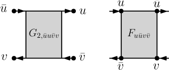
Figure 1: Graphical representation of the 4-point functions

The fully reducible vertex $F$ is defined as the amputated, connected four-point function:

$$F_{u\bar{u}v\bar{v}}\equiv G_{\bar{a}u}^{-1}G_{\bar{u}a}^{-1}G_{2,\bar{a}a\bar{b}b}G_{\bar{b}v}^{-1}G_{\bar{v}b}^{-1}$$ (18)

$F$ contains all connected diagrams with two outgoing and two ingoing entries. We note that $G_{2}$ and $F$ are of slightly different nature: $F$ is of the “vertex” type (it is amputated, i.e. its external points correspond to bare vertices), while $G_{2}$ is a “correlator” (it is not amputated, i.e. its external points correspond to propagator ends). In diagrams, “vertices” can only be connected to “correlators”, and reciprocally. $G_{2}$ and $F$ are shown graphically in Fig. 1.

We next define the irreducible vertex in channel $r$, $\Gamma^{r}$, where $r=\mathrm{ph},\overline{\mathrm{ph}},\mathrm{pp}$. The irreducible vertex in the particle-hole channel, $\Gamma^{\mathrm{ph}}$ (resp. irreducible vertex in the horizontal particle-hole channel, $\Gamma^{\mathrm{\overline{ph}}}$), contains all diagrams that do not fall apart if two horizontal (resp. vertical) counterpropagating propagators are cut open. Similarly, the irreducible vertex in the particle-particle channel, $\Gamma^{\mathrm{pp}}$, contains all diagrams which do not fall apart when two propagators going in the same direction are cut open.

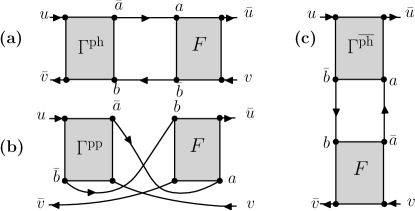
Figure 2: Graphical representation of the reducible vertex $\Phi^{r}$ in the three channels. (a) $\Phi^{\mathrm{ph}}$ (b) $\Phi^{\mathrm{pp}}$ (c) $\Phi^{\overline{\mathrm{ph}}}$.

These diagrammatic definitions imply that $F$ and $\Gamma^{r}$ are related by the Bethe-Salpether equation:

$$F_{u\bar{u}v\bar{v}} = \Gamma_{u\bar{u}v\bar{v}}^{r}+\Phi_{u\bar{u}v\bar{v}}^{r}$$ (19)

where

$$\Phi_{u\bar{u}v\bar{v}}^{\mathrm{ph}} =\Gamma_{u\bar{a}b\bar{v}}^{\mathrm{ph}}G_{a\bar{a}}G_{b\bar{b}}F_{a\bar{u}v\bar{b}}$$ (20a)

$$\Phi_{u\bar{u}v\bar{v}}^{\overline{\mathrm{ph}}} =\Gamma_{u\bar{u}a\bar{b}}^{\mathrm{\overline{ph}}}G_{a\bar{a}}G_{b\bar{b}}F_{b\bar{a}v\bar{v}}$$ (20b)

$$\Phi_{u\bar{u}v\bar{v}}^{\mathrm{pp}} =\Gamma_{u\bar{a}v\bar{b}}^{\mathrm{pp}}G_{a\bar{a}}G_{b\bar{b}}F_{b\bar{u}a\bar{v}}$$ (20c)

The function $\Phi^{r}$ is called the “reducible vertex in channel $r$”. These relations are illustrated in Fig. 2.

Next, we define the (interacting and “open”) bubble in channel $r$, $\chi^{r}$, as:

$$\chi_{\bar{u}u\bar{v}v}^{\mathrm{ph}} \equiv G_{u\bar{u}}G_{v\bar{v}}$$ (21a)

$$\chi_{\bar{u}u\bar{v}v}^{\mathrm{\overline{ph}}} \equiv G_{v\bar{u}}G_{u\bar{v}}$$ (21b)

$$\chi_{\bar{u}u\bar{v}v}^{\mathrm{pp}} \equiv G_{v\bar{u}}G_{u\bar{v}}$$ (21c)

We now introduce a change of notation to unify the expressions (20a-20b-20c). For “vertex” functions $V_{u\bar{u}v\bar{v}}$ like $F$, $\Gamma^{r}$ and $\Phi^{r}$, we introduce the following three hatted functions $\hat{V}_{r}$:

$$\hat{V}_{\mathrm{ph},u\bar{v},\bar{u}v} \equiv V_{u\bar{u}v\bar{v}}$$ (22a)

$$\hat{V}_{\overline{\mathrm{ph}},\bar{u}u,\bar{v}v} \equiv V_{u\bar{u}v\bar{v}}$$ (22b)

$$\hat{V}_{\mathrm{pp},uv,\bar{u}\bar{v}} \equiv V_{u\bar{u}v\bar{v}}$$ (22c)

Here, the subscript $r$ defines the pairing of the four indices. This is to be distinguished from superscripts (like in $\Phi^{r}$), which denote an intrinsic dependence on the channel. Thus $\hat{F}_{r}$, which is “$F$ in the $r$ notation”, depends on $r$ (whereas $F$ does not intrinsically depend on $r$). $\hat{\Phi}_{r^{\prime}}^{r}$ is “$\Phi^{r}$ in the $r^{\prime}$ notation”, it depends on $r^{\prime}$ (subscript) through the notation and intrinsically on $r$ (superscript). For “correlator” functions $C_{\bar{u}u\bar{v}v}$ (like $G_{2}$ and $\chi^{r}$), likewise, we introduce the following three hatted functions:

$$\hat{C}_{\mathrm{ph},\bar{u}v,u\bar{v}} \equiv C_{\bar{u}u\bar{v}v}$$ (23a)

$$\hat{C}_{\overline{\mathrm{ph}},\bar{v}v,\bar{u}u} \equiv C_{\bar{u}u\bar{v}v}$$ (23b)

$$\hat{C}_{\mathrm{pp},\bar{u}\bar{v},uv} \equiv C_{\bar{u}u\bar{v}v}$$ (23c)

With these notations, Eqs (20a-20b-20c) become a simple matrix product:

$$\hat{\Phi}_{r,\alpha\beta}^{r}\equiv\hat{\Gamma}_{r,\alpha\gamma}^{r}\hat{\chi}_{r,\gamma\delta}^{r}\hat{F}_{r\delta\beta}$$ (24)

Here, Greek indices denote the channel-dependent combination of two fermionic indices. They only make sense with a subscript $r$ to specify which pairing of indices is chosen.

We also note (see Appendix B for a proof) for further reference that we have, for all $r$:

$$\hat{G}_{2}=\hat{\chi}^{r}\hat{F}\hat{\chi}^{r}$$ (25)

The passage from the notation in channel $r$ to the notation in channel $r^{\prime}$ is performed via a tensor $\zeta_{\alpha\beta,\gamma\delta}^{r^{\prime}r}$ defined by the following transformation of “correlators”:

$$\hat{C}_{r^{\prime},\alpha\beta}=\zeta_{\alpha\beta,\gamma\delta}^{r^{\prime}r}\hat{C}_{r,\gamma\delta}$$ (26)

Here, we do not sum over $r$ and $r^{\prime}$. Some basic properties of this tensor are summarized in Appendix A. We further note that the trace of two operators which do not intrinsically depend on $r$ does not depend on the choice of notation, i.e.

$$\mathrm{Tr}\hat{C}\hat{V}=\hat{C}_{r,\alpha\beta}\hat{V}_{r,\beta\alpha}=\hat{C}_{r^{\prime},\gamma\delta}\hat{V}_{r^{\prime},\delta\gamma}$$ (27)

The transformation from $r$ notation to $r^{\prime}$ notation for vertex functions follows from this property:

$$\hat{V}_{r^{\prime},\alpha\beta}=\zeta_{\delta\gamma,\beta\alpha}^{rr^{\prime}}\hat{V}_{r,\gamma\delta}$$ (28)

In the above expressions, Einstein summation is performed only on the Greek indices. For the same reason as above, the inverse of correlators transform like vertex functions.

The Bethe-Salpether equation Eq. (19) can now be formally inverted. For all $r$’s, we have:

$$\hat{\Gamma}_{r}^{r}=\hat{F}_{r}(\hat{\mathbf{1}}+\hat{\chi}_{r}^{r}\hat{F}_{r})^{-1}$$ (29)

where inversion is performed in the space of Greek indices.

Finally, we define the fully irreducible vertex $\Lambda$. It contains all diagrams that are irreducible in the ph, $\overline{\mathrm{ph}}$ and pp channels. It thus obeys the relation:

$$F=\Lambda+\sum_{r}\Phi^{r}$$ (30)

Combining (19) and (30) yields:

$$\Gamma^{r}=\Lambda+\sum_{r^{\prime}\neq r}\Phi^{r^{\prime}}$$ (31)

The parquet equations are obtained by using the definition of $\Phi^{r}$, Eq. (24), and replacing $\Gamma^{r}$ and $F$ using (30) and (31):

$$\hat{\Phi}_{r}^{r}=\left(\hat{\Lambda}_{r}+\sum_{r^{\prime}\neq r}\hat{\Phi}_{r}^{r^{\prime}}\right)\hat{\chi}_{r}^{r}\left(\hat{\Lambda}_{r}+\sum_{r^{\prime}}\hat{\Phi}_{r}^{r^{\prime}}\right)$$ (32)

The parquet equations relate $\Lambda$ and $\Phi^{r}$ (at fixed $\chi^{r}$ i.e. fixed $G$), and thus [through Eqs(30-25)] $\Lambda$ to $G_{2}$. They couple the three channels (the passage from $\hat{\Phi}_{r}^{r}$ to $\hat{\Phi}_{r^{\prime}}^{r}$ is given by Eq.(26)). Conversely, the inverse parquet equations consist in computing $\Gamma^{r}$ and $\Phi^{r}$ from a given $G_{2}$ or $F$ [via Eq. (29) and (19)], and eventually [through (30)] $\Lambda$. They do not couple the three channels and are as such much easier to solve than the direct parquet equations.

The first contribution to $\Lambda$ is the bare interaction $U$. It is thus natural to define the correction of $\Lambda$ beyond $U$ as:

$$\delta\Lambda\equiv\Lambda-U$$ (33)

The lowest-order diagram of $\delta\Lambda$ is of order $U^{4}$. It is shown in Fig. 3, right panel.

One can now observe that the parquet equations formally relate the bare interactions $U$, the nontrivial contribution to the fully irreducible vertex, $\delta\Lambda$, and the (fully reducible) two-particle correlator $G_{2}$ (the functions $\Gamma^{r}$ and $\Phi^{r}$ can be regarded as by-standers). In that sense, they are analogous to the Dyson equations, which relate the bare correlator $G_{0}$, the irreducible contribution or self-energy $\Sigma$ and the (full) one-particle correlator $G$.

We note that in a single-orbital context, all the above-mentioned four-point functions depend on three momenta and three frequencies in the time- and space-translation invariant case, as well as orbital and spin indices, e.g.

$$\Lambda_{\sigma_{1}\sigma_{2}\sigma_{3}\sigma_{4}}(\mathbf{k},\mathbf{k}^{\prime},\mathbf{q},i\omega,i\omega^{\prime},i\Omega)$$

Further simplifications of the spin structure arise in SU(2) invariant problems (see e.g. Ref. Rohringer, 2013 for more details).

II.3 Four-particle irreducible formalism

Here, we introduce (subsection II.3.1) the Legendre transform of $\Gamma_{2}[G,U]$ with respect to the quartic sources, as well as its irreducible part $\mathcal{K}_{4}$ and its properties. We then show that the approximation $\mathcal{K}_{4}=0$ corresponds to the parquet approximation (subsection II.3.3), and finally prove that approximations on $\mathcal{K}_{4}$ preserve the consistency of the self-energy given as the derivative as the Luttinger-Ward functional or by the Schwinger-Dyson equation (subsection II.3.4).

II.3.1 Legendre transformation

We define the Legendre transform of $\Gamma_{2}$ with respect to $U$:

$$\Gamma_{4}[G,G_{2}]\equiv\Gamma_{2}[G,U]+\frac{1}{2}\hat{U}_{r,\alpha\beta}\hat{G}_{2,r,\beta\alpha}^{\mathrm{nc}}$$ (34)

$\Gamma_{4}$ is a functional of $G$ and $G_{2}$ (or equivalently of $G$ and $F$ via (25)) because $U$ is a functional of $G$ and $G_{2}$ through the relation:

$$G_{2,\bar{u}u\bar{v}v}^{\mathrm{nc}}[G,U]=-2\frac{\partial\Gamma_{2}}{\partial U_{u\bar{u}v\bar{v}}}\Bigg{|}_{G}$$ (35)

which follows from Eq. (5) and the properties of the Legendre transform. Note that the second term in the definition of $\Gamma_{4}$ does not depend on $r$ due to Eq. (27). The passage from a functional of the bare interaction $U$ to a functional of the $G_{2}$ (or $F$) has first been proposed in Ref. de Dominicis and Martin, 1964, and is also investigated in Ref. Van Leeuwen et al., 2006.

$\Gamma_{4}$ is the entropy of the system, up to a minus sign and a shift of the source $J-t\leftarrow J$ (where $t_{\bar{u}v}$ is the hopping integral in the quadratic part of the Hamiltonian $H$ corresponding to the action defined in Eq.(1)). Indeed, Eqs (7-34) give the relation:

$$T\Omega=\langle H\rangle-T(-\Gamma_{4})$$ (36)

where $T$ is the temperature.

Finally, from Eq. (34) and (5) follows the reciprocity relation:

$$\frac{1}{2}\hat{U}_{r,\alpha\beta}=\frac{\partial\Gamma_{4}}{\partial\hat{G}_{2,r,\beta\alpha}}\Bigg{|}_{G}$$ (37)

Following Ref de Dominicis and Martin, 1964, we define the following functional:

$$\mathcal{K}_{4}[G,G_{2}]\equiv\Phi_{\mathrm{LW}}[G,U]+\frac{1}{2}\hat{U}_{r,\alpha\beta}\hat{G}_{2,r,\beta\alpha}^{\mathrm{nc}}$$

$$\;\;\;\;\;+\frac{1}{2}\hat{F}_{r,\alpha\beta}\hat{G}_{2,r,\beta\alpha}-\frac{1}{2}\sum_{r}\Theta^{r}[G,G_{2}]$$ (38)

with

$$\Theta^{r}[G,G_{2}]\equiv$$ (39)

$$-\mathrm{Tr}\left[\ln\left(\hat{\mathbf{1}}+\hat{G}_{2,r}\left(\hat{\chi}_{r}^{r}\right)^{-1}\right)-\hat{G}_{2,r}\left(\hat{\chi}_{r}^{r}\right)^{-1}\right]$$

Thus, using Eqs (8) and (38) in Eq (34), $\Gamma_{4}$ can be written as:

$$\Gamma_{4}[G,G_{2}]=\Gamma_{2,0}[G]-\frac{1}{2}\hat{F}_{r,\alpha\beta}\hat{G}_{2,r,\beta\alpha}$$

$$\;+\frac{1}{2}\sum_{r}\Theta^{r}[G,G_{2}]+\mathcal{K}_{4}[G,G_{2}]$$ (40)

which highlights the dependence of $\Gamma_{4}$ on $G$ and $G_{2}$, and its decomposition into explicit terms (the first three terms) and a nontrivial term, $\mathcal{K}_{4}$.

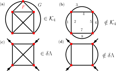
Figure 3: (a) simplest diagram of $\mathcal{K}_{4}$ (b) an example of 4-particle-reducible diagram (c) simplest diagram of $\delta\Lambda$ (d) an example of reducible 4-leg diagram. Lines denote $G$, while red squares denote $F$.

This definition of $\mathcal{K}_{4}$ ensures that $\mathcal{K}_{4}$ can be represented diagrammatically by the set of all four-particle-irreducible (4PI) diagrams, as shown in Ref. de Dominicis and Martin, 1964 in the case of bosonic fields. A diagram is said to be 4PI if for any set of four lines whose cutting leads to the separation of the diagram into two disconnected pieces, one and only one of the pieces is a simple four-leg vertex $F$. The lowest-order diagram of $\mathcal{K}_{4}$ is shown in Fig. 3(a). In Fig. 3 (b), for instance, cutting lines 3,4, 7 and 8 leads to the separation of the diagram into two disconnected pieces, none of which is a simple four-leg vertex $F$; therefore, this diagram is not 4PI.

Moreover, with definition (38), we are to show (in the next subsection) that the fully irreducible vertex $\Lambda$ (or $\delta\Lambda$) derives from $\mathcal{K}_{4}$:

$$\delta\hat{\Lambda}_{r,\alpha\beta}=-2\frac{\partial\mathcal{K}_{4}[G,G_{2}]}{\partial\hat{G}_{2,r,\beta\alpha}}\Bigg{|}_{G}$$ (41)

This is illustrated in Figure 3(c), which corresponds to the graphical derivative of the diagram of panel (a) of 3. This property can be used to devise various approximations at the 4PI level, as will be illustrated in sections II.3.3 and II.4.

Eq. (41) remarkably parallels Eq. (12) of the previous section. At the 2PI level, the stationarity of $\Gamma_{2}$ [Eq (10)] is equivalent to the fulfillment of Dyson’s equation [Eq(11)] between $G_{0}$, $G$, and $\Sigma$, the derivative of the 2PI functional, $\Phi_{\mathrm{LW}}$. Similarly, at the 4PI level, the stationarity of $\Gamma_{4}$ [Eq. (37)] is equivalent to the fulfillment of the parquet equations between $U$, $G_{2}$ and $\delta\Lambda$, the derivative of the 4PI functional $\mathcal{K}_{4}$.

II.3.2 Proof of Eq. (41)

Starting from Eq.(37), we use Eqs (34)-(40) as well as the property (deduced from Eq.(26)):

$$\frac{\partial\hat{G}_{2,r^{\prime},\kappa\eta}}{\partial\hat{G}_{2,r,\beta\alpha}}=\zeta_{\kappa\eta,\beta\alpha}^{r^{\prime}r}$$ (42)

and we remember that $F$ is just the amputated $G_{2}$ (Eq.(18), i.e the “$FG_{2}$” term contains two $G_{2}$’s at fixed $G$), to write:

$$\frac{1}{2}\hat{U}_{r,\alpha\beta}=\frac{\partial\mathcal{K}_{4}}{\partial\hat{G}_{2,r,\beta\alpha}}\Big{|}_{G}-\hat{F}_{r,\alpha\beta}$$

$$+\frac{1}{2}\sum_{r^{\prime}}\zeta_{\kappa\eta,\beta\alpha}^{r^{\prime}r}\frac{\partial\Theta^{r^{\prime}}[G,G_{2}]}{\partial\hat{G}_{2,r^{\prime},\kappa\eta}}$$ (43)

Using the chain rule and Eqs. (25-29), the last term evaluates to:

$$\frac{\partial\Theta^{r}[G,G_{2}]}{\partial\hat{G}_{2,r,\kappa\eta}}$$

$$=-\left[\left(\hat{\chi}_{r}^{r}\right)^{-1}\left(\hat{\mathbf{1}}+\hat{G}_{2}\left(\hat{\chi}_{r}^{r}\right)^{-1}\right)^{-1}-\left(\hat{\chi}_{r}^{r}\right)^{-1}\right]_{\eta\kappa}$$

$$=-\left[\left(\hat{\chi}_{r}^{r}\right)^{-1}-\left(\hat{\chi}_{r}^{r}\right)^{-1}\left(\hat{\mathbf{1}}+\hat{G}_{2,r}\left(\hat{\chi}_{r}^{r}\right)^{-1}\right)\right]_{\eta\alpha}$$

$$\;\;\;\;\times\left[\hat{\mathbf{1}}+\hat{G}_{2,r}\left(\hat{\chi}_{r}^{r}\right)^{-1}\right]_{\alpha\kappa}^{-1}$$

$$=-\left[-\left(\hat{\chi}_{r}^{r}\right)^{-1}\hat{G}_{2,r}\left(\hat{\chi}_{r}^{r}\right)^{-1}\right]_{\eta\alpha}\left[\hat{\mathbf{1}}+\hat{G}_{2,r}\left(\hat{\chi}_{r}^{r}\right)^{-1}\right]_{\alpha\kappa}^{-1}$$

$$=\hat{F}_{r,\eta\alpha}\left(\hat{\mathbf{1}}+\hat{\chi}_{r}^{r}\hat{F}_{r}\right)_{\alpha\kappa}^{-1}$$

$$=\hat{\Gamma}_{r,\eta\kappa}^{r}$$ (44)

Hence, using Eqs. (19-30), we find, using Eq. (28) and multiplying (43) by 2:

$$\hat{U}_{r,\alpha\beta} = 2\frac{\partial\mathcal{K}_{4}}{\partial\hat{G}_{2,r,\beta\alpha}}-2\hat{F}_{r,\alpha\beta}+\sum_{r^{\prime}}\zeta_{\kappa\eta,\beta\alpha}^{r^{\prime}r}\hat{\Gamma}_{r^{\prime},\eta\kappa}^{r^{\prime}}$$

$$= 2\frac{\partial\mathcal{K}_{4}}{\partial\hat{G}_{2,r,\beta\alpha}}-2\hat{F}_{r,\alpha\beta}+\sum_{r^{\prime}}\hat{\Gamma}_{r,\alpha\beta}^{r^{\prime}}$$

$$= 2\frac{\partial\mathcal{K}_{4}}{\partial\hat{G}_{2,r,\beta\alpha}}-2\hat{F}_{r,\alpha\beta}+\sum_{r^{\prime}}\left(\hat{F}_{r,\alpha\beta}-\hat{\Phi}_{r,\alpha\beta}^{r^{\prime}}\right)$$

$$= 2\frac{\partial\mathcal{K}_{4}}{\partial\hat{G}_{2,r,\beta\alpha}}+\hat{F}_{r,\alpha\beta}-\sum_{r^{\prime}}\hat{\Phi}_{r,\alpha\beta}^{r^{\prime}}$$

$$= 2\frac{\partial\mathcal{K}_{4}}{\partial\hat{G}_{2,r,\beta\alpha}}+\hat{\Lambda}_{r,\alpha\beta}$$ (45b)

In the last step, we have used Eq. (30). By identification with Eq. (33), we find the final result, Eq. (41).

II.3.3 The parquet approximation: $\mathcal{K}_{4}=0$

The most trivial approximation of $\mathcal{K}_{4}$, namely

$$\mathcal{K}_{4}^{\mathrm{parquet\,app.}}=0$$ (46)

corresponds to the parquet approximation. Indeed, Eq.(46), combined with Eqs. (33-41), leads to

$$\Lambda^{\mathrm{parquet\;app.}}=U$$ (47)

By construction, this approximation is limited to the weak-coupling regime since it neglects higher order terms. It has been recently applied to the Hubbard modelYang et al. (2009). We note that an alternative functional view on the parquet approximation is proposed in Ref. Janis, 1998.

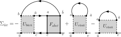
Figure 4: Schwinger-Dyson expression of the self-energy.

II.3.4 Consistency of the self-energy

Any approximation of $\mathcal{K}_{4}[G,G_{2}]$ results in (i) an approximate irreducible vertex $\delta\Lambda$ and, via the parquet equations, approximate fully reducible vertex $F$ and (ii) an approximate Luttinger-Ward functional [via. Eq. (38)].

From here, there are a priori two ways of computing the self-energy. The first way is compute $\Sigma$ as the derivative of $\Phi_{\mathrm{LW}}$ with respect to $G$ [Eq. (12)]. The second one is to use the Schwinger-Dyson equation, an exact expression giving $\Sigma$ as a function of $G$, $F$ and $U$ and illustrated in Fig. 4:

$$\Sigma_{\bar{u}v}=-U_{b\bar{a}c\bar{u}}G_{a\bar{a}}G_{c\bar{c}}G_{b\bar{b}}F_{a\bar{b}v\bar{c}}+U_{v\bar{u}a\bar{a}}G_{a\bar{a}}-U_{v\bar{a}a\bar{u}}G_{a\bar{a}}$$ (48)

The last two terms correspond to the Hartree and Fock terms, respectively.

We prove in Appendix C that provided the approximation on $\mathcal{K}_{4}[G,G_{2}]$ preserves its homogeneity properties, both ways of computing the self-energy are equivalent.

In the next subsection, we introduce, instead of the simple approximation (46), an atomic approximation of $\mathcal{K}_{4}$.

II.4 A quadruply irreducible local expansion: QUADRILEX

II.4.1 A local expansion of the 4PI functional

Similarly to DMFT, we propose to approximate the 4PI functional by the atomic limit (and later by a cluster method):

$$\mathcal{K}_{4}^{\mathrm{QUADRILEX}}[G_{\mathbf{R}_{1}\mathbf{R}_{2}},G_{2,\mathbf{R}_{1}\mathbf{R}_{2}\mathbf{R}_{3}\mathbf{R}_{4}}]$$

$$\equiv\sum_{\mathbf{R}}\mathcal{K}_{4}[G_{\mathbf{RR}},G_{2,\mathbf{RRRR}}]$$ (49)

To solve Eq. (49), we propose to follow a similar procedure as the one used in DMFT (see subsection II.1.2), by replacing $\Phi_{\mathrm{LW}}$ by $\mathcal{K}_{4}$:

First, we introduce the following model:

$$S_{\mathrm{imp}}^{\mathrm{QUADRILEX}} =$$ (50)

$$-\iint_{\tau\tau^{\prime}} \sum_{\sigma\sigma^{\prime}}\bar{c}_{\tau\sigma}\left[\mathcal{G}^{-1}(\tau-\tau^{\prime})\right]_{\sigma\sigma^{\prime}}c_{\tau^{\prime}\sigma^{\prime}}$$

$$+\frac{1}{2}\iiiint_{\begin{subarray}{c}\tau_{1}\tau_{2}\\ \tau_{3}\tau_{4}\end{subarray}} \sum_{\begin{subarray}{c}\sigma_{1}\sigma_{2}\\ \sigma_{3}\sigma_{4}\end{subarray}}\mathcal{U}_{\sigma_{1}\sigma_{2}\sigma_{3}\sigma_{4}}^{\tau_{1},\tau_{2},\tau_{3},\tau_{4}}\bar{c}_{\tau_{1}\sigma_{1}}c_{\tau_{2}\sigma_{2}}\bar{c}_{\tau_{3}\sigma_{3}}c_{\tau_{4}\sigma_{4}}$$

This action describes an impurity embedded in a noninteracting bath described by the field $\mathcal{G}$ and with dynamical interactions $\mathcal{U}$ with three independent times. Its functional $\mathcal{K}_{4}[G,G_{2}]$ is the same as the summand of the right-hand side of Eq. (49), and does not depend on the non-interacting propagator $\mathcal{G}(i\omega)$ and bare interaction $\mathcal{U}(i\omega,i\omega^{\prime},i\Omega)$.

Second, we assume that one can adjust the non-interacting propagator $\mathcal{G}$ and bare interaction $\mathcal{U}$ of the auxiliary model such that

$$G_{\mathrm{imp}}[\mathcal{G},\mathcal{U}](i\omega) = G_{\mathbf{RR}}(i\omega)$$ (51a)

$$G_{\mathrm{2,imp}}[\mathcal{G},\mathcal{U}](i\omega,i\omega^{\prime},i\Omega) = G_{2,\mathbf{RRRR}}(i\omega,i\omega^{\prime},i\Omega)$$

$\mathcal{G}$ and $\mathcal{U}$ can be thought of as Lagrange multipliers to enforce the two above constraints.

Finally, if we solve Eqs (51a-LABEL:eq:G2_self_consistency), then

$$\mathcal{K}_{4}^{\mathrm{imp}}[G_{\mathrm{imp}},G_{2,\mathrm{imp}}]=\mathcal{K}_{4}[G_{\mathbf{RR}},G_{2,\mathbf{RRRR}}]$$

and therefore Eqs. (41)-(49) imply that

$$\delta\Lambda(\mathbf{k},\mathbf{k}^{\prime},\mathbf{q},i\omega,i\omega^{\prime},i\Omega)=\delta\Lambda_{\mathrm{imp}}(i\omega,i\omega^{\prime},i\Omega)$$ (52)

For simplicity, we will henceforth use the following shorthand notation for 4-leg functions on the lattice:

$$X_{\mathrm{latt}}\equiv X_{\sigma_{1}\sigma_{2}\sigma_{3}\sigma_{4}}(\mathbf{k},\mathbf{k^{\prime}},\mathbf{q},i\omega,i\omega^{\prime},i\Omega)$$ (53)

We point out that while DMFT is the approximation of $\Phi_{\mathrm{LW}}[G,U]$, which depends on one full correlator, $G$, and has correspondingly one “dynamical bath” $\mathcal{G}$, QUADRILEX, an approximation of $\mathcal{K}_{4}[G,G_{2}]$, which depends on two full correlators, $G$ and $G_{2}$, involves two dynamical mean fields $\mathcal{G}$ and $\mathcal{U}$ corresponding to two constraints, Eqs (51a-LABEL:eq:G2_self_consistency).

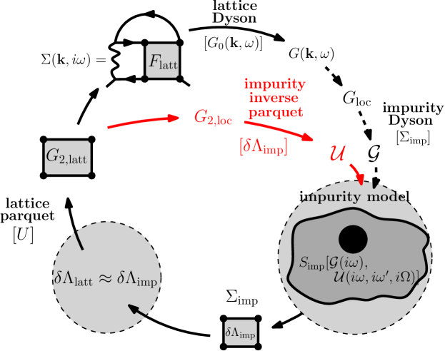
Figure 5: (color online) The QUADRILEX loop. The parts in black correspond to the D$\Gamma$A in the parquet version (the dashed line shows how D$\Gamma$A proposes to update the Weiss field $\mathcal{G}(i\omega)$). The parts in red correspond to the additional steps necessary to update the bare impurity vertex $\mathcal{U}(i\omega,i\omega^{\prime},i\Omega)$. For $\Sigma$ we show only the terms beyond Hartree-Fock. The terms in square brackets denote the fixed terms in the solution of the Dyson/parquet equations.

II.4.2 QUADRILEX construction

In dynamical mean field theory, the constraint Eq. (51a) is used together with the Dyson equation to determine the self-consistent bath $\mathcal{G}$ from a given impurity self-energy $\Sigma_{\mathrm{imp}}$. This is done as follows:

(i) the lattice self-energy $\Sigma(\mathbf{k},i\omega)$ is approximated by the impurity self-energy $\Sigma_{\mathrm{imp}}$;

(ii) $\Sigma(\mathbf{k},i\omega)$ is plugged into the lattice Dyson equation (at fixed $G_{0}(\mathbf{k},i\omega)$) to get $G(\mathbf{k},i\omega)$, which is summed over the Brillouin zone to get $G_{\mathrm{loc}}(i\omega)$;

(iii) The impurity Dyson equation is inverted to get $\mathcal{G}$ from $\Sigma_{\mathrm{imp}}$ and $G_{\mathrm{loc}}$.

In QUADRILEX, the same procedure is applied to get the retarded interactions $\mathcal{U}(i\omega,i\omega^{\prime},i\Omega)$ from a given impurity fully irreducible vertex $\delta\Lambda_{\mathrm{imp}}(i\omega,i\omega^{\prime},i\Omega)$. Instead of the Dyson equations, one uses the parquet equations which relate the bare interactions, the fully irreducible vertex and the fully reducible vertex (see section II.2):

(i) the lattice fully irreducible vertex $\delta\Lambda_{\mathrm{latt}}$ is approximated by the impurity fully irreducible vertex $\delta\Lambda_{\mathrm{imp}}(i\omega,i\omega^{\prime},i\Omega)$

(ii) $\delta\Lambda_{\mathrm{latt}}$ is plugged into the lattice parquet equations (at fixed lattice bare interactions $\hat{U}$) to get $G_{2,\mathrm{latt}}$, which is summed over the Brillouin zone to get $G_{2,\mathrm{loc}}(i\omega,i\omega^{\prime},i\Omega)$

(iii) The impurity parquet equations are inverted to get $\mathcal{U}(i\omega,i\omega^{\prime},i\Omega)$ from $\delta\Lambda_{\mathrm{imp}}$ and $G_{\mathrm{2,loc}}$.

This construction is remarkable in that the impurity model’s bare interaction $\mathcal{U}_{\sigma_{1}\sigma_{2}\sigma_{3}\sigma_{4}}(i\omega,i\omega^{\prime},i\Omega)$ is a priori different from the lattice’s bare interaction $U_{\sigma_{1}\sigma_{2}\sigma_{3}\sigma_{4}}$. The deviation of $\mathcal{U}_{\sigma_{1}\sigma_{2}\sigma_{3}\sigma_{4}}(i\omega,i\omega^{\prime},i\Omega)$ from $U_{\sigma_{1}\sigma_{2}\sigma_{3}\sigma_{4}}$, both from the point of view of the frequency dependence and from the point of view of the spin structure, is an interesting topic of investigation. We discuss this in more detail in section III.

II.4.3 Self-consistent loop

Like DMFT, the equations of section II.4.1 may be solved in an iterative way. We propose the following self-consistent loop:

1. Start with a given $\mathcal{U}(i\omega,i\omega^{\prime},\Omega)$ and $\mathcal{G}(i\omega)$ and solve the corresponding impurity model, Eq. (50), for $G_{\mathrm{imp}}$ and $G_{\mathrm{2,imp}}$, from which one can (through the impurity Dyson and inverse parquet equations) compute $\Sigma_{\mathrm{imp}}(i\omega)$ and $\delta\Lambda_{\mathrm{imp}}(i\omega,i\omega^{\prime},i\Omega)$;

2. Use Eq. (52) to get a starting point for a parquet solver on the lattice. This yields $G_{2,\mathrm{latt}}$;

3. Use $G_{2}$ (or equivalently $F$) to compute $\Sigma(\mathbf{k},i\omega)$ via the Schwinger-Dyson equation [Eq. (48)], and then $G(\mathbf{k},i\omega)$ via the Dyson equation;

4. Compute the new bath $\mathcal{G}$ and interactions $\mathcal{U}$:

   1. Take the local part of $G(\mathbf{k},i\omega)$ to compute the new Weiss field as (black part in Fig. 5):

      $$\mathcal{G}^{-1}=G_{\mathrm{loc}}^{-1}+\Sigma_{\mathrm{imp}}$$ (54)

   2. Take the local part of $G_{2,\mathrm{latt}}$, $G_{2,\mathrm{loc}}$ and use the inverse parquet equations (at fixed $G_{2,\mathrm{loc}}$ and $\delta\Lambda_{\mathrm{imp}}$) to compute $\mathcal{U}(i\omega,i\omega^{\prime},i\Omega)$ (red part), i.e compute $\Lambda_{\mathrm{imp}}^{{}^{\prime}}$ from the inverse parquet (the prime emphasizes the fact that $\Lambda_{\mathrm{imp}}^{{}^{\prime}}$ is obtained after using lattice quantities, as opposed to $\delta\Lambda_{\mathrm{imp}}$ which is computed directly from the impurity model) and get $\mathcal{U}$ as:

      $$\mathcal{U}=\Lambda_{\mathrm{imp}}^{{}^{\prime}}-\delta\Lambda_{\mathrm{imp}}$$ (55)

5. Go back to step 1. until convergence.

This self-consistent cycle is summarized in Fig. 5. The dynamical vertex approximation (D$\Gamma$A in its parquet version) corresponds to the black parts, namely the computation of $G_{2,\mathrm{latt}}$ from a given impurity vertex $\delta\Lambda_{\mathrm{imp}}(i\omega,i\omega^{\prime},i\Omega)$. The computation of the updated impurity bare interaction is shown in red.

III Discussion

III.1 A dynamical vertex approximation, and beyond

The local approximation of the lattice vertex, Eq. (52), is the essence of the dynamical vertex approximation (D$\Gamma$AToschi et al. (2007); Held (2014)). In fact, D$\Gamma$A in its parquet version can be regarded as a one-shot realization of the 4PI formalism.

The main difference of QUADRILEX with D$\Gamma$A is that in D$\Gamma$A, the vertex $\mathcal{U}$ of the impurity model is not renormalized, namely in D$\Gamma$A, Eq. (55) becomes:

$$\mathcal{U}^{\mathrm{D\Gamma A}}(i\omega,i\omega^{\prime},i\Omega)=U$$ (56)

As will be seen in the next subsection, this condition is a priori valid only in the atomic limit. As soon as the bandwidth is finite, deviations of $\mathcal{U}$ with respect to $U$ are likely to appear.

Interestingly, the natural variable of the QUADRILEX approximation is the fully irreducible vertex $\Lambda$, which is approximated locally in the parquet version of the dynamical vertex approximation. This contrasts with the ladder version of D$\Gamma$A, where the local approximation is done at the level of the irreducible vertex in one channel, $\Gamma^{r}$. This vertex derives from another functional, $\Theta^{r}[G,G_{2}]$ [Eq.(44)]. In this variant of D$\Gamma$A, sum rules on the susceptibilities (or equivalently the asymptotic behavior of the self-energy) are violated unless some corrections (called “Moriya corrections” in the D$\Gamma$A literatureKatanin et al. (2009)) are made.

Another important consequence of our functional construction is that the QUADRILEX method can capture the feedback of long-range interactions into the impurity model. In D$\Gamma$A, this feature only appears in the solution of the lattice parquet equations (through $U$, which can in principle have a nonlocal part). One can expect nonlocal physics to be reflected by a sizable frequency dependence of the local interaction, $\mathcal{U}$. This frequency dependence can capture some nonlocal effects of nonlocal interactions such as charge-ordering phenomena, as has been observed e.g. in extended DMFTAyral et al. (2012, 2013); Huang et al. (2014).

III.2 An interpolation between atomic physics and collective-mode physics

As a local expansion of the 4PI functional, QUADRILEX allows to interpolate between the atomic limit and the limit of the parquet approximation, which can describe collective modes.

Indeed, in the atomic limit, all momentum dependences drop out and one recovers, by construction,

$$\mathcal{U}^{\mathrm{at}}(i\omega,i\omega^{\prime},i\Omega)=U$$ (57)

since the impurity’s fully irreducible vertex $\Lambda_{\mathrm{imp}}$ is the exact fully irreducible vertex of the lattice.

In the weak-coupling regime, $\Lambda_{\mathrm{imp}}$ is roughly equal to the bare interaction $U$ (the first correction is of order $U^{4}$), which corresponds to the parquet approximation. Although the precise form of the impurity’s bare interaction $\mathcal{U}_{\mathrm{imp}}(i\omega,i\omega^{\prime},i\Omega)$ in this limit is difficult to predict a priori, one may speculate that already in this limit a differentiation between the charge and the spin channel occurs. Such a differentiation has been observed within the two-particle self-consistent method (TPSCVilk et al. (1994); Vilk and Tremblay (1996, 1997); Tremblay (2011)).

III.3 Avoiding the parquet: bosonic variables

Degree of irreducibility	Functional	Full correlators	Irred. object	Bare “bath”
2PI (DMFT)	$\Phi_{\mathrm{LW}}[G,U]:$ $\Sigma=\frac{\partial\Phi_{\mathrm{LW}}}{\partial G}$	$G$	$\Sigma$	$\mathcal{G}_{i\omega}^{-1}$
2PI (EDMFT)	$\Psi[G,W,\lambda]:$ $P=-2\frac{\partial\Psi}{\partial W}$	$G$, $W$	$\Sigma$,$P$	$\mathcal{G}_{i\omega}^{-1}$, $\mathcal{U}_{i\Omega}^{-1}$
3PI (TRILEX)	$\mathcal{K}_{3}[G,W,\chi_{3}]:$ $K=-\frac{\partial\mathcal{K}_{3}}{\partial\chi_{3}}$	$\chi_{3}$, $G$, $W$	$K$	$\lambda_{i\omega,i\Omega}^{\mathrm{imp}}$, $\mathcal{G}_{i\omega}^{-1}$ , $\mathcal{U}_{i\Omega}^{-1}$
4PI (QUADRILEX)	$\mathcal{K}_{4}[G,G_{2}]:$ $\delta\Lambda=-2\frac{\partial\mathcal{K}_{4}}{\partial G_{2}}$	$G_{2}$, $G$	$\delta\Lambda$	$\mathcal{U}_{i\omega,i\omega^{\prime},i\Omega}$, $\mathcal{G}_{i\omega}^{-1}$

Table 1: Comparison of the observables for various degrees of irreducibilities. While 2PI observables are related via Dyson equations, 3PI observables are simply related by a linear equation, and 4PI observables are related by parquet equations (see text for definitions).

From a technical point of view, the present method has two difficulties:

(i) The solution of parquet equations on the lattice is still a major computational hurdle despite recent progressTam et al. (2013); Li et al. (2016). This has so far limited the range of applications of parquet-based methods such as parquet-D$\Gamma$A to very small system sizes.Valli et al. (2015)

(ii) The impurity model Eq. (50) features dynamical interactions with three independent time variables. A straightforward extension of the existing implementationsParcollet et al. (2015) of the interaction-expansion continuous-time quantum Monte-Carlo algorithmGull et al. (2011) allows to handle this type of problems. It consists in using interaction vertices depending on four time variables instead of one in the Monte-Carlo configurations. However, one cannot foretell the severity of the minus sign problem in the expansion of interaction with three independent frequencies, which could limit the practical applicability of the method. We nonetheless note that in some physical regimes, one may expect the frequency dependence of $\mathcal{U}$ to be restricted to the bosonic frequency. In this case, the hybridization expansion solver with dynamical interactions, which is sign-problem-free in the single-band, density-density case, can be usedWerner and Millis (2007).

An alternative to dealing with the complexity of the four-fermion interaction is provided by another class of methods also inspired by DMFT, but relying on the introduction of auxiliary bosonic degrees of freedom guided by physical insight into the instabilities of the system. These methods include the extended DMFT method (EDMFTSengupta and Georges (1995); Kajueter (1996); Si and Smith (1996)), the recently introduced TRILEX methodAyral and Parcollet (2015, 2016).

EDMFT is the straightforward extension of DMFT to electron-boson problems with fermionic fields (propagator $G$) and bosonic fields (propagator $W$). In this context, the 2PI functional is denoted as $\Psi[G,W,\lambda]$, where $\lambda$ is the bare electron-boson coupling. All the fermionic equations of DMFT can be transposed for bosonic variables, namely for the bosonic propagator $W$, the bosonic self-energy $P$ and the bosonic free propagator $W_{0}$.

The TRILEX method takes EDMFT from the 2PI level (and its functional $\Psi[G,W,\lambda]$) to the 3PI level and its functional $\mathcal{K}_{3}[G,W,\chi_{3}]$, where $\chi_{3}$ is now the fully three-point electron-boson correlation function. Similarly to DMFT and QUADRILEX, it consists in a local expansion of a functional, which is, in the case of TRILEX, the 3PI functional $\mathcal{K}_{3}$.

In this approach, the impurity problem has three “Lagrange multipliers” or dynamical baths, $\mathcal{G}$, $\mathcal{W}$ and $\lambda^{\mathrm{imp}}$ to satisfy the three constaints on $G_{\mathrm{imp}}$, $W_{\mathrm{imp}}$ and $\chi_{3,\mathrm{imp}}$. The atomic approximation of $\mathcal{K}_{3}$ results in a local approximation of the irreducible vertex

$$K(\mathbf{k},\mathbf{q},i\omega,i\Omega)=K_{\mathrm{imp}}(i\omega,i\Omega)$$

Table 1 summarizes the various methods. Each method corresponds to the atomic approximation of the nontrivial part ($\Phi_{\mathrm{LW}}[G,U]$, $\Psi[G,W,\lambda]$, $\mathcal{K}_{3}[G,W,\chi_{3}]$ or $\mathcal{K}_{4}[G,G_{2}]$ respectively) of a functional ($\Gamma_{2}[G,U]$, $\Gamma_{2}[G,W,\lambda]$, $\Gamma_{3}[G,W,\chi_{3}]$ or $\Gamma_{4}[G,G_{2}]$ respectively). Stationarity of this functional is equivalent to the fulfillment of “boldification” equations (fermionic or bosonic Dyson equation, simple linear relation (Eq. 18 in Ref. Ayral and Parcollet, 2016), or parquet equations, respectively) relating three kinds of objects. We will call these objects the “full” or bold objects (the fermionic or bosonic Green’s functions $G$ and $W$, connected three- or four-point functions $\chi_{3}$ and $G_{2}$, respectively), the “irreducible” objects (the self-energy $\Sigma$, the polarization $P$, the irreducible three-leg vertex $K$ or fully irreducible four-leg vertex $\delta\Lambda$) and the “bare” objects ($G_{0}^{-1}$, $W_{0}^{-1}$, $\lambda$ or $U$ at the lattice level, $\mathcal{G}_{i\omega}^{-1}$, $\mathcal{U}_{i\Omega}^{-1}$, $\lambda_{i\omega,i\Omega}^{\mathrm{imp}}$ or $\mathcal{U}_{i\omega,i\omega^{\prime},i\Omega}$ at the impurity level).

In each method, the impurity model is used to compute the irreducible objects, which are used as an approximation of the corresponding lattice irreducible object via the atomic approximation of the corresponding functional. As mentioned before, the variables of this functional are the full objects, and the atomic approximation imposes that the local components of these objects coincide with their impurity counterparts. The knowledge of the full and irreducible objects at the impurity level allows to find, through the boldification equations, the third object, namely the bare object which is used as a bath or retarded interaction in the impurity model.

Other recent methods use bosonic variables to avoid the solution of parquet equations. A recent example is the dual boson methodRubtsov et al. (2012); van Loon et al. (2014); Stepanov et al. (2016): it introduces different auxiliary bosonic degrees of freedom, and relies on the solution of the same impurity model as extended DMFT (with updated baths in the self-consistent version of the method), and the subsequent resummation of a selected subclass of self-energy diagrams built with the lowest-order impurity vertices.

IV Conclusion and perspectives

In this paper, we have used the four-particle irreducible formalism to build an expansion of the 4PI functional $\mathcal{K}_{4}$ around the atomic limit. This approximation implies a local approximation of the fully irreducible vertex, like in the dynamical vertex approximation (D$\Gamma$A). It maps the lattice model onto an effective local impurity model with both a dynamical field $\mathcal{G}$ and dynamical interactions $\mathcal{U}$ with three independent frequencies (contrary to D$\Gamma$A). By construction, this method extrapolates between the atomic limit at strong coupling and the description of collective modes by parquet equations at weak coupling.

This functional derivation naturally extends the DMFT idea – a local expansion of the 2PI functional – to the 4PI level and sets up a framework to understand how to generate extensions of DMFT. In particular, it gives prescriptions as to how to construct the parameters of the local auxiliary model of DMFT-like approaches. It is applicable to models with local, but also nonlocal interactions where we expect the dynamical aspect of the interactions to play an important role.

This functional construction lays the groundwork for more advanced inquiries about the preservation of conservation laws. One may speculate that going from 2PI self-consistent (“$\Phi$-derivable”) approximations to “$\mathcal{K}_{4}$-derivable” approximations endows one with better conservation properties.

The actual implementation of this method is within computational reach and work is in progress in this direction. On the one hand, the solution of lattice parquet equations is already part of the parquet-D$\Gamma$A method and has benefited from recent progress.Tam et al. (2013); Li et al. (2016) On the other hand, impurity models with dynamical, three-frequency interactions can be handled by interaction-expansion continuous-time quantum Monte-Carlo solvers, provided the sign problem is not too severe.

Appendix A Properties of the $\zeta$ tensor

The tensor $\zeta^{rr^{\prime}}$ is made of 0’s and 1’s, and obeys the relation (to be read as a matrix product in combined $(\alpha\beta)$ indices):

$$\zeta^{rr^{\prime}}\cdot\zeta^{r^{\prime}r}=\mathbf{1}$$ (58)

Indeed, for any $\hat{C}$,

$$\hat{C}_{r,\bar{\gamma}\bar{\delta}}=\zeta_{\bar{\gamma}\bar{\delta},\alpha\beta}^{rr^{\prime}}\hat{C}_{r^{\prime},\alpha\beta}=\zeta_{\bar{\gamma}\bar{\delta},\alpha\beta}^{rr^{\prime}}\zeta_{\alpha\beta,\gamma\delta}^{r^{\prime}r}\hat{C}_{r,\gamma\delta}$$

and therefore $\zeta_{\bar{\gamma}\bar{\delta},\alpha\beta}^{rr^{\prime}}\zeta_{\alpha\beta,\gamma\delta}^{r^{\prime}r}=\delta_{\bar{\gamma},\gamma}\delta_{\bar{\delta}\delta}$.

Appendix B Relation between $G_{2}$ and $F$ in channel notation

In this section, we prove Eq. (25). We have:

$$\hat{\chi}_{\mathrm{ph},\alpha\delta}^{\mathrm{ph}}\hat{F}_{\mathrm{ph},\delta\gamma}\hat{\chi}_{\mathrm{ph},\gamma\beta}^{\mathrm{ph}} =\hat{\chi}_{\mathrm{ph},\bar{a}b,a\bar{b}}^{\mathrm{ph}}\hat{F}_{\mathrm{ph},a\bar{b},\bar{v}v}\hat{\chi}_{\mathrm{ph},\bar{v}v,u\bar{u}}^{\mathrm{ph}}$$

$$=G_{a\bar{a}}G_{b\bar{b}}F_{a\bar{v}v\bar{b}}G_{u\bar{v}}G_{v\bar{u}}$$

$$=G_{2,\bar{a}u\bar{u}b}$$

$$=\hat{G}_{2,\mathrm{ph},\bar{a}b,u\bar{u}}$$

$$=\hat{G}_{2,\mathrm{ph},\alpha\beta}$$

$$\hat{\chi}_{\mathrm{\overline{ph}},\alpha\delta}^{\mathrm{\overline{ph}}}\hat{F}_{\mathrm{\mathrm{\overline{ph}}},\delta\gamma}\hat{\chi}_{\mathrm{\overline{ph}},\gamma\beta}^{\mathrm{\mathrm{\overline{ph}}}} =\hat{\chi}_{\mathrm{\overline{ph}},\bar{u}u,\bar{v}v}^{\mathrm{\overline{ph}}}\hat{F}_{\mathrm{\overline{ph}},\bar{v}v,\bar{a}a}\hat{\chi}_{\mathrm{\overline{ph}},\bar{a}a,\bar{b}b}^{\mathrm{\overline{ph}}}$$

$$=G_{u\bar{v}}G_{v\bar{u}}F_{v\bar{v}a\bar{a}}G_{a\bar{b}}G_{b\bar{a}}$$

$$=G_{2,\bar{u}u\bar{b}b}$$

$$=G_{2,\bar{b}b\bar{u}u}$$

$$=\hat{G}_{2,\overline{\mathrm{ph}},\bar{u}u,\bar{b}b}$$

$$=\hat{G}_{2,\overline{\mathrm{ph}},\alpha\beta}$$

and

$$\hat{\chi}_{\mathrm{pp},\alpha\delta}^{\mathrm{pp}}\hat{F}_{\mathrm{pp},\delta\gamma}\hat{\chi}_{\mathrm{pp},\gamma\beta}^{\mathrm{\mathrm{pp}}} =\hat{\chi}_{\mathrm{pp},\bar{u}\bar{v},uv}^{\mathrm{pp}}\hat{F}_{\mathrm{pp},uv,\bar{a}\bar{b}}\hat{\chi}_{\mathrm{pp},\bar{a}\bar{b},ab}^{\mathrm{pp}}$$

$$=G_{v\bar{u}}G_{u\bar{v}}F_{u\bar{a}v\bar{b}}G_{a\bar{b}}G_{b\bar{a}}$$

$$=G_{2,\bar{v}b\bar{u}a}$$

$$=G_{2,\bar{u}a\bar{v}b}$$

$$=\hat{G}_{2,\mathrm{pp},\bar{u}\bar{v},ab}$$

$$=\hat{G}_{2,\mathrm{pp},\alpha\beta}$$

We have used the crossing symmetry

$$G_{2,\bar{u}u\bar{v}v}=G_{2,\bar{v}v\bar{u}u}$$ (59)

for the last two equalities.

Appendix C Consistency of the Self-Energy in the 4PI formalism

Here, we show that $\Sigma$ given by the Schwinger-Dyson equation is identical to the derivative of the Luttinger-Ward functional with respect to $G$ (Eq. (12)) based on the homogeneity properties of the 4PI functional.

We first express $\Phi_{\mathrm{LW}}$ as a function of $G$, $U$ and $G_{2}$ using Eq. (38):

$$\tilde{\Phi}_{\mathrm{LW}}[G,U,G_{2}]\equiv R[G,G_{2}]-\frac{1}{2}\hat{U}_{r,\alpha\beta}\hat{G}_{2,r,\beta\alpha}^{\mathrm{nc}}$$ (60)

with

$$R[G,G_{2}]\equiv\mathcal{K}_{4}[G,G_{2}]+\frac{1}{2}\sum_{r}\Theta^{r}[G,G_{2}]$$

$$-\frac{1}{2}\left(\hat{\chi}_{r,\alpha\gamma}^{r}\right)^{-1}\hat{G}_{2,\gamma\delta}\left(\hat{\chi}_{r,\delta\beta}^{r}\right)^{-1}\hat{G}_{2,r,\beta\alpha}$$ (61)

Then, following (12), $\Sigma$ is given by:

$$\Sigma_{\bar{u}v}=\frac{\partial\tilde{\Phi}_{\mathrm{LW}}}{\partial G_{v\bar{u}}}\Bigg{|}_{U,G_{2}}+\frac{\partial\tilde{\Phi}_{\mathrm{LW}}}{\partial\hat{G}_{2,r,\alpha\beta}}\Bigg{|}_{U,G}\frac{\partial\hat{G}_{2,r,\alpha\beta}}{\partial G_{v\bar{u}}}$$

The second term evaluates to zero. Indeed, we can first, using Eqs (34) and (8), see that

$$R[G,G_{2}]=\Gamma_{4}[G,G_{2}]-\Gamma_{2,0}[G]$$ (62)

Then, using Eq. (62), the fact that $\Gamma_{2,0}$ does not depend on $G_{2}$ and Eq (37), we obtain:

$$\frac{\partial\tilde{\Phi}_{\mathrm{LW}}}{\partial\hat{G}_{2,r,\alpha\beta}}\Bigg{|}_{U,G} =\frac{\partial\Gamma_{4}}{\partial\hat{G}_{2,r,\alpha\beta}}\Bigg{|}_{U,G}-\frac{1}{2}\hat{U}_{r,\beta\alpha}=0$$ (63)

Hence:

$$\Sigma_{\bar{u}v} =\frac{\partial R}{\partial G_{v\bar{u}}}\Bigg{|}_{U,G_{2}}+\Sigma_{\bar{u}v}^{\mathrm{HF}}$$ (64)

where we have defined:

$$\Sigma_{\bar{u}v}^{\mathrm{HF}} \equiv-\frac{1}{2}\frac{\partial}{\partial G_{v\bar{u}}}\left[U_{a\bar{a}b\bar{b}}\left(-G_{a\bar{a}}G_{b\bar{b}}+G_{a\bar{b}}G_{b\bar{a}}\right)\right]$$

$$=\frac{1}{2}U_{a\bar{a}b\bar{b}}\Big{(}\delta_{av}\delta_{\bar{u}\bar{a}}G_{b\bar{b}}+G_{a\bar{a}}\delta_{vb}\delta_{\bar{u}\bar{b}}$$

$$\;\;-\delta_{va}\delta_{\bar{u}\bar{b}}G_{b\bar{a}}-G_{a\bar{b}}\delta_{vb}\delta_{\bar{u}\bar{a}}\Big{)}$$

$$=\frac{1}{2}\Big{(}U_{v\bar{u}b\bar{b}}G_{b\bar{b}}+U_{a\bar{a}v\bar{u}}G_{a\bar{a}}$$

$$\;\;-U_{v\bar{a}b\bar{u}}G_{b\bar{a}}-U_{a\bar{u}v\bar{b}}G_{a\bar{b}}\Big{)}$$

$$=U_{v\bar{u}a\bar{a}}G_{a\bar{a}}-U_{v\bar{a}a\bar{u}}G_{a\bar{a}}$$

To obtain the last line, we have used the crossing symmetry (59) and relabelled the indices. This is the Hartree-Fock term.

As for the first term of (64), it can be rewritten using the homogeneity properties of $R$. Let us first show that $R$ is the sum of homogeneous functions of the function $Y^{r}$, namely

$$R[G,G_{2}]=\sum_{r}\tilde{R}^{r}[\hat{Y}^{r}]$$ (65)

with:

$$\hat{Y}^{r}\equiv\left(\hat{\chi}^{r}\right)^{-1}\hat{G}_{2}$$ (66)

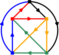
Figure 6: (color online) Homogeneity of the lowest-order diagram of $\mathcal{K}_{4}$ in $\hat{Y}^{\mathrm{pp}}$. Each colored piece stands for $\hat{Y}^{\mathrm{pp}}=(\hat{\chi}^{\mathrm{pp}})^{-1}\hat{G}_{2}=\hat{F}\hat{\chi}^{\mathrm{pp}}$.

This property follows from the homogeneity of the three terms in the definition of $R$, Eq. (61). $\mathcal{K}_{4}$ is homogeneous with respect to $Y^{r}$ in the three channels:

$$\mathcal{K}_{4}[G,G_{2}]=\tilde{\mathcal{K}}_{4}^{\mathrm{ph}}[Y^{\mathrm{ph}}]=\tilde{\mathcal{K}}_{4}^{\overline{\mathrm{ph}}}[Y^{\overline{\mathrm{ph}}}]=\tilde{\mathcal{K}}_{4}^{\mathrm{pp}}[Y^{\mathrm{pp}}]$$ (67)

The homogeneity of the lowest diagram of $\mathcal{K}_{4}$ with respect to $Y^{\mathrm{pp}}$ is illustrated in Figure 6. The homogeneity of $\Theta^{r}$ with respect to $Y^{r}$ follows from its definition [Eq.(39)] and the cyclity of the trace: one can easily check that

$$\Theta^{r}[G,G_{2}]=\tilde{\Theta}^{r}[\hat{G}_{2}(\hat{\chi}^{r})^{-1}]=\tilde{\Theta}^{r}[(\hat{\chi}^{r})^{-1}\hat{G}_{2}]$$ (68)

The last term in Eq. (61) is obviously homogeneous in $Y^{r}$ for all $r$’s.

We now use Eq.(65) to decompose:

$$\frac{\partial R}{\partial\hat{G}_{v\bar{u}}}\Bigg{|}_{U,G}=\sum_{r}\frac{\partial\tilde{R}^{r}}{\partial\hat{G}_{v\bar{u}}}\Bigg{|}_{U,G}$$

For a given $r$, we first use the chain rule to write:

$$\frac{\partial\tilde{R}^{r}}{\partial\hat{G}_{v\bar{u}}}\Bigg{|}_{U,G_{2}}=\frac{\partial\tilde{R}^{r}}{\partial\left(\hat{\chi}^{r}\right)_{r,\mu\nu}^{-1}}\frac{\partial\left(\hat{\chi}^{r}\right)_{r,\mu\nu}^{-1}}{\partial\hat{G}_{v\bar{u}}}$$ (69)

The first factor evaluates to:

$$\frac{\partial\tilde{R}^{r}}{\partial\left(\hat{\chi}^{r}\right)_{r,\alpha\beta}^{-1}}\Bigg{|}_{G_{2}} =\frac{\partial\tilde{R}^{r}}{\partial\hat{Y}_{r^{\prime},\mu\nu}^{r}}\frac{\partial\hat{Y}_{r^{\prime},\mu\nu}^{r}}{\partial\left(\hat{\chi}^{r}\right)_{r,\alpha\beta}^{-1}}=\hat{G}_{2,r^{\prime},\beta\nu}\frac{\partial\tilde{R}^{r}}{\partial\hat{Y}_{r^{\prime},\alpha\nu}^{r}}$$

In the right-hand side, the first factor evaluates to:

$$\frac{\partial\tilde{R}^{r}}{\partial\hat{Y}_{r,\gamma\beta}^{r}}=\frac{\partial\tilde{R}^{r}}{\partial\hat{G}_{2,r,\alpha\beta}}\Bigg{|}_{G}\hat{\chi}_{r,\alpha\gamma}^{r}$$ (70)

Indeed,

$$\frac{\partial\tilde{R}^{r}}{\partial\hat{G}_{2,r,\alpha\beta}}\Bigg{|}_{G} =\frac{\partial\tilde{R}^{r}}{\partial\hat{Y}_{r,\mu\nu}^{r}}\frac{\partial\hat{Y}_{r,\mu\nu}^{r}}{\partial\hat{G}_{2,r,\alpha\beta}}=\left(\hat{\chi}^{r}\right)_{r,\mu\alpha}^{-1}\frac{\partial\tilde{R}^{r}}{\partial\hat{Y}_{r,\mu\beta}^{r}}$$

Thus, Eq. (69) becomes:

$$\frac{\partial\tilde{R}^{r}}{\partial\hat{G}_{v\bar{u}}}\Bigg{|}_{U,G} =\hat{G}_{2,r,\nu\gamma}\frac{\partial\tilde{R}^{r}}{\partial\hat{G}_{2,r,\alpha\gamma}}\Bigg{|}_{G}\hat{\chi}_{r,\alpha\mu}^{r}\frac{\partial\left(\hat{\chi}^{r}\right)_{r,\mu\nu}^{-1}}{\partial G_{v\bar{u}}}$$ (71)

Let us define

$$\hat{U}_{r,\gamma\alpha}^{r}\equiv 2\frac{\partial\tilde{R}^{r}}{\partial\hat{G}_{2,r,\alpha\gamma}}\Bigg{|}_{G}$$ (72)

Plugging Eq.(71) into Eq.(64), we thus end up with [using Eq. (25) and the cyclicity of the trace]:

$$\Sigma_{\bar{u}v}-\Sigma_{\bar{u}v}^{\mathrm{HF}} =\sum_{r}\mathrm{Tr}\left[\hat{G}_{2}\frac{1}{2}\hat{U}^{r}\hat{\chi}^{r}\frac{\partial\left(\hat{\chi}^{r}\right)^{-1}}{\partial G_{v\bar{u}}}\right]$$

$$=\frac{1}{2}\sum_{r}\mathrm{Tr}\left[\hat{F}\hat{\chi}^{r}\hat{U}^{r}\hat{\chi}^{r}\frac{\partial\left(\hat{\chi}^{r}\right)^{-1}}{\partial G_{v\bar{u}}}\hat{\chi}^{r}\right]$$

$$=-\frac{1}{2}\sum_{r}\mathrm{Tr}\left[\hat{F}\hat{\chi}^{r}\hat{U}^{r}\frac{\partial\hat{\chi}^{r}}{\partial G_{v\bar{u}}}\right]$$ (73)

In addition to being homogeneous with respect to $\hat{Y}^{r}$ [Eq. (65)], $R$ is homogeneous with respect to its transpose $\left(\hat{Y}^{r}\right)^{T}$. With this property, the same steps as above lead to the expression

$$\Sigma_{\bar{u}v}-\Sigma_{\bar{u}v}^{\mathrm{HF}}=-\frac{1}{2}\sum_{r}\mathrm{Tr}\left[\hat{U}^{r}\hat{\chi}^{r}\hat{F}\frac{\partial\hat{\chi}^{r}}{\partial G_{v\bar{u}}}\right]$$ (74)

Expressing $\Sigma-\Sigma^{\mathrm{HF}}$ as the half sum of the right-hand sides Eqs (73) and (74) and expanding the latter using the change of notation defined in Eqs (23a-23b-23c), (22a-22b-22c), we find that:

$$\Sigma_{\bar{u}v}-\Sigma_{\bar{u}v}^{\mathrm{HF}} =-\frac{1}{2}F_{b\bar{a}c\bar{u}}G_{a\bar{a}}G_{c\bar{c}}G_{b\bar{b}}\left(\sum_{r}U_{a\bar{b}v\bar{c}}^{r}\right)$$

$$\;\;-\frac{1}{2}\left(\sum_{r}U_{b\bar{a}c\bar{u}}^{r}\right)G_{a\bar{a}}G_{c\bar{c}}G_{b\bar{b}}F_{a\bar{b}v\bar{c}}$$

$$=-\frac{1}{2}F_{b\bar{a}c\bar{u}}G_{a\bar{a}}G_{c\bar{c}}G_{b\bar{b}}U_{a\bar{b}v\bar{c}}$$

$$\;\;-\frac{1}{2}U_{b\bar{a}c\bar{u}}G_{a\bar{a}}G_{c\bar{c}}G_{b\bar{b}}F_{a\bar{b}v\bar{c}}$$ (75)

To obtain the last expression, we have used the identity

$$\sum_{r}\hat{U}^{r}=\hat{U}$$ (76)

which follows from Eq.(63).

Eq. (75) is nothing but the Schwinger-Dyson equation [Eq.(48)] for the self-energy (the two terms are equal, see e.g. Ref. Van Leeuwen et al., 2006)

References

- Georges et al. (1996) A. Georges, G. Kotliar, W. Krauth, and M. J. Rozenberg, Reviews of Modern Physics 68, 13 (1996).
- Lichtenstein and Katsnelson (2000) A. I. Lichtenstein and M. I. Katsnelson, Physical Review B 62, R9283 (2000).
- Kotliar et al. (2001) G. Kotliar, S. Savrasov, G. Pálsson, and G. Biroli, Physical Review Letters 87, 186401 (2001).
- Hettler et al. (1998) M. H. Hettler, A. N. Tahvildar-Zadeh, M. Jarrell, T. Pruschke, and H. R. Krishnamurthy, Physical Review B 58, R7475 (1998), arXiv:9803295 [cond-mat] .
- Hettler et al. (1999) M. H. Hettler, M. Mukherjee, M. Jarrell, and H. R. Krishnamurthy, Physical Review B 61, 12739 (1999), arXiv:9903273 [cond-mat] .
- Maier et al. (2005) T. A. Maier, M. Jarrell, T. Pruschke, and M. H. Hettler, Reviews of Modern Physics 77, 1027 (2005), arXiv:0404055 [cond-mat] .
- Toschi et al. (2007) A. Toschi, A. Katanin, and K. Held, Physical Review B 75, 045118 (2007).
- Katanin et al. (2009) A. Katanin, A. Toschi, and K. Held, Physical Review B 80, 075104 (2009).
- Held (2014) K. Held, in Autumn School on Correlated Electrons. DMFT at 25: Infinite Dimensions, Vol. 4, edited by E. Pavarini, E. Koch, D. Vollhardt, and A. I. Lichtenstein (Forschungszentrum Julich, 2014) Chap. 10.
- Rohringer et al. (2012) G. Rohringer, A. Valli, and A. Toschi, Physical Review B 86, 125114 (2012).
- Schäfer et al. (2013) T. Schäfer, G. Rohringer, O. Gunnarsson, S. Ciuchi, G. Sangiovanni, and A. Toschi, Physical Review Letters 110, 246405 (2013).
- Maier et al. (2006) T. Maier, M. Jarrell, and D. Scalapino, Physical Review Letters 96, 047005 (2006).
- Gunnarsson et al. (2015) O. Gunnarsson, T. Schäfer, J. P. F. LeBlanc, E. Gull, J. Merino, G. Sangiovanni, G. Rohringer, and A. Toschi, Physical Review Letters 114, 236402 (2015), arXiv:arXiv:1411.6947v1 .
- Gunnarsson et al. (2016) O. Gunnarsson, T. Schäfer, J. P. F. LeBlanc, J. Merino, G. Sangiovanni, G. Rohringer, and A. Toschi, arXiv , 1 (2016), arXiv:1604.01614 .
- Valli et al. (2015) A. Valli, T. Schäfer, P. Thunström, G. Rohringer, S. Andergassen, G. Sangiovanni, K. Held, and A. Toschi, Physical Review B 91, 115115 (2015), arXiv:1410.4733v1 .
- Li et al. (2016) G. Li, N. Wentzell, P. Pudleiner, P. Thunström, and K. Held, Physical Review B 93, 165103 (2016), arXiv:1510.03330 .
- Rohringer et al. (2011) G. Rohringer, A. Toschi, A. Katanin, and K. Held, Physical Review Letters 107, 256402 (2011), arXiv:1104.1919 .
- Schäfer et al. (2015a) T. Schäfer, F. Geles, D. Rost, G. Rohringer, E. Arrigoni, K. Held, N. Blümer, M. Aichhorn, and A. Toschi, Physical Review B 91, 125109 (2015a), arXiv:1405.7250 .
- Schäfer et al. (2015b) T. Schäfer, A. Toschi, and J. M. Tomczak, Physical Review B 91, 1 (2015b).
- Schäfer et al. (2016) T. Schäfer, A. Toschi, and K. Held, Journal of Magnetism and Magnetic Materials 400, 107 (2016).
- Kusunose (2006) H. Kusunose, Journal of the Physical Society of Japan 75, 054713 (2006).
- Slezak et al. (2009) C. Slezak, M. Jarrell, T. Maier, and J. Deisz, Journal of Physics: Condensed Matter 21, 435604 (2009).
- Sengupta and Georges (1995) A. M. Sengupta and A. Georges, Physical Review B 52, 10295 (1995).
- Kajueter (1996) H. Kajueter, Interpolating Perturbation Scheme for Correlated Electron Systems, Ph.D. thesis, Rutgers University (1996).
- Si and Smith (1996) Q. Si and J. L. Smith, Physical Review Letters 77, 3391 (1996), arXiv:9606087 [cond-mat] .
- Ayral and Parcollet (2015) T. Ayral and O. Parcollet, Physical Review B 92, 115109 (2015), arXiv:1503.07724v1 .
- Ayral and Parcollet (2016) T. Ayral and O. Parcollet, Physical Review B 93, 235124 (2016), arXiv:1512.06719 .
- Biermann et al. (2003) S. Biermann, F. Aryasetiawan, and A. Georges, Physical Review Letters 90, 086402 (2003).
- Sun and Kotliar (2004) P. Sun and G. Kotliar, Physical Review Letters 92, 196402 (2004), arXiv:0312303v2 [arXiv:cond-mat] .
- Ayral et al. (2013) T. Ayral, S. Biermann, and P. Werner, Physical Review B 87, 125149 (2013).
- Rubtsov et al. (2012) A. N. Rubtsov, M. I. Katsnelson, and A. I. Lichtenstein, Annals of Physics 327, 1320 (2012), arXiv:1105.6158 .
- van Loon et al. (2014) E. G. C. P. van Loon, A. I. Lichtenstein, I. Katsnelson, O. Parcollet, and H. Hafermann, Physical Review B 90, 235135 (2014), arXiv:arXiv:1408.2150v1 .
- Stepanov et al. (2016) E. a. Stepanov, E. G. C. P. van Loon, a. a. Katanin, a. I. Lichtenstein, M. I. Katsnelson, and a. N. Rubtsov, Physical Review B 93, 045107 (2016), arXiv:1508.07237 .
- Baym and Kadanoff (1961) G. Baym and L. Kadanoff, Physical Review 124, 287 (1961).
- Baym (1962) G. Baym, Physical review 127, 1391 (1962).
- Luttinger and Ward (1960) J. Luttinger and J. Ward, Physical Review 118, 1417 (1960).
- Kozik et al. (2015) Z. Kozik, M. Ferrero, and A. Georges, Phys. Rev. Lett. 114, 156402 (2015), arXiv:1407.5687v1 .
- Müller-Hartmann (1989) E. Müller-Hartmann, Zeitschrift für Physik B Condensed Matter 74, 507 (1989).
- Georges (2004) A. Georges, in AIP Conference Proceedings, Vol. 715 (AIP, 2004) pp. 3–74, arXiv:0403123v1 [cond-mat] .
- Landau et al. (1954) L. D. Landau, A. A. Abrikosov, and I. M. Khalatnikov, Doklady Akad. Nauk S.S.S.R. 95, 497 (1954).
- de Dominicis and Martin (1964) C. de Dominicis and P. Martin, Journal of Mathematical Physics 5, 31 (1964).
- Yang et al. (2009) S. X. Yang, H. Fotso, J. Liu, T. A. Maier, K. Tomko, E. F. D’Azevedo, R. T. Scalettar, T. Pruschke, and M. Jarrell, Physical Review E 80, 2 (2009), arXiv:0906.4736 .
- Rohringer (2013) G. Rohringer, New routes towards a theoretical treatment of nonlocal electronic correlations, Ph.D. thesis, TU Wien (2013).
- Tam et al. (2013) K. M. Tam, H. Fotso, S. X. Yang, T. W. Lee, J. Moreno, J. Ramanujam, and M. Jarrell, Physical Review E 87, 1 (2013), arXiv:1108.4926 .
- Van Leeuwen et al. (2006) R. Van Leeuwen, N. E. Dahlen, and A. Stan, Physical Review B 74, 195105 (2006), arXiv:0609694 [cond-mat] .
- Janis (1998) V. Janis, Arxiv preprint cond-mat/9806118 , 1 (1998), arXiv:9806118v1 [arXiv:cond-mat] .
- Ayral et al. (2012) T. Ayral, P. Werner, and S. Biermann, Physical Review Letters 109, 226401 (2012).
- Huang et al. (2014) L. Huang, T. Ayral, S. Biermann, and P. Werner, Physical Review B 90, 195114 (2014), arXiv:1404.7047 .
- Vilk et al. (1994) Y. Vilk, L. Chen, and A.-M. S. Tremblay, Physical Review B 49, 13267 (1994).
- Vilk and Tremblay (1996) Y. M. Vilk and A.-M. S. Tremblay, EPL (Europhysics Letters) 33, 159 (1996).
- Vilk and Tremblay (1997) Y. M. Vilk and A.-M. Tremblay, Journal de Physique I 7, 1309 (1997), arXiv:9702188v3 [arXiv:cond-mat] .
- Tremblay (2011) A.-M. S. Tremblay, in Theoretical methods for Strongly Correlated Systems (2011) arXiv:1107.1534v2 .
- Parcollet et al. (2015) O. Parcollet, M. Ferrero, T. Ayral, H. Hafermann, P. Seth, and I. S. Krivenko, Computer Physics Communications 196, 398 (2015), arXiv:1504.01952 .
- Gull et al. (2011) E. Gull, A. J. Millis, A. I. Lichtenstein, A. N. Rubtsov, M. Troyer, and P. Werner, Reviews of Modern Physics 83, 349 (2011).
- Werner and Millis (2007) P. Werner and A. Millis, Physical Review Letters 99, 146404 (2007).