Inner-shell magnetic dipole transition in Tm atom
as a candidate for optical lattice clocks

Abstract

We consider a narrow magneto-dipole transition in the ¹⁶⁹Tm atom at the wavelength of 1.14 $\mu$m as a candidate for a 2D optical lattice clock. Calculating dynamic polarizabilities of the two clock levels $[\text{Xe}]4f^{13}6s^{2}(J=7/2)$ and $[\text{Xe}]4f^{13}6s^{2}(J=5/2)$ in the spectral range from 250 nm to 1200 nm, we suggest the ‘‘magic’’ wavelength for the optical lattice at 807 nm. Frequency shifts due to black-body radiation (BBR), the van der Waals interaction, the magnetic dipole-dipole interaction, and other effects which can perturb the transition frequency are calculated. The transition at 1.14 $\mu$m demonstrates low sensitivity to the BBR shift corresponding to $8\times 10^{-17}$ in fractional units at room temperature which makes it an interesting candidate for high-performance optical clocks. The total estimated frequency uncertainty is less than $5\times 10^{-18}$ in fractional units. By direct excitation of the 1.14 $\mu$m transition in Tm atoms loaded into an optical dipole trap, we set the lower limit for the lifetime of the upper clock level $[\text{Xe}]4f^{13}6s^{2}(J=5/2)$ of $112$ ms which corresponds to a natural spectral linewidth narrower than 1.4 Hz. The polarizability of the Tm ground state was measured by the excitation of parametric resonances in the optical dipole trap at 532 nm.

I Introduction

Magnetic-dipole transitions between the ground state fine structure components in hollow shell lanthanides are strongly shielded from external electric fields by the closed outer $5s^{2}$ and $6s^{2}$ shells. In the solid state these well resolved transitions protected from intra-crystal electric fields are widely used in various active media doped by Er³⁺, Tm³⁺, and other ions lasing in the near-infrared and infrared spectral ranges E V Zharikov, V I Zhekov, L A Kulevskii, T M Murina et al. (1975); Barnes et al. (1993). Such shielding can also facilitate the use of inner-shell transitions in optical frequency metrology due to low sensitivity to external electric fields and collisions Böttger et al. (2001).

In 1983 Alexandrov et. al. Aleksandrov et al. (1983) showed that the collisional broadening of the inner-shell magnetic dipole transition in the Tm atom $[\text{Xe}]4f^{13}6s^{2}(J=7/2)\rightarrow[\text{Xe}]4f^{13}6s^{2}(J=5/2)$, where $J$ is the total electronic angular momentum, at the wavelength of 1.14 $\mu$m in He buffer gas is suppressed by at least 500 times compared to the outer shell transitions. Note, that in the early era of optical atomic clocks the dominating systematic uncertainty was the collisional shift in a cloud of laser cooled atoms Wilpers et al. (2002); Ido et al. (2005). One could expect better performance using inner-shell transitions in lanthanides, but this study was hampered by difficulties with their laser cooling. It was shown later that for Tm-He collisions shielding strongly reduces the spin relaxation Hancox et al. (2004) but it does not reduce the spin relaxation rate in Tm-Tm collisions due to the anisotropic nature of the magnetic dipole-dipole interaction Connolly et al. (2010).

The problem with atom-atom collisions in optical clocks was solved after the invention of an optical lattice clock Katori et al. (2003); Takamoto and Katori (2003) which resulted in rapid progress of accuracy and stability over the last decade Ludlow et al. (2015). Today, lattice clocks based on Sr Bloom et al. (2014) and Yb Hinkley et al. (2013) demonstrate unprecedented fractional frequency instabilities in the low $10^{-18}$ range. One of the important limiting factors is the shift caused by black-body radiation (BBR) Beloy et al. (2014); Safronova et al. (2013); Ushijima et al. (2015).

Optical clock community continues an intensive search for alternative candidates aiming for lower sensitivity to BBR and other shifts, simplicity of manipulation and better accuracy Kulosa et al. (2015); McFerran et al. (2014). Since hollow-shell lanthanides are expected to show small differential static polarizabilities of the states with different configurations of the $4f$ electrons, one expects small BBR shift of the inner-shell magnetic dipole transitions. Taking into account large natural lifetimes of the clock levels, these transitions can be successfully used in optical lattice clocks. Recent progress in laser cooling of Er Aikawa et al. (2012), Dy Lu et al. (2011), and Tm Sukachev et al. (2010, 2014) and frequency stabilized laser systems Alnis et al. (2008); Kessler et al. (2012) open the way for experimental implementation of these ideas.

Similar to other lanthanides, laser cooling of Tm is achieved in two stages. The first cooling stage is done at the strong 410.6 nm transition which routinely allows reaching subdoppler temperature of 80 $\mu$K in a cloud of $2\times 10^{6}$ atoms Sukachev et al. (2010). The second cooling stage at the weak 530.7 nm transition results in the Doppler-limited temperature of 9 $\mu$K Vishnyakova, G A, Golovizin, A A Kalganova et al. (2016). This temperature is low enough to load atoms in a shallow optical trap or a lattice as was demonstrated in Sukachev et al. (2014) using 532 nm laser radiation. Relevant Tm levels are shown in Fig. 1. Further cooling of atoms is possible by the optimization of the cooling sequence Frisch (2014) or by evaporative cooling Ketterle and Van Druten (1996). These experiments stimulated further study of the inner shell transition $[\text{Xe}]4f^{13}6s^{2}(J=7/2,\,F=4)\rightarrow[\text{Xe}]4f^{13}6s^{2}(J=5/2,\,F=3)$, where $F$ is the total atomic angular momentum, for its application in optical lattice clocks. In this article, the level $[\text{Xe}]4f^{13}6s^{2}(J=7/2)$ will be referred to as the ‘‘lower clock level’’ while the level $[\text{Xe}]4f^{13}6s^{2}(J=5/2)$ as the ‘‘upper clock level’’.

In the next sections, we analyze effects which may impact the performance of such clocks. First, the only stable isotope ¹⁶⁹Tm is a boson and the clock transition is subject to collisional shifts. The related scattering length depends on the poorly known Tm-Tm potential at small distances and is very sensitive to the calculation uncertainty of the long-range potentials Dalibard (1998); Gribakin and Flambaum (1993). This difficulty can be overcome if Tm atoms are loaded in a 2D-optical lattice with a small filling factor canceling Tm-Tm collisions. Second, to avoid intensity-dependent effects we calculated the dynamic polarizabilities of the upper and lower clock levels and defined a candidate for the ‘‘magic’’ wavelength (sec. II). Third, the large ground-state dipole moment of Tm atoms induces a frequency shift due to magnetic dipole-dipole interaction. Preparing Tm atoms in the $|m=0\rangle$ (here $m$ is a magnetic quantum number) state cancels this shift but magnetic relaxation still limits the interrogation time of the clock transition and should be taken into account (sec. III). In sec. IV we present the error budget of the proposed Tm optical clock.

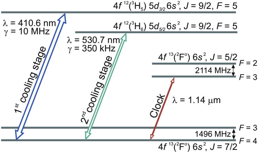
Figure 1: Relevant energy levels of ¹⁶⁹Tm. The strong transition at 410.6 nm is used for the first-stage laser cooling and detecting the ground state populations and the weak transition at 530.7 nm is used for the second-stage cooling. The proposed clock transition $4f^{13}6s^{2}(J=7/2,F=4)\rightarrow 4f^{13}6s^{2}(J=5/2,F=3)$ is at the wavelength of 1.14 um.

In the experimental part (sec. V), we demonstrate direct excitation of the clock transition at 1.14 $\mu$m and measure the lifetime of the upper clock level in a 1D optical lattice formed by 532 nm laser radiation Golovizin et al. (2015). Also, we experimentally evaluate the dynamic polarizability of the Tm ground state at 532 nm by excitation of parametric resonances in the optical dipole trap.

II Polarizabilities

To find the magic wavelength and to estimate the BBR and the van der Waals shifts, one should know the energy shifts $\varDelta E$ of the clock states in an external monochromatic electric field $\vec{E}=\nicefrac{{1}}{{2}}\vec{\mathcal{E}}e^{-i\omega t}+\text{c.c.}$ at the angular frequency $\omega$

$$\varDelta E(\omega)=-\frac{\alpha(\omega)}{4}|\mathcal{E}|^{2}-\frac{\gamma(\omega)}{64}|\mathcal{E}|^{4}+...,$$ (1)

where $\alpha(\omega)$ is the dynamic polarizability and $\gamma(\omega)$ is the hyperpolarizability, both depending on $m$ and the polarization of the field. To our knowledge, there are only a few publications where the polarizability of Tm levels was analyzed. In Rinkleff and Thorn (1994); Rinkleff (1978) the authors measured the static tensor polarizability, while a theoretical calculation of static polarizabilities without accounting for a fine-structure interaction is presented in Chu et al. (2007). In this section we will calculate polarizabilities of the clock states.

To suppress the site-dependent frequency shift from varying light polarization in the lattice, we suggest loading Tm atoms into a 2D optical lattice formed by 4 laser beams with the same linear polarization as shown in Fig. 2. This guarantees that the trapping light polarization is the same for all lattice sites. Further in this paper, we consider only the transition $|J=7/2,F=4,m=0\rangle\rightarrow|J=5/2,F=3,m=0\rangle$ which is free from the frequency shifts induced by the magnetic dipole-dipole interaction (see sec. III). Since both levels have $m=0$, the contribution from the vector polarizability for this transition also vanishes and the total polarizability $\alpha$ can be separated into the scalar $\alpha^{s}$ and the tensor $\alpha^{t}$ parts Lepers et al. (2014) as follows:

$$\begin{split}\alpha_{JFm}(\omega)&=\alpha^{s}_{JF}(\omega)+\alpha^{t}_{JF}(\omega)\frac{3m^{2}-F(F+1)}{F(2F-1)}\,,\\ \alpha^{s}_{JF}(\omega)&=\frac{1}{2F+1}\sum\limits_{m=-F}^{m=F}\alpha_{JFm}(\omega)\,,\\ \alpha^{t}_{JF}(\omega)&=\alpha_{JF,m=F}(\omega)-\alpha^{s}_{JF}(\omega).\end{split}$$ (2)

For consistency with other papers, we will calculate the polarizabilities in atomic units (a.u.); 1 a.u. = $4\pi\epsilon_{0}a_{0}^{3}$ = $1.65\times 10^{-41}$ J/(V/m)², where $a_{0}$ is the Bohr radius and $\epsilon_{0}$ is the vacuum permittivity (for conversion to another units, see Mitroy et al. (2010)).

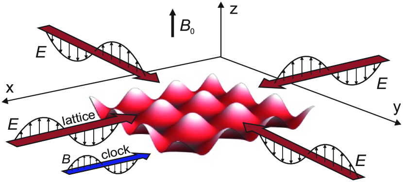
Figure 2: Geometry of a 2D optical lattice. The lattice is formed by 4 horizontal laser beams (lattice, red) with linear vertical polarization. A uniform external magnetic field $B_{0}$ is applied along the vertical axis. An interrogating laser beam (clock, blue) lies in the optical lattice plane (horizontal) to eliminate frequency shifts by the Doppler-effect and photon recoil. The $B$-component of the interrogating light should be vertical to excite the $|m=0\rangle\rightarrow|m=0\rangle$ clock transition (the clock transition is of a magnetic dipole type).

II.1 Discrete spectrum

The contribution of a discrete spectrum is given by Lepers et al. (2014); Angel and Sandars (1968)

$$\alpha_{Fm}(\omega)=\frac{3}{2}\frac{c^{3}\hbar^{4}}{a_{0}^{3}}\sideset{}{{}^{\prime}}{\sum}_{F^{\prime}}\frac{2F_{u}+1}{(E_{F^{\prime}}-E_{F})^{2}}\left(\begin{matrix}F_{u}&1&F_{d}\\ -m&0&m\end{matrix}\right)^{2}\\ \times\frac{A_{F_{u}\to F_{d}}}{(E_{F^{\prime}}-E_{F})^{2}-(\hbar\omega)^{2}},$$ (3)

where $c$ is the speed of light, $\hbar$ is the reduced Planck’s constant, and $E_{F}$ and $E_{F^{\prime}}$ are energies of levels $|F\rangle$ and $|F^{\prime}\rangle$, respectively. The summation is over all levels $F^{\prime}$. For each term, $F_{u}=F^{\prime}$ and $F_{d}=F$ if $E_{F^{\prime}}>E_{F}$ and vice versa. $A_{F_{u}\to F_{d}}$ is a transition probability (spontaneous decay rate) from $|F_{u}\rangle$ to $|F_{d}\rangle$.

Assuming $JI$-coupling between the total electron momentum $J$ and the nuclear spin $I$, the scalar polarizability is independent of $F$ Lepers et al. (2014); Angel and Sandars (1968):

$$\alpha^{s}_{JF}(\omega)=\alpha^{s}_{J}(\omega)=\frac{1}{2J+1}\sum\limits_{m_{J}=-J}^{m_{J}=J}\alpha_{Jm_{J}}(\omega)=\\ \frac{1}{2}\frac{c^{3}}{a_{0}^{3}}\sideset{}{{}^{\prime}}{\sum}_{J^{\prime}}\frac{2J_{u}+1}{2J_{d}+1}\frac{1}{(\omega_{J^{\prime}J})^{2}}\frac{A_{J_{u}\to J_{d}}}{(\omega_{J^{\prime}J})^{2}-\omega^{2}},$$ (4)

where $\omega_{J^{\prime}J}=(E_{J^{\prime}}-E_{J})/\hbar$. The tensor polarizability equals

$$\alpha^{t}_{JF}(\omega)=\alpha^{t}_{J}(\omega)\times(-1)^{I+J+F}\left\{\begin{matrix}F&J&I\\ J&F&2\end{matrix}\right\}\\ \times\sqrt{\frac{F(2F-1)(2F+1)(2J+3)(2J+1)(J+1)}{(2F+3)(F+1)(2J-1)J}},$$ (5)

where

$$\alpha^{t}_{J}(\omega)=\frac{3c^{3}}{a_{0}^{3}}\sideset{}{{}^{\prime}}{\sum}\limits_{J^{\prime}}\frac{2J_{u}+1}{\omega_{J^{\prime}J}^{2}}\frac{A_{J_{u}\rightarrow J_{d}}}{\omega_{J^{\prime}J}^{2}-\omega^{2}}(-1)^{J+J^{\prime}}\\ \times\left\{\begin{matrix}1&1&2\\ J_{d}&J_{d}&J_{u}\end{matrix}\right\}\sqrt{\frac{5J(2J-1)}{6(J+1)(2J+1)(2J+3)}}.$$ (6)

Note that $\alpha^{t}_{\nicefrac{{7}}{{2}},\,4}=\alpha^{t}_{\nicefrac{{7}}{{2}}}$ and $\alpha^{t}_{\nicefrac{{5}}{{2}},\,3}=\alpha^{t}_{\nicefrac{{5}}{{2}}}$.

As an input for calculation of $\alpha$ one should have transition probabilities $A_{J^{\prime}\rightarrow J}$ from the level of interest to all others. Though many transition wavelengths in the spectral range from 250 nm to 807 nm and their probabilities were measured in Wickliffe and Lawler (1997); Anderson et al. (1996) by Fourier-transform spectroscopy and time-resolved laser-induced fluorescence, there is still a number of transitions in the UV, visible, and IR spectral ranges which are essential for calculation and have unknown probabilities. We used the numerical package COWAN Cowan to calculate transition wavelengths and probabilities in the spectral range from 250 nm to 1200 nm (see Appendix A).

The most self-consistent approach for calculation of the differential static polarizability of the clock levels is to use only the numerically calculated wavelengths and probabilities. A slight modification of this approach is used for calculation of the magic wavelengths (sec. II.3).

As expected from general considerations concerning the inner shell transitions, the static scalar polarizabilities for the clock levels are nearly equal. Our calculation shows that they differ by less than $0.1$ a.u. and are equal to 138 a.u. Note, that the calculated static tensor polarizability of $-2.7$ a.u. for the lower $|J=7/2\rangle$ clock level is in good agreement with the known experimental value of $-2.7(2)$ a.u. Rinkleff and Thorn (1994). For the upper $|J=5/2\rangle$ clock level our calculations give $-2.3$ atomic units for the tensor static polarizability.

II.2 Continuous spectrum

To determine a contribution of the continuous spectrum (ignoring hyperfine interaction) to the polarizability we used the formula Veseth and Kelly (1992):

$$\alpha^{s}_{\text{cont}}(\omega)=\frac{c}{2\pi^{2}}\int^{\infty}_{\omega_{I}}\frac{\sigma(\omega^{\prime})d\omega^{\prime}}{(\omega^{\prime}-\omega_{n})^{2}-\omega^{2}},$$ (7)

where $\omega_{I}$ is the photoionization limit and $\sigma(\omega)$ is the photoionization cross section of the energy level. The ionization cross-section was numerically calculated using the package FAC  Gu (2008) and the results are shown in the upper panel of Fig. 3. Using these results, we evaluated the polarizabilities $\alpha^{s}_{\text{cont}}(\omega)$ for the clock levels resulting from transitions to continuous spectrum (Fig. 3, lower panel).

The contributions $\alpha^{s}_{\text{cont}}(\omega)$ are small compared to the contribution from the discrete spectrum and differ only by 2 a.u. for the two fine structure components $|J=7/2\rangle$ and $|J=5/2\rangle$. This means that the transitions to continuum basically do not influence positions of magic wavelengths. We also assume that the corresponding contribution to the tensor polarizability is even smaller and will neglect it in further analysis. Since the discrete spectrum gives the equal static scalar polarizabilities for the clock levels, we expect the continuous spectrum to contribute to polarizabilities of the both levels equally as well. Thus, a rough estimation of the error of calculated contribution of the continuous spectrum to the differential polarizability is about the difference between $\alpha^{s}_{\text{cont}}(0)$ for the clock levels, i.e., 2 a.u. Unfortunately, we do not know of any experimental data on the photoionization cross sections for Tm atoms and therefore can’t rigorously estimate the error.

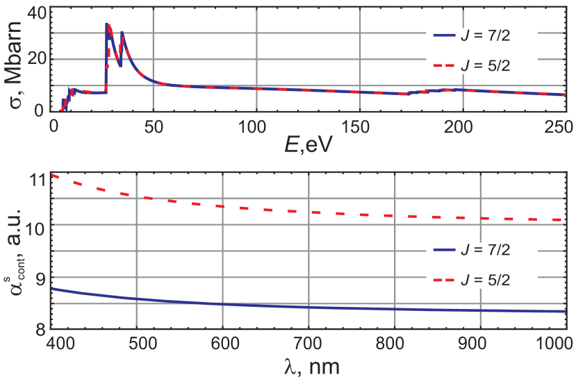
Figure 3: Upper panel: The photoionization cross sections for $|J=7/2\rangle$ (solid blue) and $|J=5/2\rangle$ (dashed red) clock levels. Peaks around 28 and 35 eV correspond to strong resonance enhancement Whitfield et al. (2008). Lower panel: Contribution to the scalar polarizability $\alpha^{s}_{\text{cont}}(\omega)$ from the continuous spectra. The hyperfine interaction is not taken into account.

II.3 Magic wavelength

The magic wavelengths for optical traps providing the vanishing total light shift of the clock transition (1) are widely used in optical clocks Katori et al. (2003). To determine the magic wavelengths one should search for the crossing points of the dynamic polarizabilities for the upper and lower clock levels (neglecting the contribution from the hyperpolarizability in the first approximation). Position of the magic wavelengths strongly depend on energies and probabilities of the resonances in the atom. In general, we can not use only results of our calculations because of insufficient accuracy provided by the COWAN package (see Appendix A).

To solve this problem first we tried a ‘‘combined’’ approach. Calculated transitions were assigned with experimental ones which can be done unambiguously for wavelengths $\lambda>500$ nm. It turns to be impossible for the shorter wavelengths ($\lambda<500$ nm) due to higher density of transitions. Then we combined the calculated spectrum for $\lambda<500$ nm, the available experimental data for $\lambda>500$ nm, and calculated probabilities for known transitions but with not measured probabilities. After detailed study we concluded that it is a questionable approach because the calculated and experimentally measured transition probabilities sometimes differ by an order of magnitude (see Fig. 9, lower panel). This difference impacts the calculated polarizabilities in a wide spectral range impeding reliable prediction of the magic wavelengths.

To our opinion, a more reliable approach bases on maximal use of calculation results: We took the calculated spectrum and substituted the predicted wavelengths with correct ones known from the experiment for all transitions with $\lambda>500$ nm. As for the probabilities, we used the calculated ones except the case when the probability is smaller than $10^{5}$ s^-1. This method give reliable results for the magic wavelengths in the near IR region with low density of strong transitions.

Selected approach predicts the reliable candidate for the magic wavelength at 807 nm with an attractive lattice potential (Fig. 4). Its presence is caused by the weak transition from the $|J=5/2\rangle$ clock level $4f^{13}(^{2}F^{o})6s^{2}(J=5/2)$ with the energy $8771.24\,\text{cm}^{-1}$ to another level $4f^{12}(^{3}F_{4})5d_{3/2}6s^{2}(J=5/2)$, with the energy $21161.4\,\text{cm}^{-1}$ at 807.1 nm  Wickliffe and Lawler (1997). At the same time, there are no allowed transition from the $|J=7/2\rangle$ clock level in the vicinity of 807 nm. Taking into account the uncertainty in the contribution of the continuous spectra to the evaluated differential polarizability of $\pm 1$ a.u., the proposed magic wavelength should be blue-detuned from the transition 807.1 nm by 0.1 nm — 1 nm.

The figure-of-merit for an optical lattice comes from its depth, the off-resonant scattering rate and the magnetic dipole-dipole relaxation rate. The optical lattice depth in kelvin is given by:

$$U\,[\text{K}]=\alpha[\text{a.u.}]\frac{2\pi a_{0}^{3}}{c\,k_{B}}I\,[\text{W/m${}^{2}$}],$$ (8)

where $I$ is the field intensity in lattice anti-nodes given in W/m² and $k_{B}$ is the Boltzmann constant. The spontaneous decay following the off-resonant excitation by the lattice field perturbs the coherence of the clock levels and should be taken into account. The off-resonance scattering rate for the transition $|m=0\rangle\rightarrow|m=0\rangle$ can be estimated as Lepers et al. (2014):

$$\varGamma(\omega)_{0\rightarrow 0}=I\sideset{}{{}^{\prime}}{\sum}\limits_{F^{\prime}}\frac{\omega_{F^{\prime}F}^{2}+\omega^{2}}{\left[\omega_{F^{\prime}F}^{2}-\omega^{2}\right]^{2}}\frac{3\pi c^{2}\,A_{F^{\prime}\rightarrow F}}{\hbar\omega_{F^{\prime}F}^{3}}\\ \times\left(\begin{matrix}F_{u}&1&F_{d}\\ 0&0&0\end{matrix}\right)^{2}(2F_{u}+1)\varGamma_{F_{u}},$$ (9)

where $\varGamma_{F_{u}}$ is the inverse lifetime of $|F_{u}\rangle$ level.

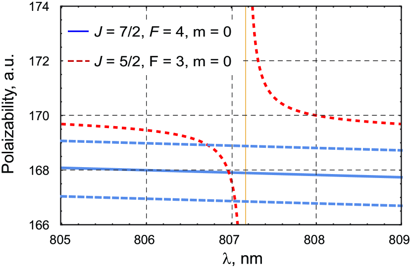
Figure 4: The magic wavelengths for the 1.14 $\mu$m clock transition in Tm atom ($m=0\rightarrow m=0$) around 807 nm calculated for the linear vertical polarization of the trapping light (see Fig. 2). Blue solid curve is the polarizability of the lower $|J=7/2,F=4,m=0\rangle$ clock state, red dashed curve is the polarizability of the upper $|J=5/2,F=3,m=0\rangle$ clock state. The dashed blue lines show the anticipated uncertainty in the calculation of the differential polarizability which may impact the position of the magic wavelength.

The optical lattice at 807 nm can be formed by a Ti:sapphire laser beam. With 0.5 W output power focused in the beam waist of 50 $\mu$m (radius at $1/e^{2}$ intensity level) corresponding to $I=50$ kW/cm² in the retro-reflected configuration, one expects the trap depth of 20 $\mu$K. This is enough to capture Tm atoms from a narrow-line MOT. Even for the smallest expected detuning from the 807.1 nm resonance of 0.1 nm, the off-resonant scattering rate is less than $0.1$ s^-1.

II.4 Hyperpolarizability

The magic wavelength depends not only on the differential polarizability of the clock states, but also on the differential hyperpolarizability (1) and light intensity $I$. The scalar hyperpolarizability $\gamma(\omega)$ is given by Bishop (1994) :

$$\gamma(\omega)=\frac{1}{4}\left(\gamma^{+}(\omega)+\gamma^{-}(\omega)\right),$$ (10)

where

$$\gamma^{+}=\frac{4}{\hbar^{3}}\sideset{}{{}^{\prime}}{\sum}_{m,k,n}(D_{z})_{gm}(D_{z})_{mk}(D_{z})_{kn}(D_{z})_{ng}\\ \times\Bigg{(}\frac{4\omega_{mg}\omega_{ng}}{\omega_{kg}\left(\omega^{2}-\omega_{mg}^{2}\right)\left(\omega^{2}-\omega_{ng}^{2}\right)}\\ +\frac{1}{(\omega_{mg}-\omega)(\omega_{kg}-2\omega)(\omega_{ng}-\omega)}\\ +\frac{1}{(\omega_{mg}+\omega)(\omega_{kg}+2\omega)(\omega_{ng}+\omega)}\Bigg{)}$$ (11)

and

$$\gamma^{-}=\frac{8}{\hbar^{3}}\sideset{}{{}^{\prime}}{\sum}_{m,n}\left|(D_{z})_{mg}\right|^{2}\left|(D_{z})_{ng}\right|^{2}\\ \times\frac{\omega_{mg}\left(\omega^{2}+3\omega_{ng}^{2}\right)}{\left(\omega^{2}-\omega_{mg}^{2}\right)\left(\omega^{2}-\omega_{ng}^{2}\right)^{2}}\,,$$ (12)

where $(D_{z})_{i,j}$ is a matrix element of the $z$-projection of the dipole moment between levels $i$ and $j$.

For calculation of hyperpolarizability we used the transition matrix elements, their signs, and the transition wavelengths obtained by the COWAN package for all transitions except the 807.1 nm one. For this transition, we used the experimentally measured wavelength and probability; the sign of the transition matrix element was taken from the numerical calculations. This exception is done to improve accuracy of the magic wavelength prediction.

The light shifts for the clock levels $|J=7/2\rangle$ and $|J=5/2\rangle$ coming from hyperpolarizability in the optical lattice at $\lambda=807$ nm and $I=50$ kW/cm² is shown in Fig. 5. As follows from the previous section, the magic wavelength is blue detuned from the 807.1 nm resonance by more than 0.1 nm, which makes the hyperpolarizability shift to be less than $0.5$ Hz. Corresponding correction to the magic wavelength is negligible. Still, hyperpolarizability contributes to the clock frequency uncertainty which is discussed later in sec. IV.

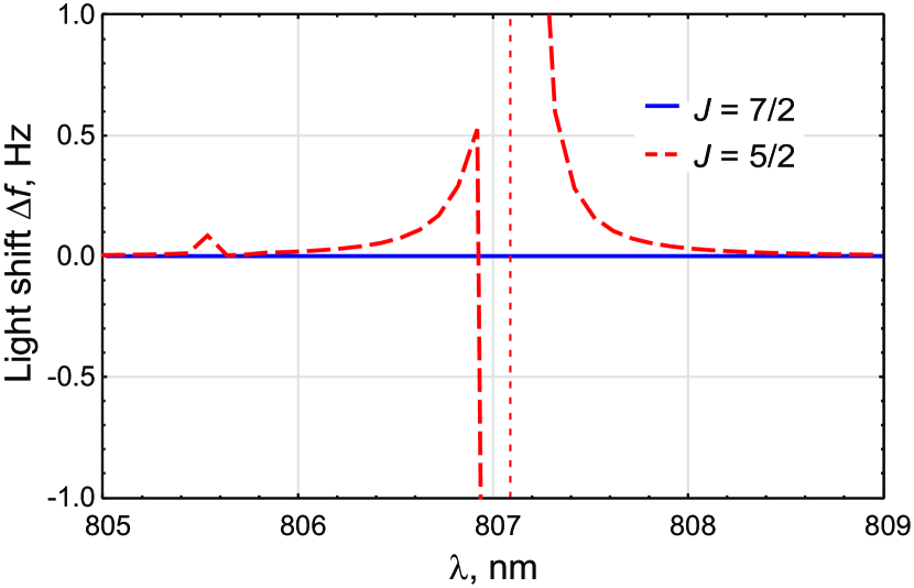
Figure 5: Light shifts of the lower $|J=7/2\rangle$ (blue, solid) and upper $|J=5/2\rangle$ (red, dashed) clock levels caused by the hyperpolarizability. Vertical red line denotes the position of the resonance. Calculations are done for an intensity of $I=50$ kW/cm²; the hyperfine interaction is ignored.

III Magnetic interactions

III.1 Magnetic dipole-dipole interaction

The magnetic moment of the thulium ground state equals $4\mu_{B}$ ($\mu_{B}$ is the Bohr magneton) which causes a magnetic dipole-dipole interaction between atoms. The interaction potential between two atoms is

$$U_{dd}(r)=\mu_{0}(g_{F}\mu_{B})^{2}\frac{\hat{\vec{F_{1}}}\cdot\hat{\vec{F_{2}}}-3(\hat{\vec{F_{1}}}\cdot\hat{\vec{r}})(\hat{\vec{F_{2}}}\cdot\hat{\vec{r}})}{4\pi r^{3}},$$ (13)

where $\vec{F}_{1,2}$ are the total atomic angular momenta, $\mu_{0}$ is the magnetic permeability of vacuum, $\vec{r}$ is the vector pointing from one atom to another and $g_{F}$ is the Landé g-factor of the ground state. For the Tm ground state $g_{F}\approx 1$.

For spatially non-uniform atom distributions over optical lattice sites, the magnetic interaction may lead to inhomogeneous broadening and frequency shifts of the clock transition, both of them being of the same order of magnitude. These shifts correspond to the interaction energy between neighboring atoms. For two Tm atoms loaded in the adjacent sites of optical lattice at 800 nm and prepared in the $|m=4\rangle$ magnetic state, the interaction energy (13) corresponds to the frequency shift of

$$\varDelta f_{dd}\approx\frac{\mu_{0}(m\,\mu_{B})^{2}}{4\pi r^{3}h}\,$$ (14)

which is of the order of 10 Hz. The shift is large and difficult to predict due to randomness of the lattice site occupation. Further, we will analyze only the transition $|m=0\rangle\rightarrow|m=0\rangle$ which is insensitive to this shift.

Magnetic dipole-dipole interactions also limit the interrogation time because of spin relaxation: the atomic ensemble prepared into a pure polarized state will gradually lose its polarization. To evaluate the corresponding relaxation time, we solved the Shrödinger equation with the interaction (13) for 2, 3, 4, and 5 spatially-fixed Tm atoms in ground state ($F_{1}=F_{2}=4$) prepared in the initial $|m=0\rangle\otimes...\otimes|m=0\rangle$ state at the vanishing external magnetic field. The spatial separation of $a=400$ nm corresponds to an 800-nm optical lattice. The relative positions of the atoms are shown in Fig. 6, upper panel. The lower panel of Fig. 6 shows dynamics of the spin state for the central atom, marked blue in the upper panel of Figure.

For 2, 3, and 4 atoms the Shrödinger equation was solved exactly. For 5 atoms the Hilbert space is too large and we restricted our calculation to the subspace $m_{i}=\left\{-2,-1,0,1,2\right\}$ . To estimate validity of this approach we also solved the Shrödinger equation for 2, 3, and 4 atoms in the restricted subspace. The inset in the lower panel of Fig. 6 shows good agreement between approximate and exact solutions for the first 50 ms of the evolution. In the steady-state, it is reasonable to assume that all spin projections are equiprobable. Consequently, average probability to find the central spin in the $|m=0\rangle$ state equals 1/9 for the full Hilbert space and 1/5 for the truncated space. This explains the discrepancy between the exact and approximate solutions at longer times (> 50 ms). The characteristic relaxation time was derived by setting the probability to find the central spin in the initial $|m=0\rangle$ state to 0.7. It equals 20 ms, 13 ms, 11 ms, and 10 ms for 2,3,4, and 5 spins, respectively (Fig. 6).

External magnetic field reduces spin relaxation because some spinflip processes require additional energy. A significant reduction of the spin relaxation is expected if the Zeeman splitting becomes larger than the kinetic energy $E_{K}$ of atoms. At the experimentally achieved temperature of $T\sim 10$ $\mu$K, the kinetic energy equals $E_{K}=k_{B}T\sim 100$ kHz$\times h$. This energy corresponds to a magnetic field of $B\approx E_{K}/(h\mu_{B})$ or approximately 100 mG. We show in the next section that such a bias magnetic field will cause a significant Zeeman shift and cannot not be applied during clock operation. As mentioned in the Introduction, the temperature can be lowered to a few microkelvin which will reduce the threshold magnetic field to a few tens of milligauss which is sufficient for a target clock accuracy.

Assuming that the lattice filling factor is less than unity and taking into account the influence of weak magnetic bias field (10 mG), we conclude that the spin relaxation time should be larger than 10 ms. This sets the bound for the interrogation time of the clock transition and, correspondingly, the Fourier limit of its spectral linewidth of $<10$ Hz. As a result, the spin relaxation should not considerably impact the performance of the proposed optical clock.

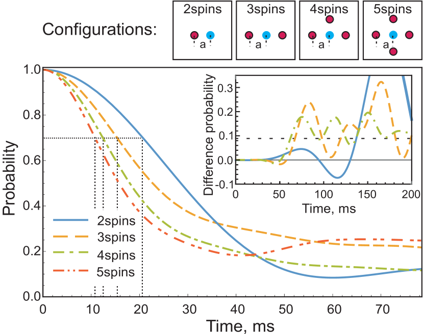
Figure 6: Spin relaxation dynamics. Upper panel: Configurations of atoms used in the simulation, $a=400$ nm is the inter-atomic separation, quantization axes is perpendicular to the plane of the sketch; Main panel: Probability to find the central atom (blue) in the state $|m=0\rangle$ for 2, 3, 4, and 5 atoms in the 2D optical lattice. Note, that the probabilities do not go to zero at longer times because at steady state there is almost uniform distribution among magnetic sublevels. Inset: Difference of the probabilities to find the first atom in the state $|m=0\rangle$ for exact and approximate solutions for 2,3, and 4 atoms. The horizontal dashed line represents the difference of the steady-state probabilities (see the main text).

III.2 Interaction with an external magnetic field

To selectively address the $|m=0\rangle\rightarrow|m=0\rangle$ transition, an external static magnetic field $B$ has to be applied. The Hamiltonian describing hyperfine interaction for the ¹⁶⁹Tm atom ($I=1/2$) in the presence of the external magnetic field $B$ is Giglberger and Penselin (1967):

$$H=hA\hat{\vec{I}}\cdot\hat{\vec{J}}-g_{I}\mu_{N}\hat{\vec{I}}\cdot\hat{\vec{B}}-g_{J}\mu_{B}\hat{\vec{J}}\cdot\hat{\vec{B}},$$ (15)

where $A$ is the hyperfine constant, $g_{I}$ is the nuclear Landé g-factor, $\mu_{N}$ is the nuclear magneton, and $g_{J}$ is the electronic Landé g-factor. The well-known Breit-Rabi formula gives eigenvalues for the special case of $J=1/2$. Making the formal substitution $I\leftrightarrow J$, $g_{I}\leftrightarrow g_{J}$, $\mu_{N}\leftrightarrow\mu_{B}$ in (15) one can use the Breit-Rabi expression for $I=1/2$ Giglberger and Penselin (1967). The frequency shift of the clock transition $|m=0\rangle\rightarrow|m=0\rangle$ is given by

$$\varDelta f_{0\rightarrow 0}=\frac{(g_{5/2}\mu_{B}-g_{I}\mu_{N})^{2}B^{2}}{4h^{2}\varDelta W_{5/2}}\\ -\frac{(g_{7/2}\mu_{B}-g_{I}\mu_{N})^{2}B^{2}}{4h^{2}\varDelta W_{7/2}}=\beta\,B^{2}$$ (16)

and

$$\beta=-257(1)\text{\,Hz}/\text{G}^{2},$$ (17)

where $\varDelta W_{7/2}=1496.550(1)$ MHz, $\varDelta W_{5/2}=2114.946(1)$ MHz are the hyperfine frequency splittings of the $|J=7/2\rangle$ and $|J=5/2\rangle$ clock levels van Leeuwen et al. (1980), and $g_{7/2}=1.141189(3)$ Giglberger and Penselin (1967), $g_{5/2}=0.855(1)$ Blaise and Pierre (1965) are their Landé g-factors, $g_{I}=0.462(3)$ Giglberger and Penselin (1967).

IV Tm clock uncertainty

Here we will discuss the most significant sources of uncertainty for the proposed Tm clock.

IV.1 Black body radiation

The frequency shift of the clock transition due to the AC-Stark shift induced by BBR is given by

$$\varDelta f_{BBR}=\int\limits_{\omega=0}^{\infty}\frac{a_{0}^{3}\omega^{3}}{\pi^{2}c^{2}}\frac{\left(\alpha_{gr}^{s}(\omega)-\alpha_{cl}^{s}(\omega)\right)}{e^{\frac{\hbar\omega}{k_{B}T}-1}}d\omega\\ \approx\varDelta\alpha^{s}_{0}\frac{a_{0}^{3}\pi^{2}k_{B}^{4}}{15c^{3}\hbar^{4}}\,T^{4}=1.17\times 10^{-12}\,\varDelta\alpha^{s}_{0}\text{[a.u.]}\,T^{4}\text{[K]}$$ (18)

where $\varDelta\alpha^{s}_{0}$ is the differential scalar static polarizability of the clock levels in atomic units, $T$ is the temperature in kelvin.

Our calculations (see sec. II) gives $\varDelta\alpha^{s}_{0}=2$ a.u. which results in $\varDelta f_{BBR}=20$ mHz at $T=300$ K. It corresponds to a fractional frequency shift of the clock transition of $8\times 10^{-17}$ which is much less than for the Sr atom and is comparable to Al⁺ clock transition Mitroy et al. (2010). Uncertainty of the ambient temperature of 3 K will introduce a frequency uncertainty of $3\times 10^{-18}$ (0.8 mHz). Since there are no strong transitions from the clock levels in the infrared region the dynamic BBR shift is negligibly small Middelmann et al. (2011).

IV.2 Second order Zeeman shift

According to (16), the frequency shift of the clock transition in the external magnetic field of $B=10$ mG corresponds to $-25.7(1)$ mHz or $10^{-16}$ in fractional units. One can accurately measure the bias field $B$ by monitoring the Zeeman shift of the $|m=-4\rangle\rightarrow|m=-3\rangle$ and $|m=4\rangle\rightarrow|m=3\rangle$ transitions Rosenband et al. (2007). The frequency splitting of these magnetic sensitive transitions in a magnetic field is equal to $\xi=2(4g_{J=7/2,F=4}-3g_{J=5/2,F=3})\mu_{B}/h=6.00(2)$  MHz/G, where $g_{J=7/2,F=4}$ and $g_{J=5/2,3=4}$ are the Landé g-factors of the states $|J=7/2,F=4\rangle$ and $|J=5/2,F=3\rangle$, respectively. Given that the linewidths of both transitions are smaller than $\delta f_{4\rightarrow 3}=100$ Hz (the broadening due to the magnetic interaction (18) is included), the bias magnetic field $B_{0}$ can be measured in situ with the uncertainty of $\varDelta B=\delta f_{4\rightarrow 3}/\xi\leq 0.1$ mG. Since the magnetic field can be stabilized at the same level over the interrogation sequence Rosenband et al. (2008), we take 0.1 mG as an upper limit for the bias magnetic field instability and estimate the quadratic Zeeman shift’s contribution as $2\beta B_{0}\varDelta B_{0}=0.5$ mHz ($2\times 10^{-18}$ in fractional units) after correction.

IV.3 Dynamic light shifts

Fluctuations $\delta I$ of the laser intensity cause shifts and broadening of the clock transition originated from a non-zero differential hyperpolarizability $\varDelta\gamma$:

$$\varDelta f_{I}=-\frac{\delta I}{I}\left(\frac{\varDelta\alpha}{4}I+2\frac{\varDelta\gamma}{64}I^{2}\right)=-\frac{\delta I}{I}\frac{\varDelta\gamma}{64}I^{2}\,,$$ (19)

where we take into account that

$$\frac{\varDelta\alpha}{4}I+\frac{\varDelta\gamma}{64}I^{2}=0$$ (20)

at the magic wavelength. Previously, we estimated that $\varDelta\gamma/64\times I^{2}$ is less than $0.5$ Hz for the given lattice parameters (see sec. II.4). Stabilizing the laser intensity at the level of $10^{-3}$ the uncertainty in the frequency of the clock transition can be reduced to 0.5 mHz or $2\times 10^{-18}$ in fractional units.

IV.4 Van der Waals and quadrupole interactions

The electrostatic van der Waals interaction between two neutral atoms shifts the clock frequency by $-(C_{6}a_{B}^{6}E_{H})/(h\,r^{6}),$ where $C_{6}$ is the van der Waals coefficient in atomic units, $a_{B}$ is the Bohr radius, and $E_{H}$ is the Hartree energy. Following Kotochigova and Petrov (2011), we estimated $C_{6}\sim 6000$ a.u. for $|J=7/2\rangle$ level. For an atomic separation of $r=400$ nm (atoms are placed in the 800-nm optical lattice, less than one atom per site) the van der Waals frequency shift is less than 0.1 mHz which corresponds to $4\times 10^{-19}$ in fractional units.

To estimate the contribution from the quadrupole-quadrupole interaction, we calculated the quadruple moment for the ground state of Tm atom using the COWAN package. The result is $D\sim 0.5\,ea_{B}^{2}$ ($e$ is the elementary charge). The corresponding frequency shift is $D^{2}/(4\pi\epsilon_{0}r^{5}h)<0.1$ mHz.

IV.5 Line pulling and geometrical effects

In an external bias magnetic field of $B=10$ mG, the $|J=7/2,F=4\rangle\rightarrow|J=5/2,F=3\rangle$ transition will be split into magnetic components. The line pulling effect de Marchi et al. (1984) can perturb the magnetic-insensitive clock $|m=0\rangle\rightarrow|m=0\rangle$ transition. Imperfect co-alignment of the magnetic field $B$ and the polarization of the interrogating laser beam (Fig. 2) leads to excitation of $|m=0\rangle\rightarrow|m=\pm 1\rangle$ transitions and also can cause the line pulling effect.

In both cases, the separation from the clock transition to the nearest transition is not less than $10^{3}\gamma\approx$ 20 kHz, where $\gamma=20$ Hz is the upper bound for the expected transition linewidth. The corresponding incoherent line pulling is negligible ($<10^{-8}$ Hz) and does not impact the clock performance. For reading the clock transition, absorption spectroscopy is typically used and we do not expect a contribution from the coherent line pulling  Beyer et al. (2015).

Another systematic effect related to the geometry can come from misalignment of the lattice light polarization and the bias magnetic field (see Fig. 2). The shift results from the differential tensor polarizability of the clock levels $\varDelta\alpha^{t}$ and scales as the square of the misalignment angle Nicholson et al. (2015). It was shown that the corresponding relative frequency shift can be reduced to less than $2\times 10^{-18}$ by proper alignment Nicholson et al. (2015).

IV.6 Uncertainty budget

Table 1: Uncertainty budget for a Tm optical clock operating at the 1.14 $\mu$m magnetic dipole transition. Atoms are trapped in the optical lattice at the magic wavelength close to 807 nm with the light intensity of 50 kW/cm².

Contribution	Frequency shift, mHz	Uncertainty after correc- tion, mHz	Uncertainty in fractional units, $10^{-18}$
BBR ($T=300\pm 3$ K)	20	0.8	3
Zeeman shift ($B=10.0\pm 0.1$ mG)	$-26$	0.5	2
Light shift due to hyperpolarizability ($\delta I/I=10^{-3}$)	0	0.5	2
Light shift due to tensor polarizability	0.5	0.5	2
van der Waals and quadrupole interaction	0.1	0.1	0.4
Total	$-6$	1.2	$<5$

The list of dominant frequency shifts and corresponding uncertainties is presented in Table 1. The major line shifts are the BBR shift and the second-order Zeeman shift. All of these can be well characterized and corrected to a high degree using moderate assumptions and established experimental techniques. Light shift can also be controlled at low $10^{-18}$ level by intensity stabilization of the light field. As a result, the systematic frequency uncertainty of the proposed Tm optical clock at $1.14$ $\mu$m can be reduced to $5\times 10^{-18}$ in fractional units.

V Experiment

The experimental section describes our measurement of the $|J=5/2\rangle$ clock level lifetime in a dilute cloud of cold Tm atoms. Formerly, the decay from this level was studied in Tm atoms implanted in solid and liquid ⁴He Ishikawa et al. (1997). Strong shielding of inner shells and the high symmetry of the perturbing field of the He matrix give the impressive result of 75(3) ms for the lifetime of the $|J=5/2\rangle$ clock level. Note that the level was populated by a cascade decay from highly excited levels.

In contrast to Ishikawa et al. (1997), we directly excite the $|J=7/2,F=4\rangle\rightarrow|J=5/2,F=3\rangle$ transition by spectrally narrow laser radiation at 1.14 $\mu$m in an ensemble of Tm atoms trapped in a 1D optical lattice and measure the lifetime of the $|J=5/2\rangle$ clock level monitoring its decay to the ground $|J=7/2,F=4\rangle$ state. Besides that, we evaluated dynamic polarizability of Tm atoms at 532 nm by exciting parametric resonances in an optical lattice.

V.1 Lifetime of the $|J=5/2\rangle$ clock level

The lifetime of $|J=5/2\rangle$ clock level is measured by excitation of the magnetic dipole transition at 1.14 $\mu$m in a 1D optical lattice. About $10^{6}$ thulium atoms are laser cooled down to 20 $\mu$K in a narrow-line MOT operating at 530.7 nm Sukachev et al. (2014) and then are recaptured by the 1D optical lattice. The lattice is formed by a retro-reflected focused 532 nm cw laser beam (waist radius is 50 $\mu$m, laser power is 3 W) and superimposed with the atomic cloud. The trap depth is calculated to be 400 $\mu$K for the ground $|J=7/2,F=4\rangle$ state which provides a recapture efficiency of 40% Sukachev et al. (2014).

After recapture (pulse 1 in Fig. 7), we switch the MOT off and wait for 20 ms to let uncaptured atoms escape. Then, a resonant 1.14 $\mu$m laser pulse of 30 ms (pulse 2) is applied to excite atoms to the $|J=5/2,F=3\rangle$ level Golovizin et al. (2015). The laser is actively stabilized to a high-finesse ULE cavity Alnis et al. (2008) which narrows the laser spectral linewidth down to $\sim 10$ Hz. After the interrogation pulse, a resonant 410.6 nm laser pulse of 1 ms (pulse 3) is applied to remove atoms from the $|J=7/2\rangle$ ground state (Fig. 1). Atoms exited to the $|J=5/2,F=3\rangle$ decay back to the $|J=7/2,F=4\rangle$ ground state, which population is monitored by a fluorescence signal induced by a delayed 410.6 nm probe pulse (pulse 4).

The increase of the population of the $|J=7/2,F=4\rangle$ ground state is described by the exponential function

$$N(t)=N_{0}(1-\exp(-{t}/{\tau})),$$ (21)

where $\tau$ is the lifetime of the the excited $|J=5/2,F=3\rangle$ state and $N_{0}$ is the initial number of atoms in this state. By fitting the experimental data presented in Fig. 7, we measure $\tau=112(4)$ ms. It is the lower bound for the $|J=5/2\rangle$ level natural lifetime since the measured lifetime can be reduced by additional weak losses from the $|J=5/2\rangle$ level in the optical lattice. These losses may be related to optical or magnetic Feshbach resonances Chin et al. (2010).

Thus, the natural linewidth of the clock transition $|J=7/2\rangle\rightarrow|J=5/2\rangle$ is expected to be not broader than 1.4 Hz which is consistent with the previous measurement in ⁴He matrix Ishikawa et al. (1997) and the theoretical prediction of 1.14 Hz Kolachevsky et al. (2007). The natural linewidth of the transition does not limit the performance of the proposed optical clock (see sec. IV), because for most routinely operating optical clocks the Fourier-limited spectral linewidth of the clock transition is on the order of 10 Hz.

In the current experimental arrangement we observed the spectral linewidth of the $|J=7/2,F=4\rangle\rightarrow|J=5/2,F=3\rangle$ transition of 1 MHz at the low power limit Vishnyakova, G A, Golovizin, A A Kalganova et al. (2016). It is due to Zeeman splitting in the un-compensated laboratory field ($\sim 0.5$ MHz) and inhomogeneous power broadening caused by different dynamic polarizabilities of the $|J=7/2,F=4\rangle$ and $|J=5/2,F=3\rangle$ levels at 532 nm ($\sim 0.4$ MHz).

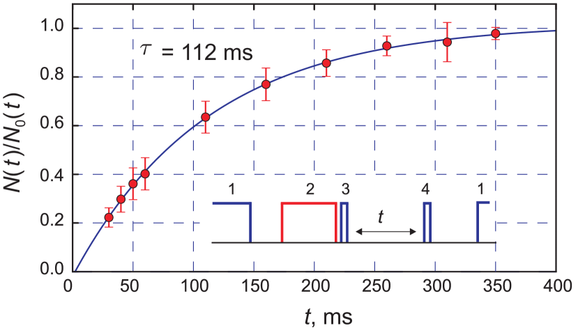
Figure 7: Measurement of the lifetime of the $|J=5/2\rangle$ level. Red dots are the normalized number of atoms decayed to the ground $|J=7/2,F=4\rangle$ level. The solid curve is a fit by (21). The inset shows the pulse sequence described in the text.

V.2 Parametric resonances

The dynamic polarizability of the $|J=7/2\rangle$ ground state at the lattice wavelength can be evaluated by the excitation of parametric resonances in the lattice and by monitoring the corresponding losses Friebel et al. (1998). This method is very sensitive to the laser beam parameters (waist size, astigmatism) and does not allow accurate comparison to our calculations. Still, it gives the proper order of magnitude for the polarizability and provides unambiguous proof that Tm atoms are localized in the 1D optical lattice.

At low temperatures, atomic motion in the optical lattice becomes quantized and the corresponding axial $f_{a}$ and radial $f_{r}$ oscillation frequencies at the center of the lattice are given by

$$\begin{split}f_{a}=&\frac{4}{w_{0}\lambda}\sqrt{\frac{2a_{0}^{3}\alpha^{s}P}{cm_{0}}}\,,\\ f_{r}=&\frac{4}{\pi w_{0}^{2}}\sqrt{\frac{a_{0}^{3}\alpha^{s}P}{cm_{0}}}\,,\end{split}$$ (22)

where $P=4$ W is the optical power of the laser beam forming the 1D lattice, $m_{0}$ is the Tm atomic mass, $w_{0}$ is the beam waist radius (at $1/e^{2}$ intensity level), $\lambda=532$ nm is the lattice wavelength, and $\alpha^{s}$ is the scalar polarizability at $\lambda=532$ nm of the $|J=7/2,F=4\rangle$ level in atomic units. According to Landau and Lifshits (1976), harmonic modulation of the trap depth at frequencies $2f/n$ (here $f$ is one of the eigenfrequencies (22) and $n$ is an integer) will cause parametric excitation of the resonances and corresponding trap losses.

To excite parametric resonances in the 532 nm optical lattice, we harmonically modulated the laser power and, correspondingly, the trap depth by an acousto-optical modulator (AOM) at the level of 10%. The number of atoms remaining in the optical lattice after 100 ms of parametric excitation was monitored by resonance fluorescence at 410.6 nm. The corresponding spectrum is shown in Fig. 8. The low frequency parametric resonances at $400(40)$ Hz and $900(150)$ Hz correspond to the radial oscillations at $f_{r}$ and $2f_{r}$ frequencies. The high frequency resonances at $230(40)$ kHz and $420(50)$ kHz are related to axial oscillations at $f_{a}$ and $2f_{a}$ in the tight potential wells of the lattice. Higher order parametric resonances are much weaker and broader Landau and Lifshits (1976) and were not observed.

The scalar polarizability can be deduced from (22) by excluding $w_{0}$:

$$\alpha^{s}=\frac{f_{a}^{4}\lambda^{4}cm_{0}}{64f_{r}^{2}a_{0}^{3}\pi^{2}P}\,.$$ (23)

From the measured frequencies we estimate this value to be $360^{+300}_{-200}$ a.u. which agrees with the calculated polarizability of 600 a.u. within error bars. The main sources of uncertainty are astigmatism in the lattice beams, axial and radial misalignment of the waist positions of the lattice beams, and error in our determination of the parametric resonance frequency.

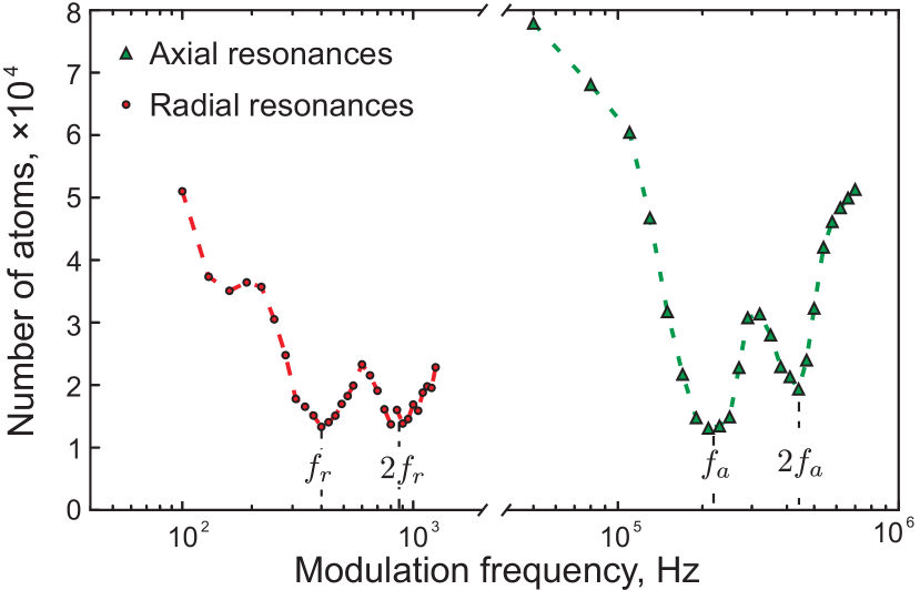
Figure 8: Excitation of the parametric resonances in the 532 nm 1D optical lattice. Green triangles are axial resonances, red circles are radial ones; dashed curves are guides to the eyes.

In conclusion, the experimental results for the scalar dynamic polarizability $\alpha^{s}$ at 532  nm in the optical lattice and in the dipole trap are consistent with the calculated value of 600 a.u. Although the experiment does not allow to test the accuracy of our calculations, it unambiguously proves trapping Tm atoms in the optical lattice at 532 nm.

VI Summary

We considered the possibility to use the inner-shell transition $[\text{Xe}]4f^{13}6s^{2}(J=7/2,\,F=4,\,m=0)\rightarrow[\text{Xe}]4f^{13}6s^{2}(J=5/2,\,F=3,\,m=0)$ in the Tm atom at $\lambda=1.14\,\mu$m as a candidate for an optical lattice clock. The transition wavelengths and probabilities for two clock levels $|J=7/2\rangle$ and $|J=5/2\rangle$ in the spectral range 250 nm — 1200 nm are calculated using the COWAN package which allows deducing of the differential dynamic polarizability and suggests that the magic wavelength is at around 807 nm with an attractive optical potential. Our calculations show a reasonable correspondence with existing experimental data and significantly extend it to the UV and IR spectral ranges.

The suggested clock transition demonstrates a low sensitivity to the BBR shift which provides a clock frequency instability at the low $10^{-18}$ level competing with the best known optical clocks. We also evaluated other feasible contributions to clock performance (magnetic interactions, light shifts, van der Waals, and quadrupole shifts) which, after reasonable assumptions, can be lowered to the $10^{-18}$ level. Together with the relative simplicity of laser cooling and trapping Tm atoms, our results demonstrate that Tm is a promising candidate for optical clock applications. One of the disadvantages is the relatively low carrier frequency of only $2.6\times 10^{14}$ Hz which requires longer integration time to reach the same instability as Sr and Yb lattice clocks.

Our experiments with direct excitation of the clock transition by spectrally narrow laser radiation at $\lambda=1.14\,\mu$m set a lower limit for the upper clock level lifetime of 112 ms which corresponds to the natural linewidth of $<1.4$ Hz. Experiments were done in a 1D optical lattice at 532 nm. Modulating the trap depth and analyzing the corresponding parametric resonances frequencies, we deduced the scalar polarizability of the Tm ground state at 532 nm which shows reasonable agreement with our calculations.

To experimentally study the magic wavelength and analyze systematic shifts, we plan to change the trapping wavelength to 806 nm — 807 nm using a tunable Ti:sapphire laser. This will also simplify our study of Feshbach resonances and may open a way to study and control dipole-dipole interactions using narrow band excitation of the clock transition at 1.14 nm.

Appendix A Transition probabilities

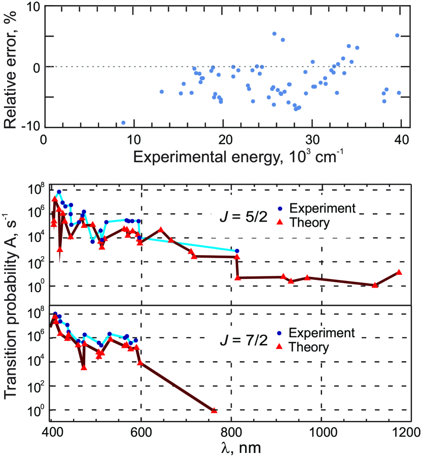
Figure 9: Comparison between the calculated and measured data. Only levels which were identified with the experimentally measured ones are shown. Upper panel: Relative error of calculated energy levels. Lower panel: Calculated (red triangles) and measured (blue circles) transition probabilities from the upper $|J=5/2\rangle$ and the lower $|J=7/2\rangle$ clock levels. Solid curves are guides for the eyes only.

Table 2: Calculated (experimentally unmeasured) transition probabilities from the $|J=7/2\rangle$ and $|J=5/2\rangle$ clock levels. $E$ and $J$ are experimentally measured energies and electronic angular momenta of the upper levels of the transitions, respectively.

$E$, $10^{3}$ cm-1	J	$\lambda$, nm	$A$ c-1
$|J=7/2\rangle$ level
$13\,119.6$	$\nicefrac{{9}}{{2}}$	$762.22$	$3.2$
$16\,742.2$	$\nicefrac{{7}}{{2}}$	$597.29$	$1.9\times 10^{5}$
$19\,748.5$	$\nicefrac{{9}}{{2}}$	$506.37$	$1.2\times 10^{6}$
$|J=5/2\rangle$ level
$16\,742.2$	$\nicefrac{{7}}{{2}}$	$1254.55$	$14.1$
$16\,957.0$	$\nicefrac{{7}}{{2}}$	$1221.63$	$1.2$
$17\,343.4$	$\nicefrac{{7}}{{2}}$	$1166.57$	$171.2$
$17\,752.6$	$\nicefrac{{5}}{{2}}$	$1113.41$	$27.5$
$19\,132.2$	$\nicefrac{{3}}{{2}}$	$965.16$	$150$
$19\,548.8$	$\nicefrac{{5}}{{2}}$	$927.85$	$100$
$19\,753.8$	$\nicefrac{{7}}{{2}}$	$910.53$	$209$
$21\,120.8$	$\nicefrac{{7}}{{2}}$	$809.74$	$640$
$22\,791.2$	$\nicefrac{{7}}{{2}}$	$713.27$	$27\,400$
$22\,929.7$	$\nicefrac{{5}}{{2}}$	$706.29$	$58\,900$
$23\,873.2$	$\nicefrac{{7}}{{2}}$	$662.17$	$1\times 10^{6}$
$23\,882.4$	$\nicefrac{{3}}{{2}}$	$661.76$	$2.13\times 10^{6}$
$24\,418.4$	$\nicefrac{{5}}{{2}}$	$639.11$	$1.79\times 10^{7}$

Calculation of dynamic polarizabilities eq. (3-5) requires knowledge of electrical dipole transition rates from the lower $|J=7/2\rangle$ and the upper $|J=5/2\rangle$ clock levels in Tm. A number of transitions rates were experimentally measured and the results are summarized in Wickliffe and Lawler (1997). We completed this list by calculation of energy levels in the range up to 40000 cm^-1 and corresponding transition-dipole matrix elements using the COWAN package Cowan taking into account the low lying odd ($4f^{13}6s^{2}$, $4f^{13}5d^{1}6s^{1}$, $4f^{12}6s^{2}6p^{1}$, $4f^{13}6p^{2}$, $4f^{13}5d^{2}$) and even ($4f^{12}5d^{1}6s^{2}$, $4f^{13}6s^{1}6p^{1}$) configurations.

As follows from the upper panel of Fig. 9, the accuracy of the calculated level energies is better than 20%. Together with the known leading configuration percentage it is sufficient to identify the low laying levels with the energies $E<20000$ cm^-1 ($\lambda>500$ nm) and compare them with the experimentally measured ones Martin et al. (1978). Table 2 shows calculated probabilities of the transitions with experimentally unknown probabilities from the clock levels $[\text{Xe}]4f^{13}6s^{2}(J=7/2)$ and $[\text{Xe}]4f^{13}6s^{2}(J=5/2)$. The lower panel of Fig. 9 shows comparison between the experimentally measured and calculated transition probabilities in the range from 500 nm to 1200 nm where level identification can be done unambiguously. Taking into account difficulties with simulation of the hollow-shell atomic potentials Lepers et al. (2014), the discrepancy between the calculated and the experimental data seems to be reasonable.

As mentioned in the main text, the most self-consistent approach for deriving differential polarizability of the clock levels is to use the calculated data for the transition probabilities, otherwise we meet difficulties with level identification in the wavelength range $\lambda<500$ nm and with matching the calculated and the experimental data. In turn, transitions to the highly excited Rydberg states ($\lambda<250$ nm) become extremely dense and COWAN package cannot be used. To calculate their contribution one typically uses semi-analytical approach Chernov et al. (2005). In our case, strong similarity of spectra starting from two inner-shell fine structure sublevels – clock levels ($|J=7/2\rangle$ and $|J=5/2\rangle$) – results in very small differential polarizability of 0.1 a.u. if one takes into account all transitions in the spectral range 250 nm — 1200 nm. Transitions to the Rydberg states may slightly influence the absolute values of the polarizability of the clock states (at the level of a few a.u.), but we do not expect significant contribution to the differential polarizability $\varDelta\alpha$.

References

- E V Zharikov, V I Zhekov, L A Kulevskii, T M Murina et al. (1975) V. V. E V Zharikov, V I Zhekov, L A Kulevskii, T M Murina, A. M. Osiko, A. D. Prokhorov, Savel’ev, V V Smirnov, B P Starikov, and M I Timoshechkin, Sov J Quantum Electron 4, 1039 (1975).
- Barnes et al. (1993) N. P. Barnes, E. D. Filer, F. L. Naranjo, W. J. Rodriguez, and M. R. Kokta, Optics Letters 18, 708 (1993).
- Böttger et al. (2001) T. Böttger, G. J. Pryde, N. M. Strickland, P. B. Sellin, and R. L. Cone, Optics and Photonics News 12, 23 (2001).
- Aleksandrov et al. (1983) E. Aleksandrov, V. Kotylev, V. Kulyasov, and K. Vasilevskii, Opt. Spektrosk. 54, 3 (1983).
- Wilpers et al. (2002) G. Wilpers, T. Binnewies, C. Degenhardt, U. Sterr, J. Helmcke, and F. Riehle, Physical Review Letters 89, 230801 (2002).
- Ido et al. (2005) T. Ido, T. H. Loftus, M. M. Boyd, A. D. Ludlow, K. W. Holman, and J. Ye, Physical Review Letters 94, 153001 (2005).
- Hancox et al. (2004) C. I. Hancox, S. C. Doret, M. T. Hummon, L. Luo, and J. M. Doyle, Nature 431, 281 (2004).
- Connolly et al. (2010) C. B. Connolly, Y. S. Au, S. C. Doret, W. Ketterle, and J. M. Doyle, Physical Review A 81, 010702 (2010).
- Katori et al. (2003) H. Katori, M. Takamoto, V. G. Pal’chikov, and V. D. Ovsiannikov, Physical Review Letters 91, 173005 (2003).
- Takamoto and Katori (2003) M. Takamoto and H. Katori, Physical review letters 91, 223001 (2003).
- Ludlow et al. (2015) A. D. Ludlow, M. M. Boyd, J. Ye, E. Peik, and P. O. Schmidt, Reviews of Modern Physics 87, 637 (2015).
- Bloom et al. (2014) B. J. Bloom, T. L. Nicholson, J. R. Williams, S. L. Campbell, M. Bishof, X. Zhang, W. Zhang, S. L. Bromley, and J. Ye, Nature 506, 71 (2014).
- Hinkley et al. (2013) N. Hinkley, J. A. Sherman, N. B. Phillips, M. Schioppo, N. D. Lemke, K. Beloy, M. Pizzocaro, C. W. Oates, and A. D. Ludlow, Science (New York, N.Y.) 341, 1215 (2013).
- Beloy et al. (2014) K. Beloy, N. Hinkley, N. B. Phillips, J. A. Sherman, M. Schioppo, J. Lehman, A. Feldman, L. M. Hanssen, C. W. Oates, and A. D. Ludlow, Physical Review Letters 113, 260801 (2014).
- Safronova et al. (2013) M. S. Safronova, S. G. Porsev, U. I. Safronova, M. G. Kozlov, and C. W. Clark, Physical Review A 87, 012509 (2013).
- Ushijima et al. (2015) I. Ushijima, M. Takamoto, M. Das, T. Ohkubo, and H. Katori, Nature Photonics 9, 185 (2015).
- Kulosa et al. (2015) A. P. Kulosa, D. Fim, K. H. Zipfel, S. Rühmann, S. Sauer, N. Jha, K. Gibble, W. Ertmer, E. M. Rasel, M. S. Safronova, U. I. Safronova, and S. G. Porsev, Physical Review Letters 115, 240801 (2015), arXiv:1508.01118 .
- McFerran et al. (2014) J. J. McFerran, L. Yi, S. Mejri, W. Zhang, S. Di Manno, M. Abgrall, J. Guéna, Y. Le Coq, and S. Bize, Physical Review A 89, 043432 (2014).
- Aikawa et al. (2012) K. Aikawa, A. Frisch, M. Mark, S. Baier, A. Rietzler, R. Grimm, and F. Ferlaino, Physical Review Letters 108, 210401 (2012).
- Lu et al. (2011) M. Lu, N. Q. Burdick, S. H. Youn, and B. L. Lev, Phys. Rev. Lett. 107, 190401 (2011).
- Sukachev et al. (2010) D. Sukachev, A. Sokolov, K. Chebakov, A. Akimov, S. Kanorsky, N. Kolachevsky, and V. Sorokin, Physical Review A 82 (2010).
- Sukachev et al. (2014) D. D. Sukachev, E. S. Kalganova, A. V. Sokolov, S. A. Fedorov, G. A. Vishnyakova, A. V. Akimov, N. N. Kolachevsky, and V. N. Sorokin, Quantum Electronics 44, 515 (2014).
- Alnis et al. (2008) J. Alnis, A. Matveev, N. Kolachevsky, T. Udem, and T. W. Hänsch, Physical Review A 77, 053809 (2008).
- Kessler et al. (2012) T. Kessler, C. Hagemann, C. Grebing, T. Legero, U. Sterr, F. Riehle, M. J. Martin, L. Chen, and J. Ye, Nature Photonics 6, 687 (2012).
- Vishnyakova, G A, Golovizin, A A Kalganova et al. (2016) E. K. Vishnyakova, G A, Golovizin, A A Kalganova, V. N. Sorokin, and N. N. Sukachev, D D Tregubov, D O Khabarova, K Yu Kolachevsky, Physics-Uspekhi 59, 168 (2016).
- Frisch (2014) A. Frisch, Dipolar Quantum Gases of Erbium, Ph.D. thesis, University of Inssbruck (2014).
- Ketterle and Van Druten (1996) W. Ketterle and N. J. Van Druten, in Atomic, Molecular, and Optical Physics Volume 37, edited by B. B. Walther and Herbert (Academic Press, 1996) pp. 181–236.
- Dalibard (1998) J. Dalibard, Proceedings of the International School of Physics ’Enrico Fermi’, Course CXL: ’Bose- Einstein condensation in gases’, edited by M. Inguscio, S. Stringari, and C. Wieman (IOS press, Varenna, 1998) pp. 321–350.
- Gribakin and Flambaum (1993) G. F. Gribakin and V. V. Flambaum, Physical Review A 48, 546 (1993).
- Golovizin et al. (2015) A. A. Golovizin, E. S. Kalganova, D. D. Sukachev, G. A. Vishnyakova, I. A. Semerikov, V. V. Soshenko, D. O. Tregubov, A. V. Akimov, N. N. Kolachevsky, K. Y. Khabarova, and V. N. Sorokin, Quantum Electronics 45, 482 (2015).
- Rinkleff and Thorn (1994) R.-H. Rinkleff and F. Thorn, Zeitschrift für Physik D Atoms, Molecules and Clusters 32, 173 (1994).
- Rinkleff (1978) R.-H. Rinkleff, Zeitschrift für Physik A Atoms and Nuclei 288, 233 (1978).
- Chu et al. (2007) X. Chu, A. Dalgarno, and G. C. Groenenboom, Phys. Rev. A 75, 032723 (2007).
- Lepers et al. (2014) M. Lepers, J.-F. Wyart, and O. Dulieu, Physical Review A 89, 022505 (2014).
- Mitroy et al. (2010) J. Mitroy, M. S. Safronova, and C. W. Clark, Journal of Physics B: Atomic, Molecular and Optical Physics 43, 202001 (2010).
- Angel and Sandars (1968) J. R. P. Angel and P. G. H. Sandars, Proceedings of the Royal Society A: Mathematical, Physical and Engineering Sciences 305, 125 (1968).
- Wickliffe and Lawler (1997) M. E. Wickliffe and J. E. Lawler, Journal of the Optical Society of America B 14, 737 (1997).
- Anderson et al. (1996) H. M. Anderson, E. A. D. Hartog, and J. E. Lawler, Journal of the Optical Society of America B 13, 2382 (1996).
- (39) R. Cowan, The Theory of Atomic Structure and Spectra (University of California Press, Berkeley, CA, 1981), and Cowan programs RCN, RCN2, and RCG.
- Veseth and Kelly (1992) L. Veseth and H. P. Kelly, Physical Review A 45, 4621 (1992).
- Gu (2008) M. F. Gu, Canadian Journal of Physics 86, 675 (2008).
- Whitfield et al. (2008) S. B. Whitfield, K. Caspary, R. Wehlitz, and M. Martins, Journal of Physics B 41, 015001 (2008).
- Bishop (1994) D. M. Bishop, The Journal of Chemical Physics 100, 6535 (1994).
- Giglberger and Penselin (1967) D. Giglberger and S. Penselin, Zeitschrift fuer Physik 199, 244 (1967).
- van Leeuwen et al. (1980) K. van Leeuwen, E. Eliel, and W. Hogervorst, Physics Letters A 78, 54 (1980).
- Blaise and Pierre (1965) J. Blaise and C. Pierre, Comptes rendus de l’Académie des sciences. 260, 4693 (1965).
- Middelmann et al. (2011) T. Middelmann, C. Lisdat, S. Falke, J. S. R. Winfred, F. Riehle, and U. Sterr, IEEE Transactions on Instrumentation and Measurement 60, 2550 (2011).
- Rosenband et al. (2007) T. Rosenband, P. Schmidt, D. Hume, W. Itano, T. Fortier, J. Stalnaker, K. Kim, S. Diddams, J. Koelemeij, J. Bergquist, and D. Wineland, Physical Review Letters 98, 220801 (2007).
- Rosenband et al. (2008) T. Rosenband, D. B. Hume, P. O. Schmidt, C. W. Chou, A. Brusch, L. Lorini, W. H. Oskay, R. E. Drullinger, T. M. Fortier, J. E. Stalnaker, S. A. Diddams, W. C. Swann, N. R. Newbury, W. M. Itano, D. J. Wineland, and J. C. Bergquist, Science 319, 1808 (2008).
- Kotochigova and Petrov (2011) S. Kotochigova and A. Petrov, Physical chemistry chemical physics : PCCP 13, 19165 (2011).
- de Marchi et al. (1984) A. de Marchi, G. D. Rovera, and A. Premoli, Metrologia 20, 37 (1984).
- Beyer et al. (2015) A. Beyer, L. Maisenbacher, K. Khabarova, A. Matveev, R. Pohl, T. Udem, T. W. Hänsch, and N. Kolachevsky, Physica Scripta T165, 014030 (2015).
- Nicholson et al. (2015) T. L. Nicholson, S. L. Campbell, R. B. Hutson, G. E. Marti, B. J. Bloom, R. L. McNally, W. Zhang, M. D. Barrett, M. S. Safronova, G. F. Strouse, W. L. Tew, and J. Ye, Nature communications 6, 6896 (2015).
- Ishikawa et al. (1997) K. Ishikawa, A. Hatakeyama, K. Gosyono-o, S. Wada, Y. Takahashi, and T. Yabuzaki, Physical Review B 56, 780 (1997).
- Chin et al. (2010) C. Chin, R. Grimm, P. Julienne, and E. Tiesinga, Reviews of Modern Physics 82, 1225 (2010).
- Kolachevsky et al. (2007) N. Kolachevsky, A. Akimov, I. Tolstikhina, K. Chebakov, A. Sokolov, P. Rodionov, S. Kanorski, and V. Sorokin, Applied Physics B 89, 589 (2007).
- Friebel et al. (1998) S. Friebel, C. D Andrea, J. Walz, M. Weitz, and T. W. Haensch, Physical Review A 57, R20 (1998).
- Landau and Lifshits (1976) L. D. Landau and E. M. Lifshits, Mechnics, 3rd ed. (Pergamon press, 1976).
- Martin et al. (1978) W. C. Martin, R. Zalubas, and L. Hagan, Atomic Energy Levels: The Rare-Earth Elements (Nat. Bur. Stand., U.S., 1978).
- Chernov et al. (2005) V. E. Chernov, D. L. Dorofeev, I. Y. Kretinin, and B. A. Zon, Journal of Physics B 38, 2289 (2005).