From Pseudo-bosons to Pseudo-Hermiticity via multiple generalized Bogoliubov transformations

Abstract:

We consider the special type of pseudo-bosonic systems that can be mapped to standard bosons by means of generalized Bogoliubov transformation and demonstrate that a pseudo-Hermitian systems can be obtained from them by means of a second subsequent Bogoliubov transformation. We employ these operators in a simple model and study three different types of scenarios for the constraints on the model parameters giving rise to a Hermitian system, a pseudo-Hermitian system in which the second the Bogoliubov transformations is equivalent to the associated Dyson map and one in which we obtain D-quasi bases.

1 Introduction

The basic principles for a consistent time-independent quantum mechanical treatment of quasi/pseudo-Hermitian and/or $\mathcal{PT}$-symmetric Hamiltonians are well understood theoretically and by now widely accepted, see e.g. [1, 2, 3, 4] for an overview. In addition, many experiments have been carried out to confirm the key findings of this approach and to make further predictions, see e.g. [5, 6, 7].

A central element in such considerations is the construction of the so-called Dyson map [8] that adjointly transforms a non-Hermitian Hamiltonian to a Hermitian isospectral counterpart. Subsequently this map can be used to manufacture a new metric operator for the physical Hilbert space. This programme is conceptually straightforward, but it remains a technical challenge even for simple examples [9, 10]. Nonetheless, it has been carried out successfully for many concrete models [11, 12, 13, 14, 15]. Alternatively, one may also attempt to transform a model’s more basic constituents, such as Lie algebraic [15] or bosonic [16, 15] building blocks by different types of transformations. By viewing the adjoint map as a generalized Bogoliubov transformation we pursue here a combined approach to achieve this goal. In [17] we found that when the constraint on the target Hamiltonian to be Hermitian is relaxed, the generalized Bogoliubov transformations still lead to systems with $\mathcal{D}$-pseudo-bosons, see e.g. [18] for an overview, as their central constituents. We will also consider such a scenario here by maintaining the structure of a two-fold Bogoliubov transformations, where one of them is making up the pseudo-bosons and the other is taken to be equivalent to an adjoint map. We will also study the situation in which the constraint on the target objects is relaxed.

Our manuscript is organized as follows: In section 2 we define our doubly Bogoliubov transformed pseudo-bosons. In section 3 we study a Hamiltonian built from the pseudo-bosonic number operator in various constraint settings. We state our conclusions and an outlook in section 4.

2 Adjointly transformed pseudo-bosons

We consider here systems whose basic constituents are pseudo-bosonic creation and destruction operators $c$ and $d$, respectively. These operators satisfy the standard canonical commutation relations $[d,c]=\mathbb{I}$, but they are not mutually Hermitian, i.e. $d^{\dagger}\neq c$. In general Hamiltonian systems comprised out of these operators will therefore be non-Hermitian. Motivated by the success of pseudo/quasi-Hermitian system we address here the question of whether and how these operators can be mapped adjointly into a pair of almost mutually Hermitian canonical operators, as such a map could be utilized to restore the Hermiticity of the entire Hamiltonian system. Hence we seek to solve

$$\eta\left(\begin{array}[]{l}d\\ c\end{array}\right)\eta^{-1}=\left(\begin{array}[]{l}e\\ f\end{array}\right),\qquad\text{with }e^{\dagger}=\varkappa f,\varkappa\in\mathbb{R},$$ (1)

for $\eta$. This general problem may be tackled in various generic manners depending on the type of pseudo-bosons considered. Here we choose a specific realization by taking the pseudo-bosons to be related to the standard canonical creation and annihilation operators, $a$ and $a^{\dagger}$ with $[a,a^{\dagger}]=\mathbb{I}$, by means of a generalized Bogoliubov transformation $T(\alpha,\beta,\gamma,\delta)$, see [19, 20, 16, 15, 17],

$$\left(\begin{array}[]{l}d\\ c\end{array}\right)=T(\alpha,\beta,\gamma,\delta)\left(\begin{array}[]{l}a\\ a^{\dagger}\end{array}\right).\quad$$ (2)

Notice that other possibilities exist and see [17] for a detailed discussion on what the choice (2) entails. For the matrix $T$ we assume the form

$$T(\alpha,\beta,\gamma,\delta)=\left(\begin{array}[]{cc}\beta&-\delta\\ -\alpha&\gamma\end{array}\right),\qquad\det T(\alpha,\beta,\gamma,\delta)=1,\qquad\alpha,\beta,\gamma,\delta\in\mathbb{C},$$ (3)

such that $d=\beta a-\delta a^{\dagger}$ and $c=-\alpha a+\gamma a^{\dagger}$. Whereas $a$ and $a^{\dagger}$ are mutually Hermitian, $\left(a\right)^{\dagger}=$ $a^{\dagger}$, this is obviously not the case for the pseudo-bosons, unless $\beta=\gamma^{\ast}$ and $\alpha=\delta^{\ast}$.

Next we assume that the adjoint action on the standard bosons can also be realized by a generalized Bogoliubov transformation

$$\eta\left(\begin{array}[]{l}a\\ a^{\dagger}\end{array}\right)\eta^{-1}=T(\hat{\alpha},\hat{\beta},\hat{\gamma},\hat{\delta})\left(\begin{array}[]{l}a\\ a^{\dagger}\end{array}\right)\mathbf{.}$$ (4)

This is indeed possible, taking for instance $\eta$ to be the positive Hermitian operator

$$\eta=\exp(\varepsilon a^{\dagger}a+\nu aa+\nu^{\ast}a^{\dagger}a^{\dagger}),\qquad\text{with }\varepsilon^{2}\geq 4\left|\nu\right|^{2},$$ (5)

we find that the parameter $\hat{\alpha},\hat{\beta},\hat{\gamma},\hat{\delta}$ and $\varepsilon,\nu$ are related as

$$\hat{\alpha}=-2\frac{\nu}{\theta}\sinh\theta,\quad\hat{\beta}=\cosh\theta-\frac{\varepsilon}{\theta}\sinh\theta,\quad\hat{\gamma}=\cosh\theta+\frac{\varepsilon}{\theta}\sinh\theta,\quad\hat{\delta}=2\frac{\nu^{\ast}}{\theta}\sinh\theta,$$ (6)

where $\theta:=\sqrt{\varepsilon^{2}-4\left|\nu\right|^{2}}$. The assumption $\det T(\hat{\alpha},\hat{\beta},\hat{\gamma},\hat{\delta})=1$ holds without any further constraint.

We may now solve (1) by computing

$$T(\alpha,\beta,\gamma,\delta)\cdot T(\hat{\alpha},\hat{\beta},\hat{\gamma},\hat{\delta})\left(\begin{array}[]{l}a\\ a^{\dagger}\end{array}\right)\mathbf{=}\eta T(\alpha,\beta,\gamma,\delta)\left(\begin{array}[]{l}a\\ a^{\dagger}\end{array}\right)\eta^{-1}=\eta\left(\begin{array}[]{l}d\\ c\end{array}\right)\eta^{-1},$$ (7)

where we used that evidently $[\eta,T]=0$ and (2). From the matrix multiplication on the left hand side and (1) we obtain

$$T(\tilde{\alpha},\tilde{\beta},\tilde{\gamma},\tilde{\delta})\left(\begin{array}[]{l}a\\ a^{\dagger}\end{array}\right)=\left(\begin{array}[]{l}e\\ f\end{array}\right),$$ (8)

with

$$\tilde{\alpha}=\alpha\hat{\beta}+\gamma\hat{\alpha},\quad\tilde{\beta}=\beta\hat{\beta}+\delta\hat{\alpha},\quad\tilde{\gamma}=\alpha\hat{\delta}+\gamma\hat{\gamma},\quad\tilde{\delta}=\beta\hat{\delta}+\delta\hat{\gamma}.$$ (9)

Since the determinants of $T(\alpha,\beta,\gamma,\delta)$ and $T(\hat{\alpha},\hat{\beta},\hat{\gamma},\hat{\delta})$ are $1$, we also have $\det T(\tilde{\alpha},\tilde{\beta},\tilde{\gamma},\tilde{\delta})=1$. Depending now on the constraints imposed on the Bogoliubov transformation parameters $\alpha,\beta,\gamma,\delta$ and those entering from the adjoint action $\varepsilon,\nu$ we obtain different types of scenarios, which we now investigate for a concrete model.

3 Pseudo-bosonic Hamiltonians

We consider here a system described by a Hamiltonian consisting of the pseudo-bosonic number operator $N=cd$ of the type studied in [17]

$$\mathcal{H}(d,c)=\hbar\omega\left(cd+\frac{1}{2}\right),$$ (10)

where in comparison we re-introduced the standard angular frequency $\omega\in\mathbb{R}$ and the reduced Planck constant $\hbar$. Assuming here that the pseudo-bosons are generated by a generalized Bogoliubov transformation as specified in (2) the Hamiltonian in (10) acquires the form of a Swanson Hamiltonian [16]

$$\mathcal{H}(a,a^{\dagger})=\hbar\omega\left(\alpha\delta aa^{\dagger}+\beta\gamma a^{\dagger}a-\alpha\beta aa-\gamma\delta a^{\dagger}a^{\dagger}+\frac{1}{2}\right).$$ (11)

Evidently the Hamiltonian $\mathcal{H}$ is non-Hermitian whenever $\alpha\delta\neq\alpha^{\ast}\delta^{\ast}$ or $\beta\gamma\neq\beta^{\ast}\gamma^{\ast}$ or $\alpha\beta\neq\gamma^{\ast}\delta^{\ast}$. We note that the transformation $\alpha\leftrightarrow\delta^{\ast}$, $\beta\leftrightarrow\gamma^{\ast}$ maps $\mathcal{H\rightarrow H}^{\dagger}$, which implies that our Hamiltonian becomes Hermitian when this transformation becomes a symmetry. Let us now consider various cases for possible constraints on the parameters involved.

3.1 Hermitian constraint

It is instructive to consider at first the simplest special scenario with $\alpha,\beta,\gamma,\delta\in\mathbb{R}$ and the additional constraint $\alpha\beta=\gamma\delta$. In this case the Hamiltonian $\mathcal{H}$ in (11) evidently becomes Hermitian, so that we do not require the similarity transformation (1) to achieve this, such that $\eta=\mathbb{I}$. We may solve the constraint together with the restrictions on the determinant of the Bogoliubov transformation in (3) for two of the constants, e.g.

$$\beta=\frac{\gamma}{\gamma^{2}-\alpha^{2}},\qquad\text{and\qquad}\delta=\frac{\alpha}{\gamma^{2}-\alpha^{2}}.$$ (12)

Notice that although $\mathcal{H}=\mathcal{H}^{\dagger}$, we still maintain the pseudo-bosonic property $d^{\dagger}\neq c$ with

$$d^{\dagger}=\frac{1}{\gamma^{2}-\alpha^{2}}c.$$ (13)

Using now the common representation for the canonical creation and annihilation operators

$$a(m,\omega):=\frac{1}{\sqrt{2\hbar}}\left(\sqrt{m\omega}x+\frac{i}{\sqrt{m\omega}}p\right),\qquad a^{\dagger}(m,\omega):=\frac{1}{\sqrt{2\hbar}}\left(\sqrt{m\omega}x-\frac{i}{\sqrt{m\omega}}p\right),$$ (14)

in terms of the canonical coordinate and momentum operator $x$ and $p$, obeying $[x,p]=i\hbar$, the Hamiltonian (10) acquires the form of the standard harmonic oscillator Hamiltonian

$$\mathcal{H}=h=\hbar\omega\left[a^{\dagger}(M,\omega)a(M,\omega)+\frac{1}{2}\right]=\frac{1}{2M}p^{2}+\frac{M\omega^{2}}{2}x^{2},$$ (15)

albeit with a modified mass

$$M=m\frac{\gamma-\alpha}{\gamma+\alpha}=m\frac{\beta-\delta}{\beta+\delta}.$$ (16)

In order to ensure the mass to be physical, that is positive, we require $\gamma>\alpha>0$ and $\beta>\delta>0$, which together with $\alpha\beta=\gamma\delta$ are precisely the constraints encountered in [17] for this situation as a requirement for the eigenfunctions of $\mathcal{H}$ to be square-integrable. Given the well-known form for the normalized eigenfunctions for the Hamiltonian (15) in terms of Hermite polynomials $H_{n}$

$$\phi_{n}(x)=\frac{1}{\sqrt{n!2^{n}}}\left(\frac{M\omega}{\pi}\right)^{1/4}e^{-\omega Mx^{2}/2}H_{n}(M\omega x),$$ (17)

these two requirements are therefore the same. In other words, square integrability and positivity of the mass become synonymous, depending both explicitly on the model parameters.

3.2 Pseudo-Hermitian constraint

Let us now relax the constraint $\alpha\beta=\gamma\delta$ and only assume $\alpha,\beta,\gamma,\delta\in\mathbb{R}$. We carry out an analysis using standard techniques developed in the context of pseudo/quasi-Hermitian and/or $\mathcal{PT}$-symmetric quantum mechanics as outlined in [21, 1, 2, 3]. To establish our notation we briefly recall the key formulae.

Given two isospectral Hamiltonians one of which is Hermitian $h=h^{\dagger}$ and the other is not $\mathcal{H}\neq\mathcal{H}^{\dagger}$, related by a similarity transformation

$$h=\eta\mathcal{H}\eta^{-1},$$ (18)

the corresponding eigenstates for the eigenvalue equations

$$\mathcal{H}\left|\psi\right\rangle=E\left|\psi\right\rangle\qquad\text{and\qquad}h\left|\phi\right\rangle=E\left|\phi\right\rangle,$$ (19)

are related as

$$\left|\psi\right\rangle=\eta^{-1}\left|\phi\right\rangle.$$ (20)

The expectation values for any observable $\mathcal{O}$ and $\mathit{o}$, in a non-Hermitian and corresponding Hermitian counterpart, respectively, are related as $\left\langle\psi\right|\mathcal{O}\left|\psi\right\rangle_{\eta}=$ $\left\langle\phi\right|\mathit{o}\left|\phi\right\rangle$. Here the inner product is defined as $\left\langle\psi\right|\left.\psi\right\rangle_{\eta}:=\left\langle\psi\right|\eta^{\dagger}\eta\left|\psi\right\rangle$ where the positive operator $\eta^{\dagger}\eta$ plays the role of the metric.

Let us now use the above formulae to carry out the similarity transformation for the non-Hermitian Hamiltonian (10) to a Hermitian isospectral counterpart

$$h=\eta\mathcal{H}(d,c)\eta^{-1}=\hbar\omega\left(\eta c\eta^{-1}\eta d\eta^{-1}+\frac{1}{2}\right)=\hbar\omega\left(fe+\frac{1}{2}\right).$$ (21)

The transformed Hamiltonian is Hermitian when $e^{\dagger}=\varkappa f$ with $\varkappa\in\mathbb{R}$, which according to (8) can be achieved by imposing the two additional constraints

$$\tilde{\delta}=\varkappa\tilde{\alpha},\quad\text{and\quad}\tilde{\beta}=\varkappa\tilde{\gamma},$$ (22)

with $\nu\in\mathbb{R}$. Eliminating $\varkappa$ by using the explicit expressions in (6), these two equations reduce to

$$\frac{\tanh 2\theta}{\theta}=\frac{\alpha\beta-\gamma\delta}{\varepsilon(\alpha\beta+\gamma\delta)+2\nu(\beta\gamma+\alpha\delta)}.$$ (23)

Assuming the parameters $\alpha,\beta,\gamma,\delta$ to be model specific, and therefore fixed, the two additional parameters $\varepsilon$ and $\nu$ that entered through the second generalized Bogoliubov transformation are constrained by (23). Thus there is only one free parameter left, which reflects the typical ambiguity present in pseudo-Hermitian systems, see [21] for the Swanson model at hand. Parameterizing one of the free parameters in terms of the other as $\nu=\lambda\varepsilon/2$, we obtain $\varepsilon$ as a function of the new variable $\lambda$

$$\varepsilon(\lambda)=\frac{1}{2\sqrt{1-\lambda^{2}}}\mathop{\mathrm{a}rctanh}\left[\frac{(\alpha\beta-\gamma\delta)\sqrt{1-\lambda^{2}}}{(\alpha\beta+\gamma\delta)+\lambda(\beta\gamma+\alpha\delta)}\right],\qquad\lambda:=\frac{2\nu}{\varepsilon}.$$ (24)

The restrictions of the interval in which $\lambda$ is taken results from demanding $\theta\in\mathbb{R}$. Recalling that $\varepsilon$ is real, we restrict the argument of the $\mathop{\mathrm{a}rctanh}$ to be bounded by $\pm 1$. Choosing for definiteness as specific ordering $0<\alpha/\gamma<\delta/\beta<1$, we need to restrict $\lambda$ further to be in the disconnected intervals

$$-\infty<\lambda<-\frac{2\beta\delta}{\beta^{2}+\delta^{2}},\qquad\text{or\qquad}-\frac{2\alpha\gamma}{\alpha^{2}+\gamma^{2}}<\lambda<\infty,$$ (25)

for $\varepsilon$ to remain real. Notice that the restrictions on the model parameters are just needed to ensure that the constraints (25) become unique. The intervals are only connected for $\alpha\beta=\gamma\delta$, which corresponds to the Hermitian case discussed in the previous subsection.

Given the above transformations we can of course express our isospectral Hamiltonian (21) also in terms of the standard bosonic operators

$$h(m,\omega)=\hbar\omega\left[\mu_{a^{\dagger}a}a^{\dagger}(m,\omega)a(m,\omega)-\mu_{aa}a(m,\omega)a(m,\omega)-\mu_{a^{\dagger}a^{\dagger}}a^{\dagger}(m,\omega)a^{\dagger}(m,\omega)+\mu_{0}\right],$$ (26)

with coefficients

$$\mu_{a^{\dagger}a}=\tilde{\alpha}\tilde{\delta}+\tilde{\beta}\tilde{\gamma},\quad\mu_{aa}=\tilde{\alpha}\tilde{\beta},\quad\mu_{a^{\dagger}a^{\dagger}}=\tilde{\gamma}\tilde{\delta},\quad\text{and}\quad\mu_{0}=\frac{1}{2}+\tilde{\alpha}\tilde{\delta}.$$ (27)

The constraint (22) guarantees that $\mu_{aa}=$ $\mu_{a^{\dagger}a^{\dagger}}$, such that together with $\mu_{0},\mu_{a^{\dagger}a}\in\mathbb{R}$ the Hamiltonian $h$ becomes Hermitian. In fact these constraints are familiar from a general treatment of the Swanson model [14], which is a special case of the more general model studied in [15] and precisely agrees when matching the constants appropriately. However, whereas in [14, 15] the constraints resulted from an analysis of the Hamiltonian, they emerge here as the combination of two constraints on their more basic pseudo-bosonic constituents.

Just as the Hermitian case in the previous subsection, when implementing the constraints the Hamiltonian $h$ can be brought into the form of a harmonic oscillator

$$h(\hat{M},\omega)=\hbar\omega\left[a^{\dagger}(\hat{M},\omega)a(\hat{M},\omega)+\frac{1}{2}\right]=\frac{1}{2\hat{M}}p^{2}+\frac{\hat{M}\omega^{2}}{2}x^{2},$$ (28)

again with modified mass

$$\hat{M}=\frac{m}{(\tilde{\alpha}+\tilde{\gamma})(\tilde{\beta}+\tilde{\delta})}.$$ (29)

Notice that using the constraint (22) we only need to take $m\varkappa>0$ in order to ensure that $\hat{M}$ is positive, when $\tilde{\alpha},\tilde{\beta},\tilde{\gamma},\tilde{\delta}\in\mathbb{R}.$ Viewing $\alpha,\beta,\gamma,\delta$ as model defining parameters, it follows from (6), (22) and (24), that for a specific model we may regard $\hat{M}$ and $\omega$ as functions of the single parameter $\lambda$. For some specific choices we show in figure 1 the modified mass as a function of $\lambda$. We observe that it is positive and according to (25) not defined in the specified interval for $\lambda$.

We recall that $\lambda$ is not a model dependent parameter as it simply entered through the adjoint map labeling infinitely many pseudo-Hermitian counterparts to $\mathcal{H}(d,c)$. Any of the theories respecting the constraint (25) is well defined. As noted in [14], the theories for $\lambda=0,\pm 1$ are somewhat special as then some of the auxiliary variables can be interpreted directly as the number operator, the coordinate or the momentum. In these cases we find

$$\hat{M}(\lambda=0)=\frac{m}{\left(\sqrt{\alpha\delta}+\sqrt{\beta\gamma}\right)^{2}},\quad\text{and\quad}\hat{M}(\lambda=\pm 1)=\frac{m}{\left[\left(\gamma\pm\alpha\right)\left(\beta\pm\delta\right)\right]^{\pm 1}},$$ (30)

which are all well-defined for the ordering considered here. We may confirm these expression for the values used in our examples in figure 1. For instance, for the choice of parameters corresponding to the solid black line we compute $\hat{M}(\lambda=0)=0.672$, $\hat{M}(\lambda=1)=0.518$ and $\hat{M}(\lambda=-1)=0.48$ numerically and also obtain the same values from the explicit analytical expression (30).

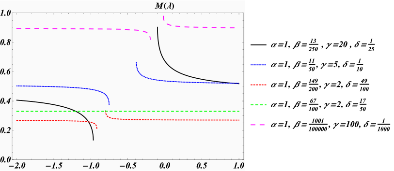
[h]

Figure 1: Modified mass $M$ as a function of $\lambda$ for $m=1$ with $\lambda\in\mathbb{R}\backslash(-0.9665,-0.0998)$, $\lambda\in\mathbb{R}\backslash(-0.7534,-0.3846)$, $\lambda\in\mathbb{R}\backslash(-0.9182,-0.8)$, $\lambda\in\mathbb{R}\backslash(-0.80709,-0.8)$ and $\lambda\in\mathbb{R}\backslash(-0.1978,-0.0200)$.

We expect to recover the Hermitian case by demanding either the position and the momentum, the position and the number operator or the momentum and the number operator to be observables. Indeed by equating any two of these masses, i.e. $\hat{M}(0)=\hat{M}(\pm 1)$ or $\hat{M}(1)=\hat{M}(-1)$, together with the constraint on the determinant of $T$ leads to the values in (12) for two of the parameters.

3.3 Adjoint constraint

Let us now also relax the constraint (22), such that $e^{\dagger}\neq\varkappa f$ and in addition allow $\alpha,\beta,\gamma,\delta\in\mathbb{C}$. Whereas in the previous subsections the construction of the eigenfunctions follows trivially from the harmonic oscillator realization in terms of modified masses and frequencies, this is less obvious for this setting. We therefore present the construction commencing by expressing the pseudo-bosons $e$ and $f$ in position space. From (8) and (14) simply follows

$$e=\frac{1}{\sqrt{2}}\left[\left(\tilde{\beta}-\tilde{\delta}\right)x+\left(\tilde{\beta}+\tilde{\delta}\right)\frac{d}{dx}\right],\quad f=\frac{1}{\sqrt{2}}\left[\left(\tilde{\gamma}-\tilde{\alpha}\right)x-\left(\tilde{\alpha}+\tilde{\gamma}\right)\frac{d}{dx}\right],$$ (31)

As we no longer need modified values for the mass and frequency we have set here $m=\omega=\hbar=1$ for simplicity. Hence, following [17], the vacua of $e$ and $f^{\dagger}$ are

$$\varphi_{0}(x)=N_{\varphi}e^{-\frac{1}{2}\,x^{2}\,\frac{\tilde{\beta}-\tilde{\delta}}{\tilde{\beta}+\tilde{\delta}}},\quad\quad\text{and\quad\quad}\Psi_{0}(x)=N_{\Psi}e^{-\frac{1}{2}\,x^{2}\,\frac{\tilde{\gamma}^{\ast}-\tilde{\alpha}^{\ast}}{\tilde{\gamma}^{\ast}+\tilde{\alpha}^{\ast}}},$$ (32)

respectively, where $N_{\varphi}$ and $N_{\Psi}$ are suitable normalization constants to be specified further below. Naturally we require

$$\mathop{\mathrm{R}e}\left(\frac{\tilde{\beta}-\tilde{\delta}}{\tilde{\beta}+\tilde{\delta}}\right)>0,\quad\quad\text{and\quad\quad}\mathop{\mathrm{R}e}\left(\frac{\tilde{\gamma}-\tilde{\alpha}}{\tilde{\gamma}+\tilde{\alpha}}\right)>0,$$ (33)

to ensure the square-integrability for both of these functions. In complete analogy to [17] we further construct the functions

$$\varphi_{n}(x) = \frac{f^{n}}{\sqrt{n!}}\varphi_{0}(x)=\frac{N_{\varphi}}{\sqrt{n!2^{n}}}\left(\frac{\tilde{\alpha}+\tilde{\gamma}}{\tilde{\beta}+\tilde{\delta}}\right)^{n/2}H_{n}\left[\frac{x}{\sqrt{(\tilde{\alpha}+\tilde{\gamma})(\tilde{\beta}+\tilde{\delta})}}\right]\,e^{-\frac{1}{2}\,x^{2}\,\frac{\tilde{\beta}-\tilde{\delta}}{\tilde{\beta}+\tilde{\delta}}},$$ (34)

$$\Psi_{n}(x) = \frac{{e^{\dagger}}^{n}}{\sqrt{n!}}\Psi_{0}(x)=\frac{N_{\Psi}}{\sqrt{n!2^{n}}}\left(\frac{\tilde{\beta}^{\ast}+\tilde{\delta}^{\ast}}{\tilde{\alpha}^{\ast}+\tilde{\gamma}^{\ast}}\right)^{n/2}H_{n}\left[\frac{x}{\sqrt{(\tilde{\alpha}^{\ast}+\tilde{\gamma}^{\ast})(\tilde{\beta}^{\ast}+\tilde{\delta}^{\ast})}}\right]\,e^{-\frac{1}{2}\,x^{2}\,\frac{\tilde{\gamma}^{\ast}-\tilde{\alpha}^{\ast}}{\tilde{\gamma}^{\ast}+\tilde{\alpha}^{\ast}}}.$$

from a repeated action of $f$ and ${e^{\dagger}}$ on the corresponding ground states in (32) for $n\geq 0$. When the constraint (33) holds these functions are square-integrable and can be used to define the sets $\mathcal{F}_{\varphi}:=\{\varphi_{n},n\geq 0\}$ and $\mathcal{F}_{\Psi}:=\{\Psi_{n},n\geq 0\}$. Applying here what was proven in [17], we deduce that $\mathcal{F}_{\varphi}$ and $\mathcal{F}_{\Psi}$ form biorthogonal bases for $\mathcal{H}$ when $\tilde{\alpha}\,\tilde{\beta}=\tilde{\gamma}\,\tilde{\delta}$, i.e. we have

$$\chi(x)=\sum_{n=0}^{\infty}\left\langle\Psi_{n},\chi\right\rangle\varphi_{n}(x)=\sum_{n=0}^{\infty}\left\langle\varphi_{n},\chi\right\rangle\Psi_{n}(x),$$ (35)

for all $\chi(x)\in\mathcal{L}^{2}(\mathbb{R)}$. Notice that $\tilde{\alpha}\,\tilde{\beta}=\tilde{\gamma}\,\tilde{\delta}$ is simply the constraint (22) when eliminating $\varkappa$, such that $h$ becomes self-adjoint. When this constraint is relaxed, i.e. $\tilde{\alpha}\,\tilde{\beta}\neq\tilde{\gamma}\,\tilde{\delta}$, the two sets still form ${\mathcal{D}}$-quasi bases, i.e. we have

$$\left\langle\chi,\xi\right\rangle=\sum_{n=0}^{\infty}\left\langle\chi,\Psi_{n}\right\rangle\left\langle\varphi_{n},\xi\right\rangle=\sum_{n=0}^{\infty}\left\langle\chi,\varphi_{n}\right\rangle\left\langle\Psi_{n},\xi\right\rangle,$$ (36)

for all $\chi,\xi\in{\mathcal{D}}$, a dense subset of $\mathcal{L}^{2}(\mathbb{R)}$ defined as follows:

$${\mathcal{D}}=\left\{\chi(x)\in\mathcal{L}^{2}(\mathbb{R)}:\,e^{\frac{1}{2}x^{2}|\tilde{\alpha}\tilde{\beta}-\tilde{\gamma}\tilde{\delta}|}\chi(x)\mathbb{\in}\mathcal{L}^{2}(\mathbb{R)}\right\}.$$ (37)

It is possible to verify that each $\Psi_{n}(x)$ is in the domain of $\eta$ while each $\varphi_{n}(x)$ is in the domain of $\eta^{-1}$, that is $\Psi_{n}(x)\in D(\eta)$ and $\varphi_{n}(x)\in D(\eta^{-1})$. We prove this as follows: By the definition of $\varphi_{n}$ we know that $\varphi_{n+1}=\frac{1}{\sqrt{n+1}}\,f\varphi_{n}$, for all $n\geq 0$. Since $\varphi_{k}\in\mathcal{L}^{2}(\mathbb{R)}$ for all $k$, we conclude that $\varphi_{n}\in D(f)$. Recalling now that $f=\eta c\eta^{-1}$, it follows that $D(f)\subseteq D(\eta^{-1})$. Hence, since $\varphi_{n}\in D(f)$ this means $\varphi_{n}\in D(\eta^{-1})$. Similarly we can check that each $\Psi_{n}\in D(\eta)$. These facts are important, since they imply that both $\eta$ and $\eta^{-1}$ are densely defined. In fact, $\eta^{-1}$ is defined on $\mathcal{L}_{\varphi}$, the linear span of the $\varphi_{n}$’s, which is dense in $\mathcal{H}$ since $\mathcal{F}_{\varphi}$ is complete (or, if $\tilde{\alpha}\,\tilde{\beta}=\tilde{\gamma}\,\tilde{\delta}$, is even a basis). Similarly, $\eta$ is defined on $\mathcal{L}_{\Psi}$, the linear span of the $\Psi_{n}$’s, which is dense in $\mathcal{H}$ since $\mathcal{F}_{\Psi}$ is complete (or, again, if $\tilde{\alpha}\,\tilde{\beta}=\tilde{\gamma}\,\tilde{\delta}$, is a basis).

More detail on this case may be found in [17].

4 Conclusions

We further investigated a particular type of pseudo-bosons that are obtainable from generalized Bogoliubov transformations [17]. We apply on them a second generalized Bogoliubov transformation satisfying certain properties and demand that it equals a particular adjoint map acting on these operators. We employ these doubly transformed operators to build a simple Hamiltonian consisting of these special pseudo-bosonic number operators.

We impose constraints on the model parameters, which we gradually relax. Choosing at first the model parameters in such a way that the Hamiltonian becomes Hermitian we found that one requires further simple constraints on the ordering of the model parameters in order to obtain a positive mass. This requirement turned out to be the same as demanding square integrability of the wave functions. As the next case we demand the adjoint map to be equivalent to the Dyson map that achieves pseudo-Hermiticity. In this setting, we obtain the typical scenario in pseudo-Hermitian systems namely a whole ray of equivalent Hermitian Hamiltonians (28) parametrized by a non-model dependent quantity, $\lambda$ in our case, entering through the similarity transformation. We found that $\lambda$ is always defined on two disjoint intervals on the real line. In the excluded parameter regime the mass becomes complex as a consequence of $\varepsilon(\lambda)$ in (24) becoming complex. Finally when relaxing all constraints we loose the proper that $\mathcal{F}_{\varphi}$ and $\mathcal{F}_{\Psi}$ form biorthogonal bases as in the Hermitian scenario, but we still obtain ${\mathcal{D}}$-quasi bases.

The main virtue of our construction lies in the reduction of the relevant transformations to the more basic bosonic ingredients. Even though the doubly Bogoliubov transformed objects are more restrictive when compared to the most general treatment, they always select out a set of feasible models. Naturally, they may be employed in other more complicated models, involving for instance cubic [22] or higher order terms in its defining Hamiltonian.

Acknowledgments: FB gratefully acknowledges financial support from City University London, from the Università di Palermo, via CORI 2014, Action D and from G.N.F.M.

References

- [1] C. M. Bender and S. Boettcher, Real Spectra in Non-Hermitian Hamiltonians Having PT Symmetry, Phys. Rev. Lett. 80, 5243–5246 (1998).
- [2] C. M. Bender, Making sense of non-Hermitian Hamiltonians, Rept. Prog. Phys. 70, 947–1018 (2007).
- [3] A. Mostafazadeh, Pseudo-Hermitian Representation of Quantum Mechanics, Int. J. Geom. Meth. Mod. Phys. 7, 1191–1306 (2010).
- [4] C. M. Bender, A. Fring, U. Guenther, and H. F. Jones, Special issue on quantum physics with non-Hermitian operators, Journal of Physics A: Mathematical and Theoretical 45(1), 010201 (2012).
- [5] Z. H. Musslimani, K. G. Makris, R. El-Ganainy, and D. N. Christodoulides, Optical Solitons in PT Periodic Potentials, Phys. Rev. Lett. 100, 030402 (2008).
- [6] K. G. Makris, R. El-Ganainy, D. N. Christodoulides, and Z. H. Musslimani, PT-symmetric optical lattices, Phys. Rev. A81, 063807(10) (2010).
- [7] A. Guo, G. J. Salamo, D. Duchesne, R. Morandotti, M. Volatier-Ravat, V. Aimez, G. A. Siviloglou, and D. Christodoulides, Observation of PT-Symmetry Breaking in Complex Optical Potentials, Phys. Rev. Lett. 103, 093902(4) (2009).
- [8] F. J. Dyson, Thermodynamic Behavior of an Ideal Ferromagnet, Phys. Rev. 102, 1230–1244 (1956).
- [9] C. M. Bender, D. C. Brody, and H. F. Jones, Extension of PT-symmetric quantum mechanics to quantum field theory with cubic interaction, Phys. Rev. D70, 025001(19) (2004).
- [10] A. Mostafazadeh, PT-symmetric cubic anharmonic oscilator as a physical model, J. Phys. A38, 6557–6570 (2005).
- [11] A. Sinha and R. Roychoudhury, Isospectral partners of a complex PT-invariant potential, Physics Letters A 301(3), 163–172 (2002).
- [12] C. Figueira de Morisson Faria and A. Fring, Time evolution of non-Hermitian Hamiltonian systems, J. Phys. A39, 9269–9289 (2006).
- [13] C. Figueira de Morisson Faria and A. Fring, Isospectral Hamiltonians from Moyal products, Czech. J. Phys. 56, 899–908 (2006).
- [14] D. P. Musumbu, H. B. Geyer, and W. D. Heiss, Choice of a metric for the non-Hermitian oscillator, J. Phys. A40, F75–F80 (2007).
- [15] P. E. G. Assis and A. Fring, Non-Hermitian Hamiltonians of Lie algebraic type, J. Phys. A42, 015203 (23p) (2009).
- [16] M. S. Swanson, Transition elements for a non-Hermitian quadratic Hamiltonian, J. Math. Phys. 45, 585–601 (2004).
- [17] F. Bagarello and A. Fring, Generalized Bogoliubov transformations versus -pseudo-bosons, Journal of Mathematical Physics 56(10), 103508 (2015).
- [18] F. Bagarello, Deformed canonical (anti-)commutation relations and non-hermitian hamiltonians, in Non-Hermitian operators in quantum physics: Mathematical aspects, F. Bagarello, J. P. Gazeau, F. H. Szafraniec and M. Znojil, Eds., (John Wiley and Sons, New Jersey) (2015).
- [19] N. N. Bogolyubov, On a new method in the theory of superconductivity, Nuovo Cim. 7, 794–805 (1958).
- [20] F. Hong-Yi and J. Vanderlinde, Generalized Bogolyubov transformation, J. Phys. A23, L1113–L1117 (1990).
- [21] F. G. Scholtz, H. B. Geyer, and F. Hahne, Quasi-Hermitian Operators in Quantum Mechanics and the Variational Principle, Ann. Phys. 213, 74–101 (1992).
- [22] P. E. G. Assis and A. Fring, Metrics and isospectral partners for the most generic cubic -symmetric non-Hermitian Hamiltonian, J. Phys. A41, 244001 (2008).