Market Dynamics of Best-Response with Lookahead

Abstract

In both general equilibrium theory and game theory, the dominant mathematical models rest on a fully rational solution concept in which every player’s action is a best-response to the actions of the other players. In both theories there is less agreement on suitable out-of-equilibrium modeling, but one attractive approach is the level $k$ model in which a level $0$ player adopts a very simple response to current conditions, a level $1$ player best-responds to a model in which others take level $0$ actions, and so forth. (This is analogous to $k$-ply exploration of game trees in AI, and to receding-horizon control in control theory.) If players have deterministic mental models with this kind of finite-level response, there is obviously no way their mental models can all be consistent. Nevertheless, there is experimental evidence that people act this way in many situations, motivating the question of what the dynamics of such interactions lead to.

We address this question in the setting of Fisher Markets with constant elasticities of substitution (CES) utilities, in the weak gross substitutes (WGS) regime. We show that despite the inconsistency of the mental models, and even if players’ models change arbitrarily from round to round, the market converges to its unique equilibrium. (We show this for both synchronous and asynchronous discrete-time updates.) Moreover, the result is computationally feasible in the sense that the convergence rate is linear, i.e., the distance to equilibrium decays exponentially fast. To the best of our knowledge, this is the first result that demonstrates, in Fisher markets, convergence at any rate for dynamics driven by a plausible model of seller incentives. Even for the simple case of (level $0$) best-response dynamics, where we observe that convergence at some rate can be derived from recent results in convex optimization, our result is the first to demonstrate a linear rate of convergence.

1 Introduction

Motivation

This paper deals with the question of why, and whether, a model of interacting strategic agents converges to equilibrium. We study this question in Fisher markets, under conditions where market equilibrium is unique and finding it is computationally tractable. Over the years and in particular recently, several game and market dynamics have been studied, but they fall short of modeling the key scenario which we attempt to address.

In particular, in game theory, dynamics are studied in the context of repeated games. Extensive form solution concepts such as subgame perfect or sequential equilibria assume that the agents unravel the entire evolution of the game and choose in advance their entire play optimally. This is likely to be computationally infeasible (e.g. [8], but see in contrast [25]). The strategies are unrealistically prescient of the distant future, contradicting experience and hindering on-the-fly adaptation to unexpected changes. Just as importantly, since the entire play is determined a-priori and an equilibrium is played throughout, such concepts do not capture out-of-equilibrium behavior (that may lead to equilibrium over time), so they are in fact a static notion.

Walrasian tâtonnement, and more generally game theoretic learning dynamics (a.k.a. no-regret dynamics), are an alternative approach. These are truly dynamic, out-of-equilibrium frameworks, that can be shown in many cases to converge to an attractive solution concept. However, the reactions of the agents have to be damped carefully for a desirable outcome to materialize; such reactions lack strategic justification (see [7] and the references therein, e.g., [26]).

Closer to our work, various formulations of bounded rationality have provided a rich basis for progress in game theory and, over the last two decades, in its algorithmic aspects. The most basic approach in this vein is best-response dynamics. Agents play myopically an optimal move at each round, assuming that the other agents will not deviate from their existing strategy. A strategy which is somewhat more sophisticated than best-response is limited-depth exploration of an extensive form game tree. This is an approach to complex games that was developed in the early days of AI (the exploration depth is sometimes called the ply of a search). Essentially the same concept is known in control theory as receding-horizon control. This is in contrast with the full-rationality approach underlying solution concepts such as the aforementioned subgame perfect or sequential equilibria.

In game theory, the idea that people compete by pursuing limited-lookahead situational analysis goes under the rubric of the level $k$ model, initiated by [43, 44] and [37]; related ideas are also known as cognitive hierarchy, higher-order rationality, and bounded depth of reasoning. The idea has been subjected to many experimental tests—see [28, 15, 16, 9, 14, 19, 18]—and has emerged with considerable support. For recent theoretical work on the model see [45, 30, 20, 24]; for a survey see [17].

In view of the above, it is important to study the dynamics and stability of markets composed of agents each of whom performs some limited lookahead and plays optimally against that forecast. Limited lookahead means that each agent $j$ has a mental model of each other agent $k$, where $k$ looks ahead some constant number of steps, and based on that chooses an optimal action (according to $j$’s perception). Based on this model, $j$ chooses a move that is optimal conditional on those other imagined actions. The paradox of endless self-reference is obvious here, and is precisely the point of the exercise: such a model does not make sense for infinitely-intelligent agents who possess perfect common knowledge of the properties of the market. But such agents do not exist. Instead, the model is consistent with experience that markets are composed of many agents who, despite having limited ability to predict the actions of others, do their best to make such a prediction and then respond optimally to their own prediction. This is a very different approach to agent choice than the “solution concept” notion on which game theory rests: Nash equilibria, correlated equilibria, the core, and so forth. In particular, one difference is that in contrast with full rationality, in the limited lookahead case the beliefs of the agents are not necessarily consistent with each other and with reality. In fact, they may even be self-inconsistent across time steps. From a purely mathematical perspective these inconsistencies might appear to be a fatal flaw. We hold differently, that this is part of the challenge of modeling out-of-equilibrium strategic play. The market is out of equilibrium because players do not have perfect models of each other, or because they are uncertain about exogenous factors a few steps into the future. We further hold that the predictive power in experiments of the level $k$ model is ample reason to study its dynamics. That is what we do here (and for a more general notion of best-response with lookahead).

Our results

This paper is devoted to studying the dynamics and stability of markets where the agents model their peers as using limited lookahead. We focus on one of the best-understood cases of general equilibrium theory, namely Fisher markets that consist of sellers of goods and buyers endowed with budgets.

In fact, we develop a general framework that shows convergence of dynamics based on limited lookahead, only requiring certain abstract conditions on the updates of the players. A concrete special case is a Fisher market in which the buyers generate demand due to utilities that exhibit constant elasticity of substitution (CES), in the weak gross substitutes (WGS) regime. (Rigorous definitions await Sections 2 and 3.) CES utilities were chosen because this setting is very well understood in the context of discrete-time tâtonnement (see [10]), and this gives us some comparative perspective. The restriction to WGS was imposed because otherwise even staying at a market equilibrium cannot be reasoned by individual sellers best-responding to the equilibrium.

Our dynamic model focuses on the sellers. Each seller controls and sets the price of a unique single good. The buyers are assumed to react instantly and myopically to current prices by adjusting their demand to optimize their utilities subject to their budgets. This assumption can be justified, for instance, by assuming that there is a large number of buyers, each contributing negligibly to the demand. Each seller is assumed to form a belief on the next move of each of the other sellers, and then to choose a price that optimizes its own profit based on this belief. We analyze a rather general belief formation process that includes, as a special case, beliefs based on assuming that the other sellers use limited lookahead. We assume neither consistency among the beliefs formed by different sellers, nor consistency among the beliefs formed by the same seller at different times. This includes as a special case, but is considerably more general than, level $k$ choices. See Figure 1. We refer to dynamics of this sort as best-response with lookahead (abbreviated BRL) dynamics.

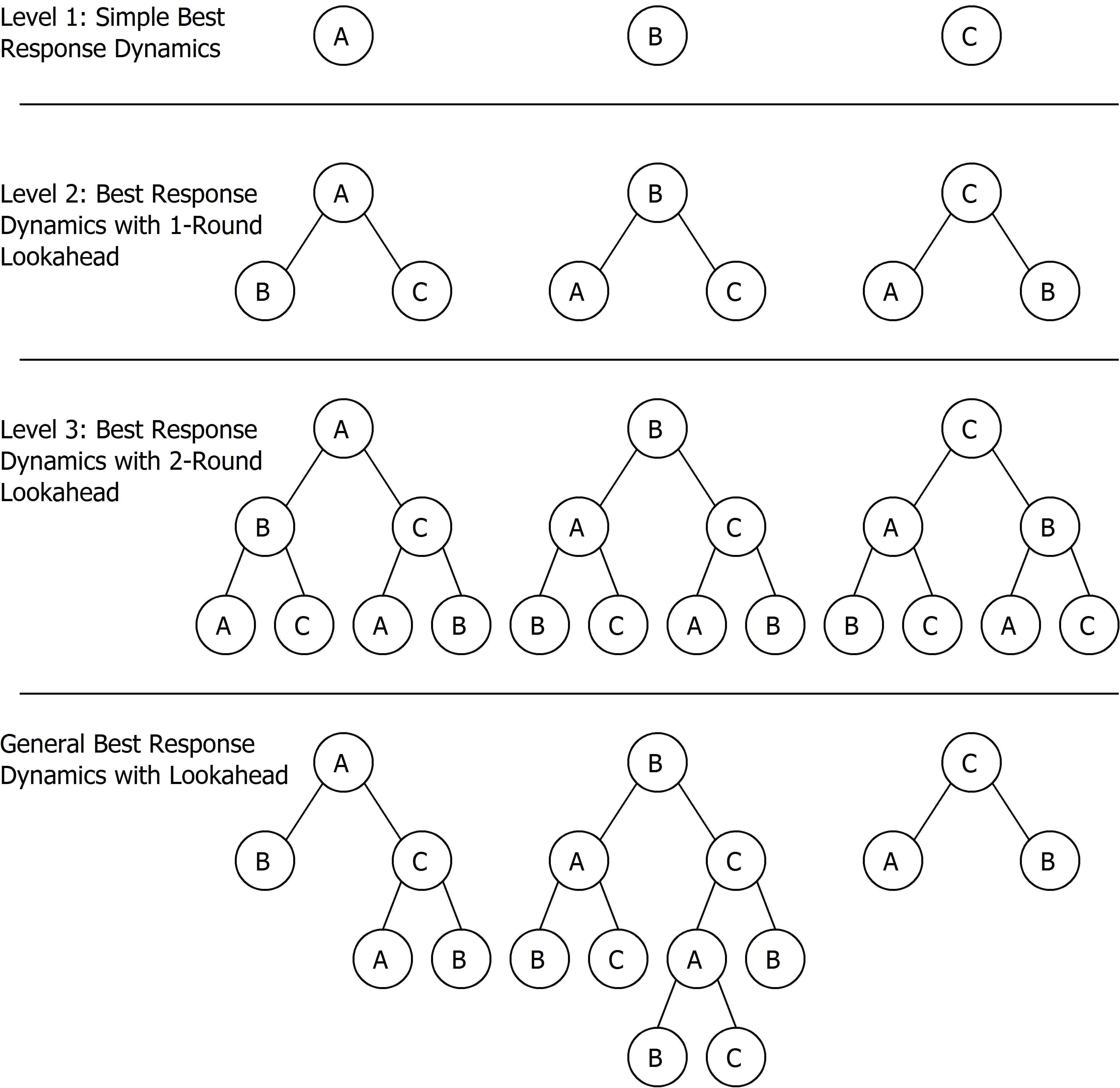
Figure 1: Various collective mental models for one round of play in a 3-seller market. A leaf (level $1$) denotes best-response dynamics. In level $2$ dynamics everyone best-responds to everyone’s best-response to current prices. Players’ beliefs can be far more complex. In the last example C plays by a level $2$ model while A and B have more elaborate mental models.

BRL dynamics, and even the special case of best-response (with no lookahead), can be quite volatile, as compared with usual tâtonnement processes, because of the absence of any damping factor. Despite the volatility and the potential inconsistency of beliefs, we show that regardless of the specifics of the beliefs formed by the agents, the dynamic converges rapidly to market equilibrium. More precisely, we analyze two versions of our process. In the synchronous case, all sellers update prices simultaneously. In this case, the distance to equilibrium decays exponentially in the number of steps (a.k.a. linear convergence). In the asynchronous case, at each time step only a subset of one or more sellers update prices. In this case, the distance to equilibrium decays exponentially in the number of epochs, where an epoch consists of time intervals in which all the sellers update at least once.

To the best of our knowledge, convergence, and definitely linear convergence, was not previously demonstrated even for the simplest version of our process, namely best-response. Our proof of convergence relies on showing that in a judiciously chosen metric (the Thompson metric), the BRL dynamics form a contraction map.

Related work

General equilibrium theory is the principal framework through which economists understand the operation of markets (see [33, 36]). It is one of the great achievements of economic theory in general and of mathematical modeling of microeconomics in particular. The theory is largely responsible for the governing paradigm that a state of equilibrium which the participants in economic exchange do not wish to deviate from individually is under mild conditions attainable [2, 32] (see also [27]), and that this is normally roughly the state of the economy. This is a paradigm that can be observed “in the field” and also reproduced in controlled experiments, and it lends credence and concreteness to the famed invisible hand metaphor.

In contrast, there is less agreement on an effective explanation as to why markets tend to reach a state of equilibrium. This is a question about the stability or out-of-equilibrium behavior of markets. It is important because in reality economic conditions are not static. They vary continually and suffer serious “shocks” occasionally. So justifying an equilibrium outcome requires a dynamic that moves an economy at disequilibrium back to a new equilibrium, and does so sufficiently quickly that the periods of disequilibrium due to fluctuations are relatively negligible (see [21]). The classical mechanism proposed to explain general equilibrium is Walrasian tâtonnement [47], a process that reacts to excess demand by raising the price and to excess supply by reducing the price. Variants of tâtonnement are known to converge to equilibrium, at least in some classes of markets including those we consider here (e.g. [41, 1, 10]). However, the classical view of tâtonnement posits the existence of an imaginary “auctioneer” who controls the process by announcing prices. Recent work on the convergence of discrete-time tâtonnement in Fisher markets attempts to present it as an in-market process in the context of the so-called ongoing markets [13, 11]. However, even this attempt requires a somewhat careful choice of the magnitude of the price adjustment which is not motivated by any agent considerations (aside from a common inexplicable passion to equilibrate the economy). Thus, the difficulty is in formulating a theory of out-of-equilibrium behavior that makes sense in terms of the incentives of the participants.

In is well-known that market equilibria in Fisher markets with CES utilities can be expressed as solutions to a convex program, first proposed by Eisenberg and Gale (see [29]). We observe that best-response dynamics (i.e., the simplest example of our setting) can, in fact, be explained as a specific implementation of coordinate descent (in the dual program). The convergence of coordinate descent was established in [46], without bounds on the rate. Recently, [40] established a sublinear convergence rate (the distance to the optimum decays linearly with the number of iterations), if the objective function satisfies some conditions. We note that the objective function of the dual Eisenberg-Gale program satisfies these conditions. Our general result shows a linear convergence rate (the distance to equilibrium decays exponentially in the number of iterations), and this holds in particular in the case of best-response. To the best of our knowledge, this is not implied by previous results.

Two recent papers consider market dynamics under strategic behavior. Both bound the fraction of optimal welfare that is guaranteed. In [5], strategic buyers play a Nash (or Bayesian) equilibrium in a market in which the sellers’ prices are determined by Walrasian tâtonnement; note that here the tâtonnement is part of the mechanism defining the game, rather than the agents’ strategies. In [6], sellers engage in best-response dynamics. In this setting the market does not actually have an equilibrium, but a fraction of the optimal welfare can be extracted by the dynamic. In both papers the market model is quite different from ours.

In the game theory setting (as opposed to markets), best-response dynamics have been studied extensively in recent years, mostly concerning bounds on the quality of the play and conditions that imply or prevent convergence to a Nash equilibrium [34, 39, 23, 22]. The paper [38] investigates conditions under which best-response is a fully rational strategy.

2 Preliminaries

The market model

We consider a Fisher market with $n$ perfectly divisible goods and $m$ buyers. Each good is initially owned by a unique seller that controls its price, and its quantity is scaled to $1$. The utility of that seller is the price times $\min\{\text{demand},1\}$. The buyers respond instantly and myopically to price changes. Thus their role in the process is to specify in a convenient way the demands for the goods at any given assignment of prices to those goods. This is done as follows. Each buyer $i$ is endowed with a positive budget $b_{i}$ and a utility function $u_{i}$ over baskets of goods $x$.

For a price vector $p$, we write $p>0$ to indicate that all the prices are strictly positive. Similarly for price vectors $p,q$, we write $p>q$ (resp. $p\geq q$) if $p_{j}>q_{j}$ (resp. $p_{j}\geq q_{j}$) for all $j$.

Given a price vector $p>0$, the demands for the goods are determined as follows. Every buyer $i$ chooses $x_{i}$ to optimize the utility function $u_{i}(x)$, subject to the budget constaint

$$\sum_{j}p_{j}x_{ij}\leq b_{i}.$$ (1)

We denote the utility maximizing allocations for prices $p$ by $x(p)$. The demand for each good $j$ at prices $p$ is $\sum_{i}x_{ij}(p)$.

Price updates

In general, a market dynamic is based on an update rule for each seller that determines its new price. The rules can then by applied synchronously to all sellers, or serially to one seller at a time in some order. We will discuss these variations later. For now, we focus on the update rules. An update rule can take into account some or all of the dynamic history leading to the current state (including the current prices), and also some internal state of the seller that takes other factors into account. We are interested in update rules that depend on the current price vector (and any other parameters), and are monotone, sub-homogeneous, price-bounded, and positive with respect to that price vector. To define these properties formally, let $F^{\iota}_{j}(p)$ denote the new price of seller $j$, given current prices $p$, and $\iota$ encoding all the other relevant parameters (if any). Then,

Definition 1 (monotonicity, sub-homogeneity, price-boundedness, positivity).

We say that:

• $F^{\iota}_{j}$ is monotone if for all pairs of price vectors $p,q$ such that $p\geq q$ coordinate-wise, $F^{\iota}_{j}(p)\geq F^{\iota}_{j}(q)$;

• $F^{\iota}_{j}$ is sub-homogeneous if for all price vectors $p$ and for all $\lambda\in(0,1)$, $F^{\iota}_{j}(\lambda p)\geq\lambda F^{\iota}_{j}(p)$, also $F^{\iota}_{j}$ is strictly sub-homogeneous iff the inequality is strict for all $p>0$;

• $F^{\iota}_{j}$ is $[p_{\min},p_{\max}]$-price-bounded if for all price vectors $p\in[p_{\min},p_{\max}]^{n}$, $F^{\iota}_{j}(p)\in[p_{\min},p_{\max}]$.

• $F^{\iota}_{j}$ is positive if $p_{\min}>0$.

For a price vector $p$ and price updates $F_{j}$ for all $j\in[n]$, we denote by $F(p)$ the price vector derived by applying the updates simultaneously to $p$. We say that $F$ has a property (e.g., is monotone) if all of its components have this property.

Lemma 2.

Fix $p_{\min},p_{\max}$, and suppose that $F:[p_{\min},p_{\max}]^{n}\rightarrow[p_{\min},p_{\max}]^{n}$ and $g:[p_{\min},p_{\max}]^{n}\rightarrow[p_{\min},p_{\max}]$ are both monotone, sub-homogeneous, and $[p_{\min},p_{\max}]$-price bounded updates. Then so is $g\circ F$. Moreover, if $g$ is strictly sub-homogeneous and $F$ is positive, then $g\circ F$ is also strictly sub-homogeneous.

Proof.

By the monotonicity of $F$, if $p\geq q$ coordinate-wise, then $F(p)\geq F(q)$ coordinate-wise. Therefore, by the monotonicity of $g$, we have that $g(F(p))\geq g(F(q))$. Next, $g(F(\lambda p))\geq g(\lambda F(p))\geq\lambda g(F(p))$, where the first inequality uses the monotonicity of $g$ and the sub-homogeneity of $F$, and the second inequality uses the sub-homogeneity of $g$. Moreover, if $g$ is strictly sub-homogeneous, then the second inequality is strict if $F(p)>0$, which is implied when $p>0$ by the assumption that $F$ is positive. Finally, using the price boundedness of both $F$ and $g$, if $p\in[p_{\min},p_{\max}]^{n}$, then $F(p)\in[p_{\min},p_{\max}]^{n}$, so $g(F(p))\in[p_{\min},p_{\max}]$. ∎

Belief formation

We consider dynamics where each seller updates its price according to a belief of which prices the other sellers will set in the next step. The beliefs that are formed by different sellers or by the same seller at different times need not be consistent. We show that despite this inconsistency, the dynamics still converge to equilibrium, assuming that the ingredients satisfy certain properties. In general, a belief $\pi$ is a function that maps a pair $(p,\iota)$, where $p$ is the current price vector and $\iota$ is the internal state of the seller, to the believed price vector.

We now discuss a rather general framework of forming such beliefs. This framework in particular enables the sellers to form level $k$ best-response beliefs, and more general best-response beliefs. We haven’t yet formally defined “best-response”, but for now it suffices to assume that there is at our disposal a price update called best-response. The details of best-response update are discussed in Section 3. Also, in order to get some intuition on the following explanation, it might be useful to visualize the trees in the bottom example in Figure 1.

We explain how seller $j$ forms a belief $\pi=\pi^{\iota}$. The idea is that seller $j$ has, for every other seller $k$, a mental model $\iota_{k}$ of the update rule that $k$ employs, and $\pi_{k}$ is simply the price that $\iota_{k}$ generates. Of course, in order to form $\iota_{k}$, seller $j$ must also imagine seller $k$’s mental models for all $k^{\prime}\neq k$ (this includes $j$). So, we define inductively a set of possible mental models of seller updates, and seller $j$ simply picks each $\iota_{k}$ from this set. The set ${\cal M}$ of mental models consists of levels; ${\cal M}=\bigcup_{s=0}^{\infty}{\cal M}_{s}$. They are defined inductively as follows. The base case, level $0$, is ${\cal M}_{0}$ that contains a single model of staying put at the current price. Inductively, a mental model or belief $\iota$ for player $j$ is formed by selecting any $\iota_{k_{1}},\ldots,\iota_{k_{n}}$ (but there is no $\iota_{j}$); the price update defined by this mental model is player $j$’s best-response to the prices generated by all the other players if they act with the assigned mental models on the basis of the current prices. The level of $\iota$ is one more than the maximum level of $\iota_{k_{1}},\ldots,\iota_{k_{n}}$.

We note in passing that beliefs thus formed, implicitly model sellers with epistemic assumptions that they are a bit smarter than their peers—every seller $j$ updates with one extra step beyond the maximum number of steps used in $j$’s mental model $\iota$. Of course, such beliefs cannot possibly be consistent among sellers (unless they are children in Lake Wobegon).

The following lemma states the desired properties of belief formation.

Lemma 3.

Fix $p_{\min},p_{\max}$. Suppose that best-response is monotone, sub-homogeneous, $[p_{\min},p_{\max}]$-price bounded and positive. Further suppose that seller $j$ uses a monotone, strictly sub-homogeneous, and $[p_{\min},p_{\max}]$-price bounded update function $F_{j}$, and given current prices $p$, updates to $F^{\iota}_{j}(p)=F_{j}(\pi^{\iota}(p))$. Then, $F^{\iota}_{j}$ is monotone, strictly sub-homogeneous, and $[p_{\min},p_{\max}]$-price-bounded.

Proof.

Since staying put at the current price is monotone, sub-homogeneous, and $[p_{\min},p_{\max}]$-price-bounded, a simple induction on $s$ using Lemma 2 shows that $\pi^{\iota}$ is monotone, sub-homogeneous, and $[p_{\min},p_{\max}]$-price-bounded. One more application of Lemma 2 gives the desired properties of $F^{\iota}_{j}$. ∎

3 Concrete case of CES-WGS markets

CES utilities

These are utility functions of the form

$$u_{i}(x)=\left(\sum_{j}\left(c_{ij}x_{ij}\right)^{\rho}\right)^{\frac{1}{\rho}},$$ (2)

where $x_{ij}$ denotes the quantity of good $j$ that buyer $i$ purchased. The parameter $\rho\in(-\infty,0)\cup(0,1)$ is assumed, for simplicity, to be uniform for all buyers. These utility functions are known as constant elasticity of substitution (CES) utilities. When $\rho\in(0,1)$, the goods are weak gross substitutes (WGS). In the case of $\rho\in(-\infty,0)$, the goods are complementary.

For CES utilities, the utility-maximizing allocations are given explicitly by the equation

$$x_{ij}(p)=\frac{b_{i}}{p_{j}}\cdot\frac{\left(c_{ij}/p_{j}\right)^{\epsilon}}{\sum_{k}\left(c_{ik}/p_{k}\right)^{\epsilon}},$$ (3)

where $\epsilon=\frac{\rho}{1-\rho}$. Notice that if $\rho\in(0,1)$, then $\epsilon\in(0,\infty)$. In this case, the demand satisfies the following property.

Lemma 4.

Let the utilities be CES in the WGS regime. Fix a price vector $p$ and a good $j$. Consider all price vectors $p^{\prime}$ with the property that for all $k\neq j$, $p^{\prime}_{k}=p_{k}$. Among these price vectors, the total desired spending $\sum_{i}x_{ij}(p^{\prime})\cdot p^{\prime}_{j}$ on good $j$ is monotonically decreasing in $p^{\prime}_{j}$.

Proof.

Using Equation (3), the total desired spending on $j$ is given by the equation

$$\sum_{i}x_{ij}(p^{\prime})\cdot p^{\prime}_{j}=\sum_{i}b_{i}\cdot\frac{\left(c_{ij}/p^{\prime}_{j}\right)^{\epsilon}}{\left(c_{ij}/p^{\prime}_{j}\right)^{\epsilon}+\sum_{k\neq j}\left(c_{ik}/p_{k}\right)^{\epsilon}}.$$

The derivative of the right-hand side with respect to $p^{\prime}_{j}$ is

$$-\epsilon\cdot\sum_{i}\frac{b_{i}}{p^{\prime}_{j}}\cdot\left(\left(\frac{\left(c_{ij}/p^{\prime}_{j}\right)^{\epsilon}}{\left(c_{ij}/p^{\prime}_{j}\right)^{\epsilon}+\sum_{k\neq j}\left(c_{ik}/p_{k}\right)^{\epsilon}}\right)-\left(\frac{\left(c_{ij}/p^{\prime}_{j}\right)^{\epsilon}}{\left(c_{ij}/p^{\prime}_{j}\right)^{\epsilon}+\sum_{k\neq j}\left(c_{ik}/p_{k}\right)^{\epsilon}}\right)^{2}\right).$$

This expression is negative, because $\frac{\left(c_{ij}/p^{\prime}_{j}\right)^{\epsilon}}{\left(c_{ij}/p^{\prime}_{j}\right)^{\epsilon}+\sum_{k\neq j}\left(c_{ik}/p_{k}\right)^{\epsilon}}<1$. ∎

Corollary 5.

Using the same notation as in Lemma 4, the profit $\min\left\{\sum_{i}x_{ij}(p^{\prime}),1\right\}\cdot p^{\prime}_{j}$ of seller $j$ is maximized at the price $p^{\prime}_{j}$ for which the demand $\sum_{i}x_{ij}(p^{\prime})$ equals $1$.

Proof.

By Equation (3), the demand $\sum_{i}x_{ij}(p^{\prime})$ decreases monotonically in $p^{\prime}_{j}$. By Lemma 4, also the desired spending decreases monotonically in $p^{\prime}_{j}$. Therefore, the profit is maximized at the lowest price for which the demand is at most $1$ (lowering the price further will not increase the quantity sold beyond the initial endowment). ∎

Best-response updates

In standard best-response dynamics, each seller updates its price to maximize its revenue given the current prices of the other players. In the particular setting of demand that is generated by CES utilities in the WGS regime, a seller $j$ maximizes profit by setting the price $p_{j}$ to clear the market for good $j$ (by Corollary 5). I.e., if the current price vector is $p$, the seller chooses a new price $F_{j}(p)$ for good $j$, so that

$$\sum_{i=1}^{m}x_{ij}(p^{\prime})=1,$$ (4)

where $p^{\prime}_{j}=F_{j}(p)$, and for all $k\neq j$, $p^{\prime}_{k}=p_{k}$. More explicitly, seller $j$ best-responds by solving for $p^{\prime}_{j}$ the equation

$$p^{\prime}_{j}=\sum_{i=1}^{m}b_{i}\cdot\frac{\left(c_{ij}/p^{\prime}_{j}\right)^{\epsilon}}{\sum_{k\neq j}\left(c_{ik}/p_{k}\right)^{\epsilon}+\left(c_{ij}/p^{\prime}_{j}\right)^{\epsilon}}.$$ (5)

Notice that the right-hand side of Equation (5) is simply the total spending of all the buyers on good $j$ when this good’s price is $p^{\prime}_{j}$ and the other prices are given by the vector $p$.

Lemma 6.

For CES utilities with $\rho\in(0,1)$, best-response updates $F_{j}$ are monotone, strictly sub-homogeneous, positive, and $[p_{\min},p_{\max}]$-price-bounded for some $p_{\min}=p_{\min}(b,c,\rho)>0$ and $p_{max}=p_{\max}(b)$.

Proof.

We begin with monotonicity. Consider two price vectors $p\geq q$, and let $p^{\prime}_{j}=F_{j}(p)$ and let $q^{\prime}_{j}=F_{j}(q)$. Consider the function

$$g(\alpha,p)=\alpha-\sum_{i=1}^{m}b_{i}\cdot\frac{\left(c_{ij}/\alpha\right)^{\epsilon}}{\sum_{k\neq j}\left(c_{ik}/p_{k}\right)^{\epsilon}+\left(c_{ij}/\alpha\right)^{\epsilon}}.$$

In other words, $g(\alpha,p)$ is $\alpha$ minus the total spending of all the buyers on good $j$ when the price of good $j$ is $\alpha$ and the other prices are given by the vector $p$ (thus, $g(\alpha,p)=0$ iff $\alpha=F_{j}(p)$). We have that $g(p^{\prime}_{j},p)=g(q^{\prime}_{j},q)=0$. Notice that for any $k$, increasing $p_{k}$ decreases $g(\alpha,p)$. On the other hand, $g(\alpha,p)$ increases as $\alpha$ increases (an immediate consequence of Lemma 4). Thus, $g(p^{\prime}_{j},q)\geq 0$. If $g(\alpha,q)=0\leq g(p^{\prime}_{j},q)$, then it must be that $\alpha\leq p^{\prime}_{j}$. Thus $q^{\prime}_{j}\leq p^{\prime}_{j}$.

Next we prove sub-homogeneity. Let $p^{\prime}_{j}=F_{j}(p)$. Then,

$$g(\lambda p^{\prime}_{j},\lambda p)=\lambda p^{\prime}_{j}-\sum_{i}b_{i}\cdot\frac{\left(c_{ij}/p^{\prime}_{j}\right)^{\epsilon}}{\sum_{k\neq j}\left(c_{ik}/p_{k}\right)^{\epsilon}+\left(c_{ij}/p^{\prime}_{j}\right)^{\epsilon}}=g(p^{\prime}_{j},p)-(1-\lambda)\cdot p^{\prime}_{j}\leq 0.$$

Thus, by the monotonicity of $g$ in $\alpha$, if $g(\alpha,\lambda p)=0\geq g(\lambda p^{\prime}_{j},\lambda p)$, then $\alpha\geq\lambda p^{\prime}_{j}$. Finally, if all the entries of $p$ are strictly positive, then $p^{\prime}_{j}>0$, so $g(\lambda p^{\prime}_{j},\lambda p)<0$ and therefore $g(\alpha,\lambda p)=0$ implies that $\alpha>\lambda p^{\prime}_{j}$.

Finally, we show price-boundedness. As before, let $p^{\prime}_{j}=F_{j}(p)$. For the upper bound, notice that if $p_{j}>\sum_{i}b_{i}$ then the total demand for good $j$ must be less than $1$, regardless of the other prices. So we can simply set $p_{\max}=\sum_{i}b_{i}$. For the lower bound, consider any buyer $i$ with $c_{ij}>0$. Consider the situation where all the entries of $p$ are at least $p_{\min}$, and the price of good $j$ is $q_{j}<p_{\min}$ (we will specify $p_{\min}$ shortly). The demand that $i$ has for good $j$ in this situation is

$$\frac{b_{i}}{q_{j}}\cdot\frac{\left(c_{ij}/q_{j}\right)^{\epsilon}}{\sum_{k\neq j}\left(c_{ik}/p_{k}\right)^{\epsilon}+\left(c_{ij}/q_{j}\right)^{\epsilon}}>\frac{C_{ij}}{p_{\min}},$$

where $C_{ij}=\frac{b_{i}\cdot c_{ij}^{\epsilon}}{\sum_{k}c_{ik}^{\epsilon}}$. Set $p_{\min}=\min\{1/C_{ij}:\ c_{ij}>0\}$. The demand that $i$ alone generates for good $j$ is more than $1$, so $q_{j}\neq p^{\prime}_{j}$. Thus, we must have $p^{\prime}_{j}\geq p_{\min}$. Given the value of $p_{\min}$, this shows also positivity. ∎

Best-response with lookahead (BRL) beliefs

In these dynamics, each seller best-responds to a belief (a mental model) of what the other sellers plan to do. We already discussed a general framework of forming beliefs. Now that we have defined best-response updates, Lemma 3 immediately implies the following corollary.

Corollary 7.

Let $p_{\min},p_{\max}$ be as stipulated by Lemma 6. Suppose that a price update $F_{j}$ that seller $j$ applies to a price vector $p\in[p_{\min},p_{\max}]^{n}$ is a best-response (as defined in this section) to a belief $\pi=\pi^{\iota}(p)$ that was generated by a mental model $\iota\in{\cal M}^{n-1}$ (using best-response as defined in this section). Then $F_{j}$ is monotone, strictly sub-homogeneous, and $[p_{\min},p_{\max}]$-price-bounded.

4 Synchronous Dynamics

Our main tool for proving convergence of BRL dynamics is the following theorem. Before stating the theorem, we require a definition.

Definition 8.

Consider the set ${\mathbb{R}}_{++}^{n}\subset{\mathbb{R}}^{n}$ of vectors with strictly positive coordinates. The Thompson metric $d$ on ${\mathbb{R}}_{++}^{n}$ (see [31]) is defined as follows. For $x,y\in{\mathbb{R}}_{++}^{n}$,

$$d(x,y)=\max_{i}\left|\log\frac{x_{i}}{y_{i}}\right|=\|\log x-\log y\|_{\infty},$$

where $\log x$ means the vector of logarithms of the entries of $x$.

The following Lemma shows how this metric is related to the standard $\ell_{2}$ and $\ell_{\infty}$ metrics.

Lemma 9.

Let $p^{a},p^{b}\in[p_{\min},p_{\max}]^{n}$ with $0<p_{\min}<p_{\max}$. Then, we have

$$\left\|{p^{a}-p^{b}}\right\|_{\infty}\leq\frac{\left({p_{\max}}\right)^{2}}{p_{\min}}d\left({p^{a},p^{b}}\right)$$

$$\left\|{p^{a}-p^{b}}\right\|_{2}\leq\sqrt{n}\frac{\left({p_{\max}}\right)^{2}}{p_{\min}}d\left({p^{a},p^{b}}\right)$$

Proof.

For each $i$, we have

$$\left|{p^{a}_{i}-p^{b}_{i}}\right|\leq p_{\max}\left|{\frac{p^{a}_{i}}{p^{b}_{i}}-1}\right|\leq p_{\max}\left({\exp\left({d\left({p^{a},p^{b}}\right)}\right)-1}\right)$$

The function $f\left({t}\right)=\exp\left({t}\right)-1-\kappa t$ is non-increasing on the interval $[0,\log\left({\kappa}\right)]$ for every $\kappa>0$ and evaluates to $0$ at $t=0$. Hence $\exp\left({t}\right)-1\leq\kappa t$ for every $t\in[0,\log\left({\kappa}\right)]$.

Since $d\left({p^{a},p^{b}}\right)\leq\log\left({\frac{p_{\max}}{p_{\min}}}\right)$, we can choose $\kappa=\frac{p_{\max}}{p_{\min}}$ and conclude that

$$\exp\left({d\left({p^{a},p^{b}}\right)}\right)-1\leq\frac{p_{\max}}{p_{\min}}d\left({p^{a},p^{b}}\right)$$

Thus, we have

$$\left|{p^{a}_{i}-p^{b}_{i}}\right|\leq p_{\max}\frac{p_{\max}}{p_{\min}}d\left({p^{a},p^{b}}\right)=\frac{\left({p_{\max}}\right)^{2}}{p_{\min}}d\left({p^{a},p^{b}}\right)$$

Since the bound holds for each $i$, it holds for the $\infty$ norm as well. The $2$-norm bound simply uses the fact that the $2$ norm is at most $\sqrt{n}$ times the infinity norm. ∎

Theorem 10.

Let $0<p_{\min}\leq p_{\max}<\infty$. If $F:[p_{\min},p_{\max}]^{n}\rightarrow[p_{\min},p_{\max}]^{n}$ is monotone and strictly sub-homogeneous, then it is a contraction with respect to the Thompson metric $d$. Also, if we require merely sub-homogeneity, rather than strict sub-homogeneity, then $F$ is non-expanding with respect to $d$.

Proof.

By assumption $F$ is $[p_{\min},p_{\max}]$-price-bounded. Fix $p,q\in[p_{\min},p_{\max}]^{n}$. Let $\eta=e^{d(p,q)}$. Then, we have $p\geq\frac{1}{\eta}\cdot q$ and $q\geq\frac{1}{\eta}\cdot p$. We get that

$$F(p)\geq F\left(\frac{1}{\eta}\cdot q\right)>\frac{1}{\eta}\cdot F(q),$$

where the first inequality uses monotonicity and the second inequality uses strict sub-homogeneity. Similarly,

$$F(q)>\frac{1}{\eta}\cdot F(p).$$

Thus, $d(F(p),F(q))<\log\eta=d(p,q)$ for all $p,q\in[p_{\min},p_{\max}]^{n}$. Define

$$h(\xi)=\sup\{d(F(p),F(q))-\xi\cdot d(p,q):\ p,q\in[p_{\min},p_{\max}]^{n}\}.$$

Since $[p_{\min},p_{\max}]^{n}$ is a compact set, $h(1)<0$. As $h$ is continuous, there exists $\xi\in(0,1)$ such that $h(\xi)<0$. Thus, $F$ is a contraction mapping with a contraction constant $\xi<1$. Finally, if we replace strict sub-homogeneity by sub-homogeneity, then all the strict inequalities above become weak inequalities, so we get that $d(F(p),F(q))\leq d(p,q)$, as stipulated. ∎

By Lemma 6, we immediately get the following corollary.

Corollary 11.

An update that consists of all sellers best-responding to the current price $p$ is a contraction. We denote its contraction constant by $\xi_{\operatorname{br}}<1$.

We say that a set ${\cal F}$ of price vector updates is contracting if all its elements are contractions and there is a uniform upper bound $<1$ on the contraction constants. We have the following corollary of Theorem 10.

Corollary 12.

Let ${\cal F}$ be a set of price vector updates where each $F\in{\cal F}$ is generated by all the sellers forming beliefs that satisfy the conditions of Lemma 3, then best-responding to those beliefs. Then, ${\cal F}$ is contracting, with uniform bound $\leq\xi_{\operatorname{br}}$.

Proof.

Clearly, combining Lemmas 3 and 6 with Theorem 10 proves that every $F\in{\cal F}$ is a contraction. So in order to complete the proof, we need to show that the contraction constant is at most $\xi_{\operatorname{br}}$. Let $B_{j}$ denote the best-response price update of seller $j$. Notice that by the definition of $\xi_{\operatorname{br}}$, for every $p,q\in[p_{\min},p_{\max}]^{n}$, $p\neq q$, and for every $i,j\in[n]$,

$$\frac{|\log(B_{j}(p)/B_{j}(q))|}{|\log(p_{i}/q_{i})|}\leq\xi_{\operatorname{br}}.$$

Let $\pi^{j}$ denote the belief (a mapping between price vectors) that is used by $j$ in the update $F_{j}$. I.e., $F_{j}(p)=B_{j}(\pi^{j}(p))$. Notice that by our assumptions on $\pi^{j}$ and Theorem 10, $\pi^{j}$ is non-expanding. In particular, for every $p,q\in[p_{\min},p_{\max}]^{n}$, $p\neq q$, and for every $i,k\in[n]$,

$$\frac{|\log(\pi^{j}_{k}(p)/\pi^{j}_{k}(q))|}{|\log(p_{i}/q_{i})|}\leq 1.$$

Thus, we have that for every $p,q\in[p_{\min},p_{\max}]^{n}$, $p\neq q$, and for every $i,j,k\in[n]$,

$$\frac{|\log(F_{j}(p)/F_{j}(q))|}{|\log(p_{i}/q_{i})|}=\frac{|\log(B_{j}(\pi^{j}(p))/B_{j}(\pi^{j}(q)))|}{|\log(\pi^{j}_{k}(p)/\pi^{j}_{k}(q))|}\cdot\frac{|\log(\pi^{j}_{k}(p)/\pi^{j}_{k}(q))|}{|\log(p_{i}/q_{i})|}\leq\xi_{\operatorname{br}}\cdot 1=\xi_{\operatorname{br}},$$

which completes the proof. ∎

We need an extra property to guarantee convergence to equilibrium.

Definition 13 (local stability).

We say that a set of price vector updates ${\cal F}$ is stable if the following holds for every $F\in{\cal F}$: If $p^{\ast}$ is a vector of equilibrium prices, then $F(p^{\ast})=p^{\ast}$.

Our main result is the following convergence theorem.

Theorem 14.

Fix $p_{\min},p_{\max}$. Let ${\cal F}$ be a contracting and stable set of price vector updates, where all $F\in{\cal F}$ are monotone, strictly sub-homogeneous, and $[p_{\min},p_{\max}]$-price-bounded. Consider the dynamic $p^{t+1}=F^{t}(p^{t})$, where the choice of $F^{t}\in{\cal F}$ is arbitrary. Then, with initial price vector $p^{0}\in[p_{\min},p_{\max}]^{n}$, the dynamic converges to an equilibrium point (which must be unique in this case). Moreover, the rate of convergence is linear (i.e., the distance to equilibrium decays exponentially fast in the number of time steps).

Proof.

Let $d$ be the Thompson metric on $[p_{\min},p_{\max}]^{n}$. Consider an equilibrium point $p^{*}$. By the stability of ${\cal F}$, for all $t$, $F^{t}(p^{*})=p^{*}$. By the fact that ${\cal F}$ is contracting, there exists $\xi_{\max}<1$ such that for all $t$, $F^{t}$ is a $\xi_{\max}$-contraction. Therefore,

$$d(p^{t+1},p^{*})=d(F^{t}(p^{t}),F^{t}(p^{*}))\leq\xi_{\max}\cdot d(p^{t},p^{*}).$$

Inductively, for every $T\geq 0$,

$$d(p^{T},p^{*})\leq\left(\xi_{\max}\right)^{T}d(p^{0},p^{*}).$$

This completes the proof. ∎

Corollary 15.

If the buyer utilities are CES with $\rho>0$, then synchronous best-response dynamics, as well as BRL dynamics that satisfy the conditions of Corollary 7, both converge to equilibrium at a linear rate.

Corollary 16.

Let $\mathcal{F}$ satisfy the assumptions of theorem 14. Let $p^{\ast}$ denote the vector of equilibrium prices and $p^{0}$ the initial price vector. After $T$ steps of synchronous price updates, let $p^{T}$ denote the resulting price vector. Then,

$${\|p^{T}-p^{\ast}\|}_{\infty}=\max_{i}|p_{i}-p^{\ast}_{i}|\leq\frac{\left({p_{\max}}\right)^{2}}{p_{\min}}d\left({p^{0},p^{\ast}}\right)\left({\zeta_{\max}}\right)^{T}$$

$${\|p^{T}-p^{\ast}\|}_{2}\leq\sqrt{n}\frac{\left({p_{\max}}\right)^{2}}{p_{\min}}d\left({p^{0},p^{\ast}}\right)\left({\zeta_{\max}}\right)^{T}$$

Proof.

Apply lemma 9 to theorem 14. ∎

5 Asynchronous Dynamics

We consider dynamics where each seller updates its price at its own varying rate. Thus, at any given time, only a subset of the sellers update their price. Adopting the notation from the previous section, we can formally define the dynamic by allowing some, but not all, of the coordinates of the price vector updates $F^{t}$ to be the identity map. The other coordinates are required to satisfy the same conditions that are stated in Theorem 14. We further require that no seller stays put with no update forever. Thus we can partition the time line into epochs. An epoch ends when all the prices are updated at least once, and a new epoch begins in the next time step.

Theorem 17.

Under the assumptions stated above, the dynamic, starting at initial state $p^{0}\in[p_{\min},p_{\max}]^{n}$, converges to the unique equilibrium point. The rate of convergence, measured by the number of epochs, is linear, i.e., the distance to equilibrium decays exponentially fast in the number of epochs.

Proof.

In an epoch, we can think of the last update of each seller as being applied to the price vector in the beginning of the epoch, and based on a belief that takes into account all the previous updates in the epoch. So replace the asynchronous process by a synchronous process where time steps are epochs and price updates map the prices in the beginning of an epoch to the prices at the end of an epoch. The claim follows by applying Lemma 3 and Theorem 14. ∎

Corollary 18.

If the buyer utilities are CES with $\rho>0$, then asynchronous best-response dynamics, as well as asynchronous BRL dynamics, both converge to equilibrium at a linear rate, when measured against the number of epochs. By lemma 9, the linear convergence holds in the Thompson metric $d$, the $\ell_{2}$ and the $\ell_{\infty}$ metrics.

References

- [1] K. J. Arrow, H. D. Block, and L. Hurwicz. On the stability of the competitive equilibrium: II. Econometrica, 27(1):82–109, 1959.
- [2] K. J. Arrow and G. Debreu. Existence of equilibrium for a competitive economy. Econometrica, 22:265–290, 1954.
- [3] V. Auletta, D. Ferraioli, F. Pasquale, P. Penna, and G. Persiano. Convergence to equilibrium of logit dynamics for strategic games. Algorithmica, pages 1–33, 2015.
- [4] B. Awerbuch, Y. Azar, A. Epstein, V. S. Mirrkoni, and A. Skopalik. Fast convergence to nearly optimal solutions in potential games. In Proc. of the 9th ACM Conf. on Electronic Commerce, pages 264–273, 2008.
- [5] M. Babaioff, B. Lucier, N. Nisan, and R. Paes Leme. On the efficiency of the walrasian mechanism. In Proceedings of the Fifteenth ACM Conference on Economics and Computation, EC ’14, pages 783–800, New York, NY, USA, 2014. ACM.
- [6] M. Babaioff, R. Paes Leme, and B. Sivan. Price competition, fluctuations and welfare guarantees. In Proceedings of the Sixteenth ACM Conference on Economics and Computation, EC ’15, pages 759–776, New York, NY, USA, 2015. ACM.
- [7] A. Blum and Y. Mansour. Learning, regret minimization, and equilibria. In N. Nisan, T. Roughgarden, E. Tardos, and V. V. Vazirani, editors, Algorithmic Game Theory, pages 79–102, 2007.
- [8] C. Borgs, J. T. Chayes, N. Immorlica, A. T. Kalai, V. S. Mirrokni, and C. H. Papadimitriou. The myth of the folk theorem. Games and Economic Behavior, 70(1):34–43, 2010.
- [9] C. F. Camerer, T.-H. Ho, and J.-K. Chong. A cognitive hierarchy model of games. Quarterly Journal of Economics, 119(3):861–898, 2004.
- [10] Y. K. Cheung, R. Cole, and N. R. Devanur. Tatonnement beyond gross substitutes?: gradient descent to the rescue. In Proc. of the 45th Ann. ACM Symp. on Theory of Computing, pages 191–200, 2013.
- [11] Y. K. Cheung, R. Cole, and A. Rastogi. Tatonnement in ongoing markets of complementary goods. In Proc. of the 13th Ann. ACM Conf. on Electronic Commerce, pages 337–354, 2012.
- [12] S. Chien and A. Sinclair. Convergence to approximate nash equilibria in congestion games. Games and Economic Behavior, 71(2):315–327, 2011.
- [13] R. Cole and L. Fleischer. Fast-converging tatonnement algorithms for one-time and ongoing market problems. In Proc. of the 40th Ann. ACM Symp. on Theory of Computing, pages 315–324, 2008.
- [14] M. A. Costa-Gomes and V. P. Crawford. Cognition and behavior in two-person guessing games: An experimental study. American Economic Review, 96(5):1737–1768, 2006.
- [15] M. A. Costa-Gomes, V. P. Crawford, and B. Broseta. Cognition and behavior in normal-form games: An experimental study. Econometrica, 69(5):1193–1235, 2001.
- [16] V. P. Crawford. Lying for strategic advantage: Rational and boundedly rational misrepresentation of intentions. American Economic Review, 93(1):133–149, 2003.
- [17] V. P. Crawford, M. A. Costa-Gomes, and N. Iriberri. Structural models of non-equilibrium strategic thinking: Theory, evidence, and applications. Journal of Economic Literature, 51(1):5–62, 2013.
- [18] V. P. Crawford and N. Iriberri. Fatal attraction: Salience, naïveté, and sophistication in experimental “hide-and-seek” games. American Economic Review, 97(5):1731–1750, 2007.
- [19] V. P. Crawford and N. Iriberri. Level-k auctions: Can a non-equilibrium model of strategic thinking explain the winner’s curse and overbidding in private-value auctions? Econometrica, 75(6):1721–1770, 2007.
- [20] G. de Clippel, R. Saran, and R. Serrano. Mechanism design with bounded depth of reasoning and small modeling mistakes. Working Papers 2014-7, Brown University, Department of Economics, 2014. Downloaded Oct. 28, 2015.
- [21] H. Dixon. Equilibrium and explanation. In J. Creedy, editor, The Foundations of Economic Thought, pages 356–394. Blackwell, 1990.
- [22] R. Engelberg, A. Fabrikant, M. Schapira, and D. Wajc. Best-response dynamics out of sync: Complexity and characterization. In Proceedings of the Fourteenth ACM Conference on Electronic Commerce, EC ’13, pages 379–396, New York, NY, USA, 2013. ACM.
- [23] A. Fanelli, M. Flammini, and L. Moscardelli. The speed of convergence in congestion games under best-response dynamics. ACM Trans. Algorithms, 8(3):25:1–25:15, July 2012.
- [24] O. Gorelkina. The expected externality mechanism in a level-k environment. MPI Collective Goods Preprint, No. 2015/3. Available at http://dx.doi.org/10.2139/ssrn.2550085; downloaded Oct. 28, 2015., 2015.
- [25] J. Y. Halpern, R. Pass, and L. Seeman. Not just an empty threat: Subgame-perfect equilibrium in repeated games played by computationally bounded players. In Proc. of the 10th Int’l Conf. on Web and Internet Economics, pages 249–262, 2014.
- [26] S. Hart and A. Mas-Colell. A simple adaptive procedure leading to correlated equilibrium. Econometrica, 68:1127–1150, 2000.
- [27] W. Hildenbrand. An exposition of Wald’s existence proof. In E. Dierker and K. Sigmund, editors, Karl Menger, pages 51–61. Springer, 1998.
- [28] T.-H. Ho, C. Camerer, and K. Weigelt. Iterated dominance and iterated best response in experimental ‘p-beauty contests’. American Economic Review, 88(4):947–969, 1998.
- [29] K. Jain and V. V. Vazirani. Eisenberg-gale markets: Algorithms and game-theoretic properties. Games and Economic Behavior, 70(1):84–106, 2010.
- [30] T. Kneeland. Identifying higher-order rationality. Econometrica, 83(5):2065–2079, 2015.
- [31] B. Lemmens and R. Nussbaum. Nonlinear Perron-Frobenius Theory. Cambridge University Press, 2012. Cambridge Books Online.
- [32] L. McKenzie. On equilibrium in Graham’s model of world trade and other competitive systems. Econometrica, 22:147–161, 1954.
- [33] L. W. McKenzie. Classical general equilibrium theory. MIT Press, 2002.
- [34] V. S. Mirrokni and A. Vetta. Convergence issues in competitive games. In K. Jansen, S. Khanna, J. D. P. Rolim, and D. Ron, editors, Proceedings APPROX and RANDOM, LNCS 3122, pages 183–194. Springer, 2004.
- [35] D. Monderer and L. S. Shapley. Potential games. Games and Economic Behavior, 14(1):124–143, 1996.
- [36] A. Mukherji. An introduction to general equilibrium analysis. Oxford U Press, 2002.
- [37] R. Nagel. Unraveling in guessing games: An experimental study. American Economic Review, 85(5):1313–1326, 1995.
- [38] N. Nisan, M. Schapira, G. Valiant, and A. Zohar. Best-response mechanisms. In Innovations in Computer Science - ICS 2010, Tsinghua University, Beijing, China, January 7-9, 2011. Proceedings, pages 155–165, 2011.
- [39] T. Roughgarden. Intrinsic robustness of the price of anarchy. J. ACM, 62(5):32:1–32:42, November 2015.
- [40] A. Saha and A. Tewari. On the nonasymptotic convergence of cyclic coordinate descent methods. SIAM Journal on Optimization, 23(1):576–601, 2013.
- [41] P. A. Samuelson. The stability of equilibrium: Comparative statics and dynamics. Econometrica, 9:97–120, 1941.
- [42] Y. Shoham and K. Leyton-Brown. Multiagent Systems: Algorithmic, Game-Theoretic, and Logical Foundations. Cambridge University Press, 2009.
- [43] D. O. Stahl and P. W. Wilson. Experimental evidence on players’ models of other players. Journal of Economic Behavior and Organization, 25(3):309–327, 1994.
- [44] D. O. Stahl and P. W. Wilson. On players’ models of other players: Theory and experimental evidence. Games and Economic Behavior, 10(1):218–254, 1995.
- [45] T. Strzalecki. Depth of reasoning and higher order beliefs. Journal of Economic Behavior & Organization, 108:108–122, 2014.
- [46] P. Tseng. Convergence of a block coordinate descent method for nondifferentiable minimization. Journal of optimization theory and applications, 109(3):475–494, 2001.
- [47] L. Walras. Eléments d’Economie Politique Pure. Corbaz, 1874. (1st ed. 1874; revised ed. 1926; Transl. W. Jaffé, Elements of Pure Economics, Irwin, 1954).