Quantifying resonant and near-resonant interactions in rotating turbulence

Abstract

Nonlinear triadic interactions are at the heart of our understanding of turbulence. In flows where waves are present modes must not only be in a triad to interact, but their frequencies must also satisfy an extra condition: the interactions that dominate the energy transfer are expected to be resonant. We derive equations that allow direct measurement of the actual degree of resonance of each triad in a turbulent flow. We then apply the method to the case of rotating turbulence, where eddies coexist with inertial waves. We show that for a range of wave numbers, resonant and near-resonant triads are dominant, the latter allowing a transfer of net energy towards two-dimensional modes that would be inaccessible otherwise. The results are in good agreement with approximations often done in theories of rotating turbulence, and with the mechanism of parametric instability proposed to explain the development of anisotropy in such flows. We also observe that, at least for the moderate Rossby numbers studied here, marginally near-resonant and non-resonant triads play a non-negligible role in the coupling of modes.

1 Introduction

Understanding the nature of nonlinear interactions is at the core of the problem of turbulence. It has been known for quite some time that the transfer of energy between scales in a turbulent flow involves groups of three spatial modes, namely a triad $({\bf k},{\bf p},{\bf q})$ such that ${\bf k}={\bf p}+{\bf q}$. The concept was first introduced by Kraichnan (1958), where he showed that triadic interactions are conservative, and later used this representation to formulate his Direct Interaction Approximation theory. Later, Lee (1975) analysed triads according to geometric arguments. The subsequent growth of computing power allowed analysis of triadic interactions in direct numerical simulations, and Domaradzki & Rogallo (1990) showed that while energy transfer in the inertial range is mostly local in wave number space, nonlocal triads (i.e., triads involving modes with disparate wave numbers) can have large amplitudes (although they are less numerous, and thus the flux is dominated by the local triads, see Eyink & Aluie (2009); Aluie & Eyink (2009)). An important result was obtained by Waleffe (1992), who decomposed the velocity field in terms of helical modes, and also analysed locality aspects of the nonlinear interactions. This allowed him to identify which triads, when isolated, contribute to a direct energy transfer (energy going from large to small scales), and which to an inverse transfer (energy going from small to large scales).

The concept of triadic interactions remains relevant to present date. Nonlinear interactions were analysed by Mininni et al. (2006, 2008), by studying local and nonlocal triads, and the shell-to-shell energy transfer functions in wavenumber space. Recently, Cheung & Zaki (2014) formulated an exact representation of the nonlinear triads using a combination matrix, and were able use it along with minimal assumptions to obtain the Kolmogorov spectrum from the Navier-Stokes equation. The helical decomposition of Waleffe (1992) was also used recently to build “decimated” versions of the Navier-Stokes equation (Biferale et al., 2013), where the nonlinear terms in the equation are split into contributions from each kind of triad, and which can then be turned on or off to see how they affect the energy cascade. In a similar way, Moffatt (2014) analysed the effect of triad truncation on the velocity and vorticity field of the Euler equation. Finally, decimation models in which wave-wave-wave interactions and wave-vortex-wave interactions were differentiated have been used to study rotating stratified turbulence (Remmel et al., 2010; Hernandez-Duenas et al., 2014).

In flows with restitutive forces and in which waves can be present (e.g., in rotating and/or stratified flows, or in magnetohydrodynamics), an important concept arises which is that of resonants triads. These are triads $({\bf k},{\bf p},{\bf q})$ which also satisfy the resonant condition $\omega({\bf k})=\omega({\bf p})+\omega({\bf q})$, with $\omega({\bf k})$ being the dispersion relation of the waves. If a flow is dominated by rapidly varying waves, non-resonant interactions should, in principle, die out in front of resonant ones, thus leaving the bulk of the nonlinear energy transfer to the resonant triads. This has been exploited in theories of weak turbulence (i.e., in systems in which the flow is completely given by a superposition of interacting dispersive waves), as done for interfacial waves in fluids or for waves in plasmas (Zakharov et al., 1992; Nazarenko, 2011) with varying degrees of success (Newell & Rumpf, 2011). Experimental evidence of such resonant wave interactions has been found, e.g., in capillary wave turbulence (Aubourg & Mordant, 2015, 2016) and in gravity-capillary waves (Haudin et al., 2016).

The Coriolis force in rotating flows gives rise to inertial waves which in experiments and in simulations coexist with eddies (Staplehurst et al., 2008; Bokhoven et al., 2008). As a result, although weak turbulence theories can give some insight into the energy transfer mechanisms (Galtier, 2003; Nazarenko & Schekochihin, 2011), more general formulations of wave turbulence in the strong regime are needed to describe the flow (Cambon & Jacquin, 1989; Cambon et al., 1997). The first attempts to study resonant triads in these flows were carried out by Newell (1969), who studied how these triads become the preferred energy transfer mechanism and its implication for the formation of planetary zonal flows. Extensions of Rapid Distortion Theory and of the Eddy-Damped Quasi-Normal Markovian closure to rotating turbulent flows rely heavily on resonant interactions, and can correctly capture the development of anisotropy in rotating turbulence (Cambon & Jacquin, 1989; Cambon et al., 1997; Bellet et al., 2006). Moreover, this approach is useful to understand how the flow becomes quasi-two dimensional, with energy in three-dimensional modes being transferred preferentially towards modes with smaller vertical wavenumber through a subset of the resonant triads. Within the framework of the helical decomposition, Waleffe (1993) also considered the resonant triads, and pointed out that a parametric instability may be the mechanism behind the preferential transfer of energy towards quasi-two dimensional modes: the resonant condition $\omega({\bf k})=\omega({\bf p})+\omega({\bf q})$ is more easily satisfied by modes with small vertical wavenumber, thus being preferred by the nonlinear coupling. This tendency in the energy transfer towards quasi-two dimensionalisation has been confirmed both in numerical simulations (Sen et al., 2012; Horne & Mininni, 2013) and in laboratory experiments (Campagne et al., 2015). However, the parametric instability mechanism of Waleffe (1993) is valid for isolated triads; in a real turbulent flow, in which each triad is coupled to a miriad of other triads, it is unclear whether this is the actual mechanism responsible for the quasi-two dimensionalisation.

Moreover, wave turbulence theories are valid when the wave period is much shorter than the eddy turnover time. As a result, many of these arguments fail when the Rossby number is moderate, or when the vertical wavenumber approaches zero (as there are no waves in these modes), and thus they cannot predict whether energy is transferred into pure two-dimensional modes. Also, wave turbulence theories are inhomogeneous in scale space, and even for small Rossby numbers there can exist a sufficiently small scale such that the time scales of the eddies and of the waves become of the same order thus violating its hypothesis (Pouquet & Mininni, 2010; Mininni et al., 2012). In recent years, several efforts were made to detect inertial waves in rotating turbulence, quantify their energy, and identify their role in the anisotropic transfer of energy. Some relied on the fact that bounded domains have resonant frequencies which can be spotted in a temporal spectrum (Bewley et al., 2007; Rieutord et al., 2012; Lamriben et al., 2011). Others analysed temporal decorrelation functions to determine at which scales wave action was predominant (Favier et al., 2010; Clark di Leoni et al., 2014). Campagne et al. (2015) identified the presence of inertial waves by analysing the two-point spatial correlation of the time transformed velocity fields obtained from PIV measurements. Also, the space and time resolved energy spectrum was calculated both numerically (Clark di Leoni et al., 2014, 2015) and experimentally (Yarom & Sharon, 2014; Campagne et al., 2015). While all this evidence points to a strong presence of waves in rotating flows, and thus of resonant interactions, studies of the contribution of resonant and near-resonant triads in rotating turbulence are scarce.

Recently, experimental evidence of three-wave resonant interactions has been found in a rotating flow (Bordes et al., 2012). In numerical simulations, Chen et al. (2005) compared rotating flows computed in grids of $128^{3}$ spatial points with simulations of the Navier-Stokes equation in two dimensions, and concluded that resonant triads play a more dominant role as rotation is increased, while they also raised concerns on the validity of wave turbulence arguments for the long time dynamics of the flow. Following Waleffe (1992), Smith & Lee (2005) considered numerical simulations of truncated systems in which only some interactions were preserved, to identify which triads were responsible for the development of anisotropy. The authors concluded that near-resonant interactions were needed to reproduce the quasi-two dimensionalisation of the flow, while non-resonant triads reduce this anisotropic transfer. More recently, Alexakis (2015) analysed a large numerical dataset of rotating flows and concluded that the dynamics of the quasi-two dimensional component of the flow can only be correctly captured if near-resonant and non-resonant interactions are taken into account. Also recently, Gallet (2015) showed that two-dimensional flows are preferred solutions of rotating flows for small enough Rossby number, indicating that a description of the energy transfer solely in terms of resonant triads has limitations even in the limit of very strong rotation. The role of near-resonant interactions is also important to understand the limit of infinite domains, see Cambon et al. (2004); Chen et al. (2005); Bourouiba (2008) for discussions. However, direct measurements of resonant interactions in turbulent flows are hard to find, owing primarily to the massive amount of data that needs to be extracted and analysed from either experiments or numerical simulations.

The aim of this paper is to directly quantify how different triads contribute to the energy transfer in rotating turbulence. It is worth mentioning that a similar analysis was performed recently on experimental data of gravity-capillary waves measured on the surface of a liquid (Aubourg & Mordant, 2016), where interactions are also between three waves. The analysis, based on phenomenological arguments, allowed direct identification of resonant interactions. Here we develop a theoretical formalism for three-waves interactions in a rotating flow that allows explicit derivation of third order correlation functions between modes. We do this by deriving a contribution function, a function that measures the contribution of each triad to the total energy transfer as a function of the wavenumber and frequency, and a normalised contribution function that measures the characteristic timescale at which an interaction takes place. Both allow the measurement of how relevant and how well tuned (i.e., how resonant) a given triad is. We then use these tools to analyse results from direct numerical simulations of rotating turbulence. The formalism can be extended to other systems with three or more wave interactions.

We start in Sec. 2 with a brief explanation of the nature of nonlinear interactions in the Navier-Stokes equations, followed by a description of our numerical simulations. Then, in Sec. 3 we derive the aforementioned contribution function, which we then use to analyse the data from numerical simulations of rotating turbulence in Sec. 4. Finally, in Sec. 5 we present our conclusions.

2 Resonant triads

2.1 Nonlinear interactions in Navier-Stokes

In a rotating frame, the Navier-Stokes equations for an incompressible fluid with velocity ${\bf u}$ and under the action of a mechanical forcing ${\bf F}$ read

$$\frac{\partial{\bf u}}{\partial t}=-({\bf u}\cdot{\bm{\nabla}}){\bf u}-2\Omega\hat{z}\times{\bf u}-{\bm{\nabla}}{\cal P}+\nu\nabla^{2}{\bf u}+{\bf F},$$ (1)

$${\bm{\nabla}}\cdot{\bf u}=0,$$ (2)

where ${\cal P}$ is the total pressure (including the centrifugal force, and normalised by the uniform fluid mass density), $\hat{z}$ is parallel to the rotation axis, $\Omega$ is the rotation frequency, and $\nu$ is the kinematic viscosity. The Reynolds number, defined as usual as $\textrm{Re}=UL/\nu$ (where $U$ is the r.m.s. velocity and $L$ is the energy injection scale) quantifies the strength of the nonlinear term against viscous damping.

Using the incompressibility condition given by Eq. (2), and for ${\bf F}=0$, the Fourier transform of Eq. (1) can be written as

$$\left(\frac{\partial}{\partial t}-\nu k^{2}+2\Omega\mathbb{P}_{\bf k}\hat{z}\times\right){\bf u_{k}}=-i\mathbb{P}_{\bf k}\sum_{{\bf p}+{\bf q}={\bf k}}({\bf u_{p}}\cdot{\bf q}){\bf u_{q}},$$ (3)

where $[\mathbb{P}_{\bf k}]_{ij}=\delta_{ij}-k_{i}k_{j}/k^{2}$ is the projector operator, which projects in the direction perpendicular to ${\bf k}$ to enforce incompressibility. All terms on the l.h.s. of the equation are linear in ${\bf u_{k}}$ and do not couple modes with different ${\bf k}$. So, after transforming the nonlinear term in Eq. (1), the resulting convolution on the r.h.s. of this equation tells us that only modes ${\bf p}$ and ${\bf q}$ in triads satisfying ${\bf k}={\bf q}+{\bf p}$ can give or receive energy from the mode with wave vector ${\bf k}$. Note this is not a unique property of the Navier-Stokes equation but of any nonlinear equation with quadratic nonlinearities.

2.2 Rotating flows and relevant time scales

In the presence of rotation (or of other restitutive forces), waves can be excited with well defined frequencies for each wave vector, given by the dispersion relation of the waves $\omega({\bf k})$. For a rotating flow, the dispersion relation of inertial waves is

$$\omega({\bf k})=\pm\frac{2\Omega k_{z}}{k}.$$ (4)

We can then define the Rossby number as

$$\textrm{Ro}=\frac{U}{2L\Omega},$$ (5)

which measures the ratio of the rotation period to the turnover time of the large-scale eddies. As a result, for small Rossby number we can expect waves to be faster than eddies, at least for a range of scales. Indeed, in the absence of forcing and viscous effects, Eqs. (1) and (2) have waves with dispersion relation (4) as exact solutions.

We can thus define several relevant time scales, as in a turbulent flow one can identify different characteristic times for each possible interaction. The sweeping of the small scale eddies (of size $\sim 1/k$) by the large scale flow is described by the sweeping time (Chen & Kraichnan, 1989)

$$\tau_{S}\sim\frac{1}{Uk}.$$ (6)

Note that sweeping does not result in a transfer of energy across scales. Sweepping corresponds to the advection of the small scale eddies by a large scale flow, and can act even in the absence of a mean flow (i.e., just a random evolution of the modes at large scales can result in random sweeping). The advection of the small scale eddies in real space corresponds to a rotation of the Fourier modes by $e^{iUkt}$. The interaction of similar sized eddies, which result in nonlinear transfer of energy, is described by the nonlinear time scale,

$$\tau_{NL}\sim\frac{1}{k\sqrt{kE(k)}},$$ (7)

where $E(k)$ is the energy spectrum of the flow. Finally, the time scale for the interaction of waves modes is expected to be proportional to the wave period, i.e.,

$$\tau_{\omega}\sim\frac{1}{|\omega({\bf k})|}.$$ (8)

While in homogenous and isotropic turbulence the dominant Eulerian time is the sweeping time (Chen & Kraichnan, 1989), when waves are present the dominant time scale can be either the sweeping time, the nonlinear time, or the wave period depending on which is the fastest at a given scale (Favier et al., 2010; Servidio et al., 2011; Clark di Leoni et al., 2014, 2015). As a result, these time scales imply that depending on the shape of the energy spectrum $E(k)$, the approximation that waves are faster than the eddies for small enough Ro may break down for sufficiently large wave numbers, or for a subset of the Fourier modes (e.g., for modes with small vertical wavenumber). Below we present a more detailed estimation of which is the dominant time scale for each mode in our numerical simulations.

2.3 Resonant interactions

For modes for which the waves are much faster than the eddies, we can assume wave dynamics dominate the evolution, while the eddies contribute to a slow modulation of the amplitude of the waves. Thus, we can write ${\bf u_{k}}={\bf U_{k}}e^{i\omega_{\bf k}t}$. In practice, this approximation is done after decomposing the modes ${\bf u_{k}}$ into the helical eigenstates ${\bf h}_{\pm}({\bf k})$ of the linearised Eq. (1), ${\bf u_{k}}=a_{+}({\bf k}){\bf h}_{+}({\bf k})+a_{-}({\bf k}){\bf h}_{-}({\bf k})$, where the subindices $+$ and $-$ correspond to the two possible polarisation of the waves, see e.g., Waleffe (1993). However, for the purpose of the following discussion it is better to work in terms of ${\bf u_{k}}$, as those modes are more easily accessed in numerical simulations.

Replacing in Eq. (3) we obtain

$$\left(\frac{\partial}{\partial t}-\nu k^{2}+2\Omega\mathbb{P}_{\bf k}\hat{z}\times\right){\bf U_{k}}=-i\mathbb{P}_{\bf k}\sum_{{\bf p}+{\bf q}={\bf k}}({\bf U_{p}}\cdot{\bf q}){\bf U_{q}}e^{-i[\omega(\bf k)-\omega({\bf p})-\omega({\bf q})]t}.$$ (9)

Integrating over several periods of the waves, the nonlinear term can give a non-negligible energy transfer only if triads are resonant, i.e., if $\omega({\bf k})=\omega({\bf p})+\omega({\bf q})$. In practice, near-resonant triads with

$$\gamma_{r}({\bf k},{\bf p},{\bf q})=\frac{\min\{|\omega({\bf k})\pm\omega({\bf p})\pm\omega({\bf q})|\}}{2\Omega}=\cal{O}(\textrm{Ro}),$$ (10)

are also expected to be relevant (see, e.g., Alexakis, 2015). We will call $\gamma_{r}$ the resonance factor, as it measures how close to resonance a given triad is in the framework of wave turbulence theory. The minimum and the plus-minus signs added in the latter equation are due to the fact that our modes ${\bf u_{k}}$ mix both polarisations of the inertial waves.

3 Contribution of nonlinear triads to the energy transfer and to the eddy decorrelation

In the traditional picture of turbulence, energy is transferred towards smaller scales as the eddy gets sufficiently deformed (and thus, decorrelated in time) by the interaction with other eddies. As we are interested in understanding the role of the waves in the energy transfer, we need an expression for the contribution of each triad to the decorrelation of individual modes (and thus, to the distribution of energy per wavenumber). To do this we define ${\bf u_{k}}={\bf u_{k}}(t)$ and ${\bf u^{\prime}}_{\bf k}={\bf u_{k}}(t^{\prime})$ with $t^{\prime}=t-\tau$, and multiply Eq. (3) by ${\bf u^{\prime}}^{*}_{\bf k}$. After averaging over the time $t^{\prime}$ and assuming the system is in a turbulent steady state, we obtain

$$\left(\frac{\partial}{\partial t}-\nu k^{2}\right)\left<{\bf u^{\prime}}^{*}_{\bf k}\cdot{\bf u_{k}}\right>_{t^{\prime}}+2\Omega\left<{\bf u^{\prime}}^{*}_{\bf k}\cdot(\hat{z}\times{\bf u_{k}})\right>_{t^{\prime}}=-i\sum_{{\bf p}+{\bf q}={\bf k}}\left<{\bf u^{\prime}}^{*}_{\bf k}\cdot({\bf u_{p}}\cdot{\bf q}){\bf u_{q}}\right>_{t^{\prime}},$$ (11)

where the projector $\mathbb{P}_{\bf k}$ was dropped as the dot product with ${\bf u^{\prime}}^{*}_{\bf k}$ ensures only components of the terms perpendicular to ${\bf k}$ survive (as ${\bf k}\cdot{\bf u^{\prime}}^{*}_{\bf k}=0$ from the incompressibility condition). In Eq. (11) we also assume that the complex conjugate is added (this must be assumed in all the following equations).

The viscous term on the l.h.s. of Eq. (11) is just responsible for damping of the correlations in a viscous time scale which grows as the Reynolds number. Thus, for large Reynolds numbers its effect can be neglected in comparison to the wave and the nonlinear time scales. After assuming the system is in a turbulent steady state, we can then rewrite this equation in terms of functions that depend only on the time lag $\tau$ as

$$\frac{\partial}{\partial\tau}\Gamma_{\bf k}(\tau)+2\Omega\Delta_{\bf k}(\tau)=-i\sum_{{\bf p}+{\bf q}={\bf k}}\Theta({\bf k},{\bf q},{\bf p},\tau)$$ (12)

where

$$\Gamma_{\bf k}(\tau)=\langle{\bf u}^{*}_{\bf k}(t^{\prime})\cdot{\bf u_{k}}(t^{\prime}+\tau)\rangle_{t^{\prime}}$$ (13)

and

$$\Delta_{\bf k}(\tau) = \langle{\bf u}^{*}_{\bf k}(t^{\prime})\cdot\left[\hat{z}\times{\bf u_{k}}(t^{\prime}+\tau)\right]\rangle_{t^{\prime}}$$ (14)

$$= \langle u_{y}^{*}({\bf k},t^{\prime})u_{x}({\bf k},t^{\prime}+\tau)\rangle_{t^{\prime}}-\langle u_{x}^{*}({\bf k},t^{\prime})u_{y}({\bf k},t^{\prime}+\tau)\rangle_{t^{\prime}}$$ (15)

are time correlation functions for the mode ${\bf k}$ (with $\Gamma$ the usual time correlation function used in isotropic and homogeneous turbulence), and the third-order time correlation is

$$\Theta({\bf k},{\bf p},{\bf q},\tau)=\langle{\bf u}^{*}_{\bf k}(t^{\prime})\cdot\left[{\bf u_{p}}(t^{\prime}+\tau)\cdot{\bf q}\right]{\bf u_{q}}(t^{\prime}+\tau)\rangle_{t^{\prime}}.$$ (16)

The function $\Delta_{\bf k}$ is zero for $\tau=0$, and can be removed from these equations for all time lags if correlation functions are written for the amplitudes of the helical eigenstates ${\bf h_{\pm}}({\bf k})$. Moreover, even in terms of the Fourier modes of the velocity ${\bf u}_{\bf k}$, after adding the complex conjugate and assuming the system is in a turbulent steady state (i.e., that the statistical properties of the signals are homogeneous in time), this function can be neglected.

In a turbulent flow, the correlation function $\Gamma_{\bf k}$ is thus expected to decrease to $1/e$ of its value at $\tau=0$ on a timescale that may be either $\tau_{S}$, $\tau_{NL}$, or $\tau_{\omega}$. This decorrelation results from the interaction with all triads, with the contribution from each triad measured by the triple correlation $\Theta({\bf k},{\bf q},{\bf p},\tau)$. Thus, computation of this function should allow identification of the dominant interactions responsible for the energy cascade discriminated by time scale. Note also that for $\tau=0$, $\Theta$ reduces to the usual transfer function $T({\bf k},{\bf p},{\bf q})$ that measures the strength of each individual triad (Kraichnan, 1958; Domaradzki & Rogallo, 1990; Waleffe, 1992; Mininni, 2011).

As the Fourier transform of the correlation function is proportional to the power spectrum, we have

$$\widehat{\Gamma_{\bf k}(\tau)}=2E({\bf k},\omega),$$ (17)

and as from the property of derivatives of Fourier transformed functions

$$\widehat{\frac{\partial}{\partial\tau}\Gamma_{\bf k}(\tau)}=-2i\omega E({\bf k},\omega),$$ (18)

we thus arrive to

$$2\omega E({\bf k},\omega)=\sum_{{\bf p}+{\bf q}={\bf k}}\widehat{\Theta}({\bf k},{\bf q},{\bf p},\omega).$$ (19)

Note that $\widehat{\Theta}$ quantifies how much each triad $({\bf k},{\bf p},{\bf q})$ and each frequency $\omega$ contribute to the space and time (four-dimensional) energy spectrum. Also, how well tuned $\widehat{\Theta}$ is around a given $\omega({\bf k})$ can be used to identify how close to resonance a triad actually is. We will thus call $\widehat{\Theta}$ the contribution function.

We can gain further insight into the meaning of $\widehat{\Theta}$ by studying the case of a fluid in which only waves are present. In this particular case, we can write ${\bf u}_{\bf k}={\bf U}_{\bf k}e^{i\omega_{\bf k}t}$, and we can neglect any slow dependence of ${\bf U}_{\bf k}$ in time. Bearing aside normalisation factors for simplicity, we have

$$\widehat{\Theta}({\bf k},{\bf q},{\bf p},\omega) = \int_{-\infty}^{\infty}e^{i\omega\tau}\left<{\bf u}^{*}_{\bf k}(t^{\prime})\cdot\left[{\bf u_{p}}(t^{\prime}+\tau)\cdot{\bf q}\right]{\bf u_{q}}(t^{\prime}+\tau)\right>_{t^{\prime}}\mathrm{d}\tau$$ (20)

$$= \int_{-\infty}^{\infty}e^{i(\omega+\omega_{\bf p}+\omega_{\bf q})\tau}\left<{\bf U}^{*}_{\bf k}\cdot\left({\bf U_{p}}\cdot{\bf q}\right){\bf U_{q}}\,e^{-i(\omega_{\bf k}-\omega_{\bf p}-\omega_{\bf q})t^{\prime}}\right>_{t^{\prime}}\mathrm{d}\tau$$

$$= {\bf U}^{*}_{\bf k}\cdot({\bf U_{p}}\cdot{\bf q}){\bf U_{q}}\,\delta(\omega-\omega_{\bf k}).$$

So in this case $\widehat{\Theta}$ only contributes to the frequency $\omega=\omega({\bf k})$, and thus only resonant triads contribute to $E({\bf k},\omega)$. In practice $\widehat{\Theta}$ will not always be sharply peaked around $\omega({\bf k})$, as shown below. The width of the peak can therefore be used to quantify how resonant a triad is.

It is much easier, both conceptually and practically, to work with a symmetrised $\widehat{\Theta}$, namely

$$\widehat{\Theta}^{S}({\bf k},{\bf q},\omega)=\frac{1}{2}\left[\widehat{\Theta}({\bf k},{\bf q},{\bf p}={\bf k}-{\bf q},\omega)+\widehat{\Theta}({\bf k},{\bf p}={\bf k}-{\bf q},{\bf q},\omega)\right].$$ (21)

From here on after every mention of $\Theta$ and its Fourier transform will be in this symmetrised form. The superscript $S$ shall therefore be dropped.

4 Numerical results

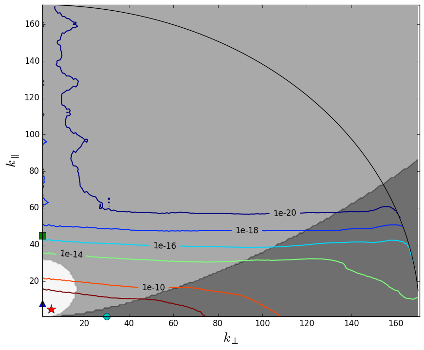
Figure 1: Contour levels of the energy spectrum as a function of parallel and perpendicular wave numbers, in the simulation of rotating turbulence with $\Omega=8$. Note the anisotropy of the spectrum, with most of the energy accumulating near modes with $k_{\parallel}\approx 0$. The white region corresponds to modes with $\tau_{\omega}<\tau_{s}<\tau_{NL}$ (i.e., modes dominated by the waves), the light grey region to modes with $\tau_{s}<\tau_{\omega}<\tau_{NL}$, and the dark grey region to modes with $\tau_{s}<\tau_{NL}<\tau_{\omega}$ (see text for details). Grey regions thus correspond to modes for which sweeping gives the fastest time scale (with dark grey indicating “slow” modes). The location of four modes relevant for the analysis are marked in the figure: the “wave” modes ${\bf k}=(0,0,8)$ (marked with a blue triangle) and ${\bf k}=(0,5,5)$ (marked with a red star), a “slow” (two-dimensional) mode in the dark grey region ${\bf k}=(0,30,0)$ (marked with a cyan circle), and the mode ${\bf k}=(0,0,45)$ in the light grey region (marked with a green square).

4.1 Numerical simulations

The code GHOST (Gómez et al., 2005; Mininni et al., 2011) is used to solve Eqs. (1) and (2) using a parallel pseudo-spectral method with a second order Runge-Kutta scheme for the time evolution. The $2/3$-rule is used for dealiasing. As will be seen below, computation of the contribution function requires high cadence I/O in time, and a significant amount of storage (note spatial information needs to be saved with twice the frequency of the fastest waves in the system). As a result, only simulations with moderate resolution can be performed. Here we present two simulations using grids of $N^{3}=512^{3}$ points in a three-dimensional periodic box.

Both simulations are identical except for the value of $\Omega$. In one of the simulations $\Omega=4$, while in the other $\Omega=8$. The simulations were started from the fluid at rest, and energy was injected via a mechanical forcing. We chose a Taylor-Green forcing of the form

$${\bf F} = F_{0}\left[\sin(k_{\textrm{TG},x}x)\cos(k_{\textrm{TG},y}y)\cos(k_{\textrm{TG},x}z)\hat{x}\right.$$ (22)

$$\left.-\cos(k_{\textrm{TG},x}x)\sin(k_{\textrm{TG},y}y)\cos(k_{\textrm{TG},z}z)\hat{y}\right],$$

with $F_{0}=0.277$, ${\bf k}_{\textrm{TG}}=(1,1,1)$ (which results in $L=2\pi/k_{\textrm{TG}}=2\pi/\sqrt{3}$), and $\nu=6.5\times 10^{-4}$ in dimensionless units (for unit velocity and a box of length $2\pi$). While other forcings will presumably produce similar results, Taylor-Green forcing was chosen because it has been reported to result in a larger amplitude of wave modes when compared with random-in-time isotropic forcing (Clark di Leoni et al., 2014). The system was let to reach a turbulent steady state with $U\approx 0.9$, which translates to a Reynolds number of approximately 5000, and a Rossby number of $0.03$ for $\Omega=4$ and of $0.015$ for $\Omega=8$. Once in t he turbulent steady state the simulations were allowed to run for over 12 large scale turn over times, the time span over which the following analysis was carried on.

4.2 Energy spectrum and decorrelation times

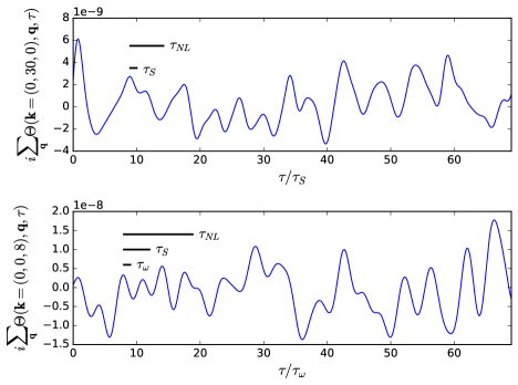
Figure 2: Partial reconstruction of $-{\partial\Gamma_{{\bf k}}}/{\partial\tau}$ via the sum over ${\bf q}$ of the third-order correlator $\Theta({\bf k},{\bf q},\tau)$, from Eq. (12) (computation of the real part by adding the complex conjugate is implied). The two panels show, from top to bottom, the results for ${\bf k}=(0,30,0)$ and for ${\bf k}=(0,0,8)$. The time lag $\tau$ is normalised by the dominant time scale ($\tau_{s}$ in the top panel, and $\tau_{\omega}$ in the bottom panel); the different timescales in these units are also shown as a reference by the horizontal bars in each figure. We recover the expected behaviour for the correlation functions, ${\bf k}=(0,0,8)$ (which is a fast mode) gets locked to the wave period, while ${\bf k}=(0,30,0)$ (which is slow) evolves in the sweeping time scale. The integral of these functions gives the correlation function, which decays rapidly on the dominant time scale.

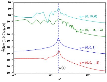
Figure 3: $|\widehat{\Theta}({\bf k}=(0,0,8),{\bf q},\omega)|$ as a function of $\omega$, for a fixed fast mode ${\bf k}$, and for different values of ${\bf q}$. Interactions with other wave modes (blue and red curves) show a well tuned spectrum centred around the wave frequency of the mode ${\bf k}$, indicating interactions are close to resonance. On the other hand, interactions with eddy modes (green and cyan curves) display a wider spectrum. All subsequent analyses of the contribution function focus on its maximum amplitude and on how well tuned each triad is (i.e., on the width of the peak around the maximum).

Before proceeding to the analysis of the contribution function, we first discuss some general properties of the simulations. In Fig. 1 we show contour levels of the axisymmetric energy spectrum for the simulation with $\Omega=8$, as a function of the perpendicular and parallel wave numbers (with the perpendicular and parallel directions defined with respect to the axis of rotation). Whilst in isotropic turbulence one would expect these contours to be circular, the effect of rotation in these flows impose a clear anisotropy, with a preferred accumulation of energy in modes with $k_{\parallel}\approx 0$ as predicted by Cambon & Jacquin (1989), Cambon et al. (1997), and Waleffe (1992). Moreover, a significant fraction of the energy is in modes with $k_{\parallel}=0$, for which resonant interactions cannot account for.

Three different regions are shaded in Fig. 1. The white region corresponds to modes with $\tau_{\omega}<\tau_{s}<\tau_{NL}$. This is the region of “fast” (or “wave”) modes, for which the period of the waves is the fastest time scale. The grey region corresponds to modes with $\tau_{s}<\tau_{\omega}<\tau_{NL}$. Although these modes are often considered to be “fast”, as shown in Clark di Leoni et al. (2014) these modes are decorrelated in a timescale which is of the order of the sweeping time. In other words, in the Eulerian frame, the dominant time scale for these modes is given by the sweeping, which is the shortest available time. Finally, in the dark grey region the modes have $\tau_{s}<\tau_{NL}<\tau_{\omega}$. This is the region of “slow” modes for which the eddies are faster than the waves. The three shaded regions are shown only as a reference. To compute the value of $\tau_{NL}$ at each wave number using Eq. (7), an estimation of $E(k)$ is needed. For simplicity, instead of using the measured spectrum, we use the phenomenological expression for non-helical rotating turbulence $E(k)\sim\epsilon^{1/2}\Omega^{1/2}k^{-2}$ (Zhou, 1995; Müller & Thiele, 2007; Mininni et al., 2012). In Clark di Leoni et al. (2014) it was shown, from direct computation of the decorrelation times, that this choice results in a good estimation of the dominant time scale for modes laying in the inertial range (i.e., at small and intermediate wave numbers). At large wavenumbers, where the spectrum drops exponentially as a result of viscous damping, $\tau_{NL}$ departs from this estimation. However, we will not consider modes in the viscous range, for which also the viscous damping time can be relevant.

The ordering of the time scales described above has implications for the behaviour of the time correlation function $\Gamma_{\bf k}(\tau)$. In the white region of Fig. 1, $\Gamma_{\bf k}(\tau)$ is expected to decay to $1/e$ of its value for $\tau=0$ in one wave period of the mode with wave vector ${\bf k}$ (Favier et al., 2010; Clark di Leoni et al., 2014). This time scale is what we define as the decorrelation time: after this time, the mode ${\bf k}$ has significantly decorrelated from its previous state. As already mentioned, in the two grey regions the function $\Gamma_{\bf k}(\tau)$ decays to $1/e$ of its value for $\tau=0$ in a time equal to $\tau_{s}$ (Clark di Leoni et al., 2014). We will thus consider modes in these three regions to compute the third order correlators $\Theta({\bf k},{\bf p},{\bf q},\tau)$ and $\hat{\Theta}({\bf k},{\bf p},{\bf q},\omega)$. In particular, in Fig. 1 we indicate two fast modes ${\bf k}=(0,5,5)$ and $(0,0,8)$, a “swept” mode $(0,0,45)$, and a slow mode $(0,30,0)$. These modes will be used in several examples below.

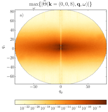
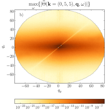
Figure 4: Intensity (as a function of ${\bf q}$) of the maximum of the contribution function, $\max_{\omega}\{|\widehat{\Theta}({\bf k},{\bf q},\omega)|\}$. In each panel, ${\bf k}$ is fixed, and the maximum of $|\widehat{\Theta}|$ is plotted for all available triads by varying ${\bf q}$. Two ${\bf k}$ modes are considered, a) ${\bf k}=(0,0,8)$ and b) $(0,5,5)$, both dominated by waves. The black dots in the centre indicate the modes ${\bf q}=\pm{\bf k}$. Two prominent features arise. One is the effect of the anisotropy of the flow, as triads with larger amplitudes are distributed along horizontal bands (i.e., coupling the ${\bf k}$ modes with modes with smaller vertical wave numbers). The other is the defect along the line ${\bf q}=\alpha{\bf k}$, as collinear modes do not contribute to the triads in an incompressible fluid.

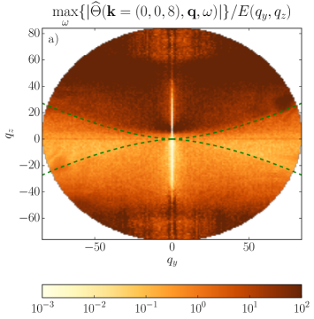
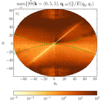
Figure 5: Intensity of the peak values of the normalised contribution function for each triad, given by $\max_{\omega}\{|\widehat{\Theta}({\bf k},{\bf q},\omega)|\}/E(q_{y},q_{z})$. In each panel, ${\bf k}$ is fixed for two modes dominated by waves: a) ${\bf k}=(0,0,8)$, and b) ${\bf k}=(0,5,5)$. The dashed lines represent the modes with $\tau_{\omega}=\tau_{NL}$. Modes with $\tau_{\omega}<\tau_{NL}$ (those above the upper dashed line) have higher frequencies (i.e., shorter time scales), and are thus preferred. Note however there is a non-negligible leakage towards slow modes ${\bf q}$ with $\tau_{\omega}\gtrsim\tau_{NL}$ (i.e., modes slightly below the dashed upper curve).

4.3 Analysis of third-order time correlators

Equation (12) indicates that the nonlinear interaction with all triads gives rise to the time decorrelation of the mode at a given ${\bf k}$. In other words, the apparently random contribution of all nonlinear triads results in the deformation of the structure to the point that the mode decorrelates with itself, and thus transfers its energy to other modes in the allowed triads. As a result, $\Gamma_{\bf k}(\tau)$ decreases for short increments $\tau$, and then fluctuates around zero. $-\partial\Gamma_{\bf k}(\tau)/\partial\tau$ should then start from zero for $\tau=0$, increase to a maximum, and then fluctuate with the dominant time scale of the mode. Figure 2 shows a partial reconstruction of $-{\partial\Gamma_{{\bf k}}}/{\partial\tau}$ by computing a partial sum over ${\bf q}$ of the $\Theta({\bf k},{\bf q},\tau)$ function for ${\bf k}=(0,0,8)$ and for ${\bf k}=(0,30,0)$. The partial reconstruction is done using Eqs. (12) and (16), i.e., we sum $\Theta$ over the subset of ${\bf p}$ and ${\bf q}$ modes available for the analysis and that satisfy the relation ${\bf p}+{\bf q}={\bf k}$. Due to the large amount of data required for this computation, we only consider modes in the $(k_{x}=0,k_{y},k_{z})$ plane, and therefore we only sum over the triads with ${\bf p}\cdot\hat{x}={\bf q}\cdot\hat{x}=0$, resulting in the partial reconstruction mentioned above. Nonetheless, this suffices to get the expected behaviour for the time derivative of the decorrelation functions. For the mode ${\bf k}=(0,0,8)$, which is a fast mode, the time derivative gets locked to the wave period, while for ${\bf k}=(0,30,0)$, which is a slow mode, the dominant time scale is the sweeping time. Here and in the following, except when duly noted, all results shown are for the $\Omega=8$ simulation.

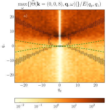
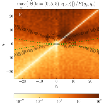
Figure 6: Close up of the geometric distribution of the peak value of the normalised contribution function for each triad, given by $\max_{\omega}\{|\widehat{\Theta}({\bf k},{\bf q},\omega)|\}/E(q_{y},q_{z})$. As in Fig. 5, in each panel ${\bf k}$ is fixed to consider two modes dominated by waves: a) ${\bf k}=(0,0,8)$, and b) ${\bf k}=(0,5,5)$. The dashed curves represent the modes with $\tau_{\omega}=\tau_{NL}$, and the circles represent the near-resonant modes (according to the theoretical prediction) with $\gamma_{r}<0.1$. In good agreement with wave turbulence theories, normalised resonant triads have large amplitudes, but some near-resonant triads are also strong. In panel ${\it b)}$, some of these near-resonant triads have non-negligible coupling with slow modes (see the circles near $q_{y}\approx 10$ and $q_{z}\approx 0$) allowing for energy transfer towards these modes.

4.4 Contribution functions

We now present our analysis of the behaviour of the contribution function $\Theta$. Figure 3 shows the value of $|\widehat{\Theta}({\bf k}=(0,0,8),{\bf q},\omega)|$ as a function of $\omega$, for four different values of ${\bf q}$ (i.e., for four different triads). All of them peak at $\omega_{0}=\omega({\bf k})$, which is the wave frequency of the mode ${\bf k}$. This was checked for other values of ${\bf k}$ as well, and a peak in the corresponding wave frequency was observed in all cases except for the modes with $k_{\parallel}\approx 0$ (i.e., the slow modes), for which no discernible peak is present. Moreover, and in spite of the presence of a peak for modes with $k_{\parallel}>0$, it is worth noting that the width of the peak depends strongly on the nature of the other modes in the triad. While interactions with other wave modes have most of the power in the peak and are well tuned (i.e., the peak is relatively narrow), interactions with slow modes can have large amplitudes but with a broad spectrum.

This gives a direct way to identify not only the strength of a given triad, but also to measure how resonant the triad is, as more resonant triads are expected to result in a sharper spectrum of $\widehat{\Theta}({\bf k},{\bf q},\omega)$ per virtue of Eq. (20). Therefore, to simplify the analysis, we can focus on a few modes ${\bf k}$, explore all available values of ${\bf q}$ on a triad with ${\bf k}$, and look only at the the maximum value of $\widehat{\Theta}$ (for all $\omega$) and on the relative width of the maximum (i.e., on how well tuned the interaction is around $\omega_{0}$).

In Fig. 4 we show $\max_{\omega}\{|\widehat{\Theta}({\bf k},{\bf q},\omega)|\}$ for two modes ${\bf k}=(0,0,8)$ and $(0,5,5)$, as a function of all possible values of ${\bf q}$ in the $(0,q_{y},q_{z})$ plane. The anisotropic nature of rotating turbulence makes a stellar apparition here, as the distribution of values is clearly influenced by it. The result indicates that triads which are elongated along the horizontal direction have larger amplitudes, which is compatible with the prediction that energy tends to go towards the slow modes (with $q_{z}\approx 0$) as discussed in Waleffe (1992). Indeed, the triads with larger amplitudes are located in a horizontal band within $-k_{z}\lesssim q_{z}\lesssim k_{z}$. There are also strong triads that couple the ${\bf k}$ mode with modes with larger vertical wavenumber (i.e., triads in the horizontal bands $k_{z}\lesssim|q_{z}|\lesssim 2k_{z}$) which are compatible with an anisotropic transfer of a fraction of the energy towards larger wave numbers (i.e., smaller scales). Finally, collinear modes (i.e., modes with ${\bf q}=\alpha{\bf k}$) make no contribution to the triads as a result of the incompressibility of the fluid.

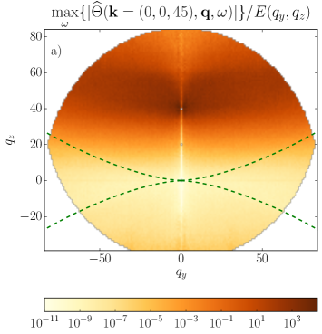
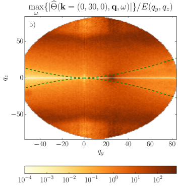
Figure 7: Peak values of the normalised contribution function for each triad, given by $\max_{\omega}\{|\widehat{\Theta}({\bf k},{\bf q},\omega)|\}/E(q_{y},q_{z})$. The panels correspond to two fixed values of ${\bf k}$: a) a small-scale “fast” mode ${\bf k}=(0,0,45)$, and b) a small-scale “slow” mode ${\bf k}=(0,30,0)$. The dashed curves represent the modes with $\tau_{\omega}=\tau_{NL}$. The role played by resonant and near-resonant interactions in these cases is less clear.

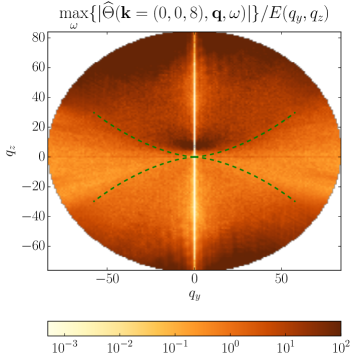
Figure 8: Peak values of the normalised contribution function for each triad, $\max_{\omega}\{|\widehat{\Theta}({\bf k}=(0,0,8),{\bf q},\omega)|\}/E(q_{y},q_{z})$, for the simulation with weaker rotation (i.e., larger Rossby number). Results are similar to the case with stronger rotation, although the contrast in intensity between triads involving fast and slow waves is less clear.

4.5 Normalised contribution functions

Having said this, it can be argued that the strongest triads correspond to modes with $q_{z}\approx 0$ only as a result of the anisotropic energy spectrum shown in Fig. 1: the modes with small vertical wavenumber have most of the energy, and as a result triads involving those modes will have larger amplitudes. Therefor, we can normalise the triads by the energy of the q mode in the triad, i.e., we can compute $\max_{\omega}\{|\hat{\Theta}({\bf k},{\bf q},\omega)|\}/E({\bf q}).$ If this is done, from Eqs. (12) and (19) the normalised contribution function has units of inverse time (i.e., of frequency). This time can thus be interpreted as the time scale of the energy transfer mechanism, as it is often done in turbulence theories.

We now turn to the analysis of these normalised contribution functions. In Fig. 5 we show the peak value of the normalised functions for ${\bf k}=(0,0,8)$ and $(0,5,5)$. Two dashed curves indicate the modes for which $\tau_{\omega}=\tau_{NL}$, i.e., modes with the eddy turnover time equal to the period of the waves. Modes respectively above and below the upper and lower curves have $\tau_{\omega}<\tau_{NL}$, and are dominated by the waves. Modes between the two dashed curves have $\tau_{\omega}>\tau_{NL}$, and are slow modes dominated by the eddies.

Anisotropic effects are still evident in Fig. 5 after the normalisation, but the role played in the triads by the waves starts to become more clear. Although wave modes have less energy, after normalisation it becomes evident that triadic interactions of the wave modes ${\bf k}=(0,0,8)$ and $(0,5,5)$ with other wave modes are relatively stronger than interactions with slow modes. If the normalised contribution function is interpreted as an inverse transfer time, it then implies that the transfer between triads involving waves is faster than triads involving slow modes, and thus should be preferred for the interaction. This is true even for modes ${\bf q}$ with $\tau_{s}<\tau_{\omega}<\tau_{NL}$, i.e., for modes with sweeping time faster than the wave period (but with the waves still dominating over the eddies).

Large amplitudes (or, equivalently, shorter transfer times) can be seen in Fig. 5 in the vicinity of ${\bf q}\approx{\bf k}$. Although at first glance it would appear that this is due to local (in Fourier space) interactions being the most prominent, closer inspection reveals that it is also due to the effect of resonances. In Fig. 6 we show a close up of the normalised contribution functions in Fig. 5 for small values of $|{\bf q}|$. Circles mark the modes that satisfy the theoretical near-resonant condition up to a value of $\gamma_{r}=0.1$. It is evident that many of the strongest triads correspond to resonant or near-resonant triads. This is in very good agreement with wave turbulence theories of rotating turbulence, which predict that resonant triads should dominate the coupling between modes (Newell, 1969). However, this also explains how the system transfers energy towards slow modes, which are inaccessible in weak wave turbulence approximations. The data in Fig. 6 indicates that not only resonant triads are relevant, but that near-resonant triads play an equally important role (at least for the case of a periodic flow). Indeed, large amplitudes can be seen around the circles in Fig. 6 in a region that is even broader than the fan corresponding to the condition $\gamma_{r}=0.1$. Close observation of Fig. 6 a) and b) (as well as the observation of other modes ${\bf k}$ not shown here) gives rise to the following picture: For ${\bf k}=(0,0,8)$, resonant and near-resonant interactions couple this mode with some modes with $q_{z}/q<k_{z}/k$, thus allowing an energy exchange between these modes. Energy can thus be transferred towards modes with smaller vertical wavenumber, in agreement with the arguments in Cambon & Jacquin (1989) and Waleffe (1993). For ${\bf k}=(0,5,5)$, the process is repeated, but now some near-resonant interactions allow for a coupling (and thus a transfer) with slow modes. This is compatible with observations in Smith & Lee (2005), Alexakis (2015), and Gallet (2015). Moreover, in Fig. 6 b) a non-negligible coupling with slow modes can be observed even for non-resonant triads (see the region between the two-dashed curves with $q_{y}>0$), indicating that as energy approaches the slow modes the role of non-resonant interactions may also become more relevant.

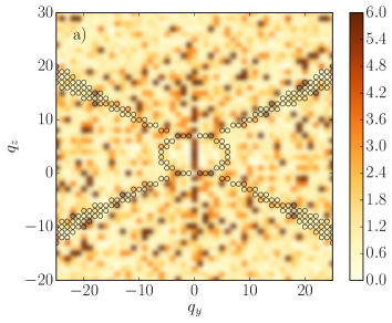
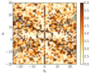
Figure 9: Inverse relative bandwidth (quality factor) of the peak in each contribution function, as a function of ${\bf q}$, and for fixed ${\bf k}=(0,0,8)$, a) for the simulation with $Ro\approx 0.03$, and b) for the simulation with $Ro\approx 0.015$. Larger quality factors correspond to sharper bandwidths of the triads relative to their central frequency, and thus to more resonant interactions (i.e., the factor quantifies how well tuned a triad is). Circles indicate modes which satisfy the theoretical near-resonance condition with $\gamma_{r}<0.1$. A good agreement is observed between the theoretical condition and the quality factor of the contribution function, specially for the flow with smaller Rossby number. Note however that relatively large quality factors are observed for branches which are wider than the condition $\gamma_{r}<0.1$, indicating again the important role played by near-resonant interactions.

4.6 Comparison with small-scale and slow modes

To gain more certainty on the effect of the waves in the triadic interactions, we compare now the previous results with the normalised contribution function for two modes: a small-scale mode with ${\bf k}=(0,0,45)$, which is dominated by sweeping (but with the wave period faster than the eddy turnover time), and a small-scale slow mode with ${\bf k}=(0,30,0)$ which has zero wave frequency. Here, by small-scale, we refer to modes with wave numbers significantly larger than the forced wave number. The resulting normalised contribution functions are shown in Fig. 7. In both cases, the division given by the curve with $\tau_{\omega}=\tau_{NL}$ is less evident, and a superposition of the modes expected to be resonant or near-resonant (not shown) indicates no clear correlation between the strength of the triad and the theoretical resonant or near-resonant condition. For the mode ${\bf k}=(0,0,45)$, the normalised contribution function indicates that coupling is stronger for modes with $q_{z}\approx k_{z}$, an effect associated with the anisotropy of the flow, while the coupling with slow modes is negligible. The slow mode ${\bf k}=(0,0,45)$ shows more interesting features. The mode seems to be more strongly coupled with other slow modes ${\bf q}$ in the vicinity of ${\bf k}$, and with modes with large $q_{z}$ (of the order of $|{\bf k}|$, compatible with local triadic interactions, although these interactions are non-resonant).

4.7 Effect of the Rossby number

We can also compare the results in the two simulations with different Rossby number, to quantify the effect of changing the rotation frequency in the intensity of resonant and near-resonant triads. As an illustration, Fig. 8 shows the geometric distribution of the peak values of the normalised contribution function for the mode ${\bf k}=(0,0,8)$ in the simulation with larger Rossby number. The same result as in Fig. 5 is obtained, but the contrast between modes above and below the $\tau_{\omega}=\tau_{NL}$ curve is less marked. Also, the region of modes dominated by eddies (i.e., of slow modes) increases as expected, and the boundary between the two regions indicated by the change in intensity of the triads moves accordingly. This confirms that the changes in intensity in Fig. 5 indeed separate triads involving slow and fast modes, and is also consistent with the behaviour expected in a rotating flow as the Rossby number is varied.

4.8 Direct measurement of the resonance level of each triad

One of the most important implications of the contribution function is that it allows a direct measurement of how well tuned a triad is, i.e., of how resonant the interaction between three modes is. This was already discussed in the context of Fig. 3, where we showed that some triads display a narrower peak around the wave frequency than others. But now we can put this observation on firmer grounds.

As it follows from Eq. (20), for a perfectly resonant triad the contribution function should be a delta distribution centred around $\omega_{0}=\omega({\bf k})$. Near-resonant and non-resonant interactions broaden the peak. This broadening can be measured using the quality factor

$$Q=\frac{\omega_{0}}{\Delta\omega}.$$ (23)

In other words, the $Q$ factor is the inverse relative width of the peak of $\widehat{\Theta}({\bf k},{\bf q},\omega)$ as a function of the frequency. We estimate $\Delta\omega$ by calculating the width of the peak in the spectrum (see Fig. 3) at half the amplitude of the maximum value. In the theory of resonators, the $Q$ factor is often interpreted as the ratio of the energy stored to the energy lost in a system. In our case, the larger the $Q$ factor the more resonant the triad is, and the less energy of the mode ${\bf k}$ is lost (i.e., given) to non-resonant modes.

Figure 9 shows this quality factor for each contribution function for fixed ${\bf k}=(0,0,8)$ and for all possible values of ${\bf q}=(0,q_{y},q_{z})$, for the two simulations with different Rossby numbers. Superimposed to the quality factor, circles mark the modes that satisfy the theoretical near-resonant condition up to a value of $\gamma_{r}=0.1$. In particular for the simulation with smaller Rossby number, triads with large quality factors (i.e., well tuned triads) more or less coincide with triads with small $\gamma_{r}$, specially for the branches in the upper-left and lower-right quadrants on the figure on the right in Fig. 9. In other words, the quality factor defined above gives a good measure of how resonant a triad is. Moreover, three features in Fig. 9 are worth emphasising: First, the $Q$ factor has maximum values $\approx 6$ which is of the order of, although a bit smaller than, what is often found in electrical or mechanical resonators. In other words, even resonant triads display broadband peaks in the frequency spectrum. Second, the area covered by triads with the largest values of $Q$ is relatively larger than the area corresponding to the circles with $\gamma_{r}<0.1$, confirming the importance of interactions that are even marginally near-resonant. The scaling of this behaviour with Rossby number and domain size can be important for theories of rotating turbulence in infinite domains, in which the behavior of the resonant and slow manifolds, as well as the relevance of near-resonances, are unclear (Cambon et al., 2004; Chen et al., 2005; Bourouiba, 2008). Third, there are some modes with relatively large $Q$ values (compared with the mean amplitude of $Q$ for all modes) that do not correspond to resonant or near-resonant modes in wave turbulence theory. Most notably, some of these modes are modes with small $|{\bf q}|$ and lying in the region of the slow modes.

5 Conclusions

One of the central problems in turbulence theory involves the understanding of how modes interact non-linearly, specially in systems with restitutive forces for which eddies and waves can coexist, and for which resonances can strongly affect the nonlinear triadic interactions. In these problems, a direct investigation of how each triad of modes contributes to the overall dynamics is quite cumbersome and complicated. To tackle this problem we have derived a contribution function that characterises the spatio-temporal behaviour of each triad, and more importantly, their contribution to the energy transfer and to the spatio-temporal spectrum of the turbulent flow.

We used this function to study the case of rotating turbulence, in which eddies coexist with inertial waves, and where triadic resonant interactions are expected to be dominant (Newell, 1969), transferring their energy preferentially towards modes with small vertical wave numbers (Cambon & Jacquin, 1989; Waleffe, 1993). However, this picture fails to explain how energy continues to be transferred anisotropically to “slow” two-dimensional modes, as the wave turbulence approximation breaks down in the vicinity of those modes. Previous results in simulations at low resolution or in truncated systems (Chen et al., 2005; Smith & Lee, 2005) indicate that near-resonant triads can be responsible for this latter transfer, but it is still unclear whether these interactions remain to be relevant as the turbulence level is increased, or as the Rossby number is decreased. Some recent results suggest this to be the case (Alexakis, 2015; Gallet, 2015).

We computed the contribution function for a large number of triads in two simulations of rotating turbulence at spatial resolutions of $512^{3}$ grid points. As the contribution function is a third-order time-correlation function for each Fourier triad, this requires a massive analysis of spatio-temporal data. The main results show or confirm that: (1) For “wave” modes with $\tau_{\omega}<\tau_{s}<\tau_{NL}$ (i.e., modes for which the wave period is faster than the sweeping time and the eddy turnover time), the coupling between triads is strongly anisotropic. Triads which are elongated along the horizontal direction have larger amplitudes, a result which is compatible with the prediction that energy tends to go towards modes with smaller parallel wave numbers. This result is also in agreement with the proposed mechanism of parametric instability, which was obtained for isolated triads (Waleffe, 1993), while the data analysis presented here considers the system with all possible couplings between the triads. (2) After normalising the triads by the energy in one of modes, it is found that the transfer between triads involving wave modes is faster than the transfer between triads that couple the wave mode with a slow mode, and thus the former can be expected to be the preferred ones for interactions, also in agreement with predictions from wave turbulence theory. (3) However, near-resonant and non-resonant interactions are non-negligible, and couple the wave modes to slow modes, thus allowing for energy transfer into that region of spectral space. (4) The contribution function is peaked around the frequency of each mode, and thus can be used to define a quality factor $Q$ that measures how resonant a triad is. While resonant triads are compatible with relatively larger values of the $Q$ factor, the analysis shows that some marginally near-resonant and non-resonant triads also display tuning with the wave frequency and are such that can couple fast and slow modes. Further studies of this result can be importat for theories of rotating turbulence in infinite domains, in which the nature and coupling of the modes in the slow and in the resonant manifolds with the rest of the modes is a matter of debate. (6) For modes for which $\tau_{\omega}$ is larger than $\tau_{s}$ or $\tau_{NL}$, the relevance of resonant and near-resonant triads decreases rapidly. (7) Finally, varying the Rossby number qualitatively preserves these results, at least in the short range of values considered here.

These results are in agreement with major theoretical predictions for the behaviour of nonlinear interactions in rotating turbulence, as mentioned above, and can shed some light on the recent results concerning the behaviour or two-dimensional modes for very small Rossby numbers. In this context, an obvious shortcoming of the present study is the lack of a parametric study of the behaviour of the triads for even smaller Rossby numbers, or for larger Reynolds numbers. The need to properly resolve in time the fastest waves and to store with high time cadence the data, to then perform the spatio-temporal analysis of each triad, precludes for the moment studies with faster rotation or with larger spatial resolution. However, we believe that the results presented here can be useful to quantitatively assess the relevance of resonant, near-resonant, and non-resonant triads at moderate Rossby numbers. Also, the formalism presented here can be extended to analyse other systems in which resonant interactions are also believed to play a central role (see, e.g., the recent studies by Aubourg & Mordant (2015, 2016)).