Stochastic Search with Poisson and Deterministic Resetting

Abstract

We investigate a stochastic search process in one, two, and three dimensions in which $N$ diffusing searchers that all start at $x_{0}$ seek a target at the origin. Each of the searchers is also reset to its starting point, either with rate $r$, or deterministically, with a reset time $T$. In one dimension and for a small number of searchers, the search time and the search cost are minimized at a non-zero optimal reset rate (or time), while for sufficiently large $N$, resetting always hinders the search. In general, a single searcher leads to the minimum search cost in one, two, and three dimensions. When the resetting is deterministic, several unexpected feature arise for $N$ searchers, including the search time being independent of $T$ for $1/T\to 0$ and the search cost being independent of $N$ over a suitable range of $N$. Moreover, deterministic resetting typically leads to a lower search cost than in stochastic resetting.

1 Introduction

Stochastic searching [1] underlies many biological processes [2, 3, 4], animal foraging [5, 6, 7, 8, 9], as well as operations to find missing persons or lost items [10, 11, 12]. In these settings basic goals are to maximize the probability that the target is actually found and to minimize the time and/or the cost required to find the target. In response to these challenges, a wide variety of search algorithms have been extensively investigated and rich dynamical behaviors have been uncovered [14, 15].

Typically, one or perhaps multiple searchers move in some fashion through a search domain to locate either a single target or a series of targets. The most naive setting is that of a single searcher has no information about the target and moves by random-walk, or equivalently, diffusive motion. Such a search is generally hopelessly inefficient because the target may not be found, for spatial dimension $d\geq 3$, or the average search time is infinite. Thus much effort has been directed to uncover more effective search strategies

Many such possibilities have been investigated. One natural mechanism is to allow the searcher to move according to a Lévy flight (see, e.g., [8, 16, 13]), so that the search can quickly cover large distances between targets. A somewhat related example is that of intermittent search, in which the search process is partitioned into periods of intensive search, during which the searcher moves slowly, and superficial search, during which the searcher moves quickly [17]. In the context of searching for nourishment, the essential tradeoff is how long to continue to exploit resources in a local area and when to move to a new area as local resources become depleted [5, 18, 19]. These notions also underlie the search for a target along a DNA by a diffusing protein [2, 3, 20, 21, 22, 23], where the tradeoff is for the search to diffuse along the DNA or unbind and reattach at some distant point along the DNA.

Very recently, the mechanism of search that is augmented by “resetting” was introduced [24, 25, 26]. In this model, a target is placed at the origin (without loss of generality) and a searcher starts at some arbitrary point. In addition, the searcher returns to a fixed “home base” at a given rate during the search. If the distance between the home base and the target is known with certainty, then a search based on a stochastically moving searcher is not a pertinent approach. However, the natural situation is that the target location is only partially known; for example, the target is somewhere within a finite body of water. In this case, a relevant parameter is the maximum possible distance between the target and the home base. As shown in [26], the basic properties of search with resetting when the distance between the target and home base is known precisely are qualitatively the same as the situation where only the probability distribution of this distance is known. Thus for the purposes of tractability we restrict ourselves to the idealized (and admittedly unrealistic) situation where the distance between the target and home base is known.

In general, resetting is known to have a dramatic effect on the search. A diffusing particle requires an infinite average time to reach a target in spatial dimensions $d=1$ and $d=2$, and the searcher may not even reach a finite-size target for $d>2$. However, resetting ensures that: (i) the searcher can always find the target in any dimension and (ii) the average search time is finite. Overall, therefore, resetting gives rise to a more efficient search. One of the basic results of recent investigations of search with resetting [24, 25, 26] was to determine the conditions that optimize the search time. This resetting mechanism has also been quite fruitful conceptually and a variety of interesting consequences of resetting have been elucidated [27, 28, 29, 30, 31, 32, 33, 34, 35, 36].

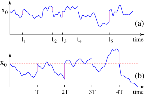
Figure 1: Contrast of the trajectories in: (a) Poisson reset and (b) deterministic reset with reset time $T$. The target is at the origin and the reset point is $x_{0}$.

In this work, we investigate two as yet unexplored features of search with resetting: (i) $N$ searchers, each of which is reset at the same Poisson rate, to a “home base”, and (ii) deterministic reset, in which the searchers return to the home base after a fixed operation time, rather than the searchers being reset according to a fixed-rate Poisson process (Fig. 1). The related situation of many searchers that are uniformly distributed in space, each of which is reset to its own starting position at a fixed rate, was investigated in [26]. However, in the context of search for a missing person, it is natural that all the searchers return to a single home base (or perhaps a small number of such bases). Moreover, in such a search, activities are typically suspended at the end of daylight or when searchers reach their physical limits. Thus it is also realistic to investigate the situation in which all the searchers are reset to a given location at a fixed reset time.

In the next section, we start by briefly reviewing known results about stochastic search by a single searcher in one dimension ($d=1$), with the additional feature that the searcher is reset to its home base at a fixed rate. We will also present our renewal-based approach to solve this problem that will be employed throughout this work. Next, we treat the case of $N$ searchers in one dimension, each of which is independently reset to the same location at a fixed rate $r$. We show that for $N<N^{*}$ there is an optimal non-zero reset rate $r^{*}_{N}$ that minimizes the search time as well as the search cost, while for $N>N^{*}$ resetting always hinders the search. We also determine this critical number $N^{*}$ analytically. In Sec. 3, we turn to search with stochastic resetting in spatial dimensions $d=2$ and $d=3$. For the case of $d=3$, we exploit a well-known construction to reduce the diffusion equation in three dimensions to an effective diffusion equation in one dimension. This allows us to obtain results about three-dimensional search in terms of the corresponding one-dimensional system.

To probe the properties of the $N$-searcher system in a convincing way, we outline, in Sec. 4, an efficient event-driven simulation in one dimension that obviates the need to microscopically follow the trajectories of each searcher between reset events. By exploiting the aforementioned dimensional reduction of the three-dimensional diffusion equation, we can also directly adapt our event-driven approach to three dimensions. For $d=2$, no such dimensional reduction exists and our simulations are based on a more direct approach. From these numerical approaches, we determine the condition for optimal search for both a single searcher and for many searchers in spatial dimensions $d=1$ and 3, and then $d=2$.

Finally, in Sec. 5, we investigate the case of deterministic resetting, for both a single and for many searchers, again for the cases of $d=1$, $d=3$, and then $d=2$. The salient feature of deterministic resetting is that it leads to a quicker search than stochastic resetting at their respective optimal resetting rates (or times). Moreover, deterministic resetting leads to a search cost that, for large $N$, is nearly independent of the reset rate $r$ over a wide range of $r$. Concluding remarks are given in Sec. 6.

2 Poisson Resetting in One Dimension

As mentioned above, the situation where a searcher is reset at a fixed rate $r$ has already been extensively investigated [24, 25, 26]. For completeness, we quote the main results for this type of search and also derive them by an independent method. We then investigate the case of $N$ independent searchers, each of which is reset to a common point at the same rate $r$.

2.1 One searcher

Consider a target that is fixed at the origin and a diffusing searcher that is reset to a point $x_{0}$ at rate $r$. For simplicity, we assume that the searcher begins at this reset point. For this system, the first two moments of the search time are (see Refs. [24, 25] and also A)

$$\begin{split}\langle t_{1}\rangle&=\frac{1}{r}\left(e^{x_{0}\sqrt{{r}/{D}}}-1\right)\,,\\ \langle t_{1}^{2}\rangle&=\frac{1}{r^{2}}\left[e^{x_{0}\sqrt{{r}/{D}}}\big{(}2\,e^{x_{0}\sqrt{{r}/{D}}}-x_{0}\sqrt{{r}/{D}}-2\big{)}\right]\,,\end{split}$$ (1)

and higher moments can be extracted straightforwardly. The subscript 1 signifies one searcher. The basic feature of (1) is that $\langle t_{1}\rangle$ is minimized at an optimal reset rate $r^{*}$ that is of the order of $D/x_{0}^{2}$. The inverse of the optimal rate gives the typical time between resets as roughly $T_{D}\equiv x_{0}^{2}/D$, the time for a diffusing particle to reach a distance $x_{0}$. If the searcher does not find the target within this time, then it is likely wandering in the wrong direction and will reach the target at a time much greater than $T_{D}$. In this case, it is better to reset this errant searcher back to its home base than allowing it to continue on its current trajectory.

We now give an independent derivation for the average search time $\langle t_{1}\rangle$ that relies on the renewal nature of the search process; a similar approach was very recently developed in Ref. [38]. Namely, whenever a reset occurs, the process restarts at the initial condition, but with the proviso that the time is incremented appropriately to account for the return to the reset point. As a preliminary, we need the following:

$$R(t) \equiv\text{prob.\ reset time is greater than}\ t\,,$$

$$S(x_{0},t) \equiv\text{prob.\ hitting time is greater than}\ t\,.$$

For diffusive motion, $S(x_{0},t)$ is also the “survival probability” that a searcher initially at $x_{0}$ has not reached the origin by time $t$ is [39]

$$S(x_{0},t)=\text{erf}\Big{(}\frac{x_{0}}{\sqrt{4Dt}}\Big{)}\,.$$ (2a)

Correspondingly, the first-passage probability that a diffusing particle initially at $$x_{0} t$$ first reaches the origin at time is

$$F(x_{0},t)=-\frac{dS(x_{0},t)}{dt}=\frac{x_{0}}{\sqrt{4\pi Dt^{3}}}\,\,e^{-x_{0}^{2}/4Dt}\,\,.$$ (2b)

Since the search process is specified by whether the target is reached before a reset occurs and vice versa, we also define two fundamental probabilities:

$$\begin{split}P&\equiv\text{prob.\ target hit before reset}=\int_{0}^{\infty}\!\!dt\underbrace{~{}\left(-\frac{dS(x_{0},t)}{dt}\right)~{}}_{\text{prob.\ hit in $(t,t+dt)$}}\times\ \underbrace{~{}~{}~{}R(t)~{}~{}~{}}_{\text{prob.\ reset time $>t$}}\!\!\!\!\!,\\ Q&\equiv\text{prob.\ reset before target hit}=\int_{0}^{\infty}\!\!dt\underbrace{~{}~{}S(x_{0},t)~{}~{}}_{\text{prob.\ hit time $>t$}}\,\times\,\underbrace{~{}~{}\left(-\frac{dR(t)}{dt}\right)~{}~{}}_{\text{prob.\ reset in $(t,t\!+\!dt)$}}\!\!\!\!.\end{split}$$ (3)

Thus the “direct” time for the target to be reached before a reset occurs, which we define as $t_{d}$, is

$$t_{d}=\int_{0}^{\infty}\!\!dt\,t\,\left(-\frac{dS(x_{0},t)}{dt}\right)\,\times\,R(t)\Big{/}P\,.$$ (4a)

Similarly, the “reset” time $$t_{r}$$ for a reset to occur before the target is reached is

$$t_{r}=\int_{0}^{\infty}\!\!dt\,t\,\left(-\frac{dR(t)}{dt}\right)\,\times\,S(x_{0},t)\Big{/}Q\,.$$ (4b)

Using the renewal nature of the search, $\langle t_{1}\rangle$ satisfies the recursion

$$\langle t_{1}\rangle=Pt_{d}+Q\big{(}t_{r}+\langle t_{1}\rangle\big{)}\,.$$ (5a)

The first term accounts for hitting the target before a reset occurs, while the second term accounts for the search restarting after a reset. In this latter case, the search is delayed by $$T_{r} T_{d}=P\,t_{d} T_{r}=Q\,t_{r} \langle t_{1}\rangle$$. For notational convenience, we define and . Solving for gives

$$\langle t_{1}\rangle=\frac{T_{d}+T_{r}}{1-Q}\,\,.$$ (5b)

This result is general and can be applied to higher dimensions and to different reset mechanisms, as will be discussed later.

Since only the sum $T_{d}+T_{r}$ appears in the expression for $\langle t_{1}\rangle$, we add the two lines in (4a) and integrate by parts to give

$$T_{d}+T_{r}=\int_{0}^{\infty}dt\,R(t)\,S(x_{0},t)\,.$$ (6)

We now specialize to Poisson resetting with rate $r$, for which $R(t)=e^{-rt}$. Using this, as well as (2a) for $S(x_{0},t)$, the integrals in (3) and (6) are

$$T_{d}+T_{r} =\frac{1}{r}\!\left(1\!-\!e^{-x_{0}\sqrt{r/D}}\right)\,,$$

$$Q =1-e^{-x_{0}\sqrt{r/D}}\,.$$

from which (5b) gives

$$\langle t_{1}\rangle=\frac{1}{r}\left(e^{x_{0}\,\sqrt{r/D}}-1\right)\,.$$ (7)

This reproduces Eq. (1) as it must.

2.2 Multiple searchers

Since all searchers are independent and the target location is fixed, it is theoretically possible to obtain the survival probability of the target in the presence of $N$ searchers as the $N^{\rm th}$ power of the target survival probability due to a single searcher. However, while the Laplace transform of the target survival probability with one searcher is known exactly, Eq. (26), it does not appear possible to Laplace invert this expression exactly. Nevertheless, we can invert this Laplace transform in the limit $r\to 0$ to provide information about the dependence of the search cost as $r\to 0$; this feature will be discussed below.

Thus we resort to simulations to map out the behavior of the search time as a function of the reset rate $r$ for multiple searchers. Because it is inherently wasteful to simulate directly the microscopic motion of each searcher between reset events, we developed an efficient event-driven simulation, whose details are given in Sec. 4. Our focus is on the rich features of the search time and the search cost as a function of $r$ and $N$. Under the assumption that each searcher has the same fixed cost per unit time of operation, the search cost for $N$ searchers, $C_{N}$, is merely $C_{N}=N\langle t_{N}\rangle$, where $\langle t_{N}\rangle$ is the average search time for $N$ searchers. This cost has a weak dependence on $N$, so that it is more convenient to focus on cost rather than time in the following.

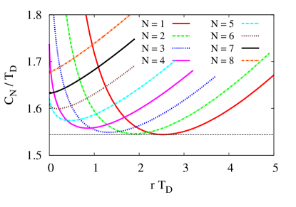
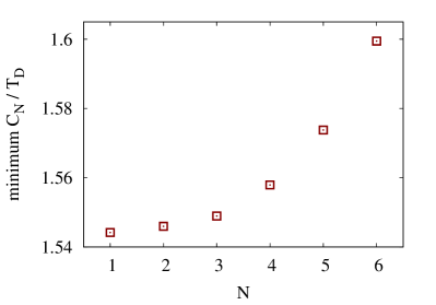
Figure 2: (a) Average search cost $C_{N}$ scaled by the diffusion time $T_{D}$ versus the scaled reset rate $rT_{D}$ in one dimension for various $N$. Each curve represents an average over $10^{9}$ trajectories. The dashed line indicates the minimum cost of 1.544 for $N=1$. (b) The minimum search cost for each $N\leq 6$.

Figure 2 shows the search cost in one dimension as a function of $r$ for $1\leq N\leq 8$. Noteworthy features of the search cost include:

1. The lowest scaled search cost of $1.544$ is achieved by a single searcher that is reset at the scaled optimal rate $r^{*}_{1}\approx 2.540$. At this optimum, there are typically $r^{*}_{1}\langle t_{1}\rangle\approx 3.657$ resets before the searcher reaches the target.

2. For $N=2,3,\ldots 7$, there is a unique, non-zero optimal reset rate $r^{*}_{N}$ for each $N$ that minimizes the search cost and the search time. This optimal rate is generally of the order of the inverse diffusion time between the home base and the target, $T_{D}=x_{0}^{2}/D$. The optimal cost for all $N\leq 5$ is within 2% of the optimal cost for a single searcher.

3. For $N\!\geq\!8$, the search time strictly increases with $r$; that is, no resetting is optimal. This behavior arises because at least one searcher is systematically moving toward the target, once the number of searchers is sufficiently large, so that any resetting increases the search time. The demonstration of the sign change in the initial slope of $\langle t_{N}\rangle$ versus $r$ between $N=7$ and $8$ (see Fig. 3) is given in B.

   

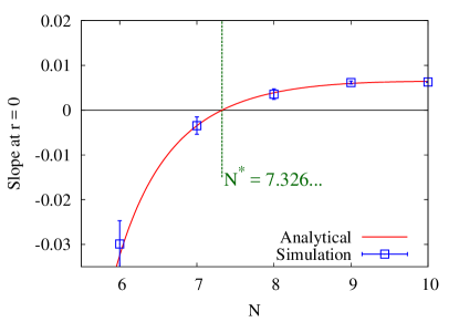
   Figure 3: Slope of the average search time $\langle t_{N}\rangle$ at $r=0$ as a function of $N$ in one dimension when each searcher is independently reset at rate $r$.

4. For $N=1$, the average search time diverges as $r\to 0$. This property reflects the divergence of the first-passage time for a diffusing particle to hit an arbitrary point in one dimension [37, 39]. Since the survival probability for the diffusing particle to not hit the target by time $t$, $S(x_{0},t)$ in Eq. (2a), asymptotically decays as $t^{-1/2}$, we estimate the hitting time for small $r$ as $\int^{1/r}S(x_{0},t)\,dt\sim r^{-1/2}$. This reproduces the behavior that arises from a small-$r$ expansion of search time in Eq. (1).

5. For $N=2$, the search time again diverges as $r\to 0$. Because of the independence of the searchers, the survival probability of the target asymptotically decays as $\big{[}t^{-1/2}\big{]}^{2}=t^{-1}$. In the $r\to 0$ limit, the same argument as that given for $N=1$ leads to an average search time that diverges as $-\ln r$ for $r\to 0$.

6. The probability that the target is not hit by any of $N$ searchers asymptotically decays as $\big{[}t^{-1/2}\big{]}^{N}$. Thus when there are at least 3 searchers, the search time is finite for $r\to 0$,

3 Poisson Resetting in Higher Dimensions

3.1 Three dimensions

There are two important physical differences between the one-dimensional and three-dimensional system: (a) First, the target must have a non-zero size to be detected; we take the target to be an absorbing sphere of radius $a$. (b) Second, the existence of a non-zero target radius introduces an additional parameter—the ratio of the target radius to the radius of the reset point $a/r_{0}$.

In spite of these two complications, the above approach for one dimension can be straightforwardly adapted to three dimensions because of the well-known correspondence between the diffusion equation in three dimensions and in one dimension [40, 39]. Namely, the three-dimensional radial Laplacian operator is related to the one-dimensional Laplacian by $r\,\nabla^{2}_{3d}\,P=\nabla^{2}_{1d}\,(rP)$. Using this mapping, we can write basic quantities for search with resetting in three dimensions in terms of corresponding one-dimensional expressions.

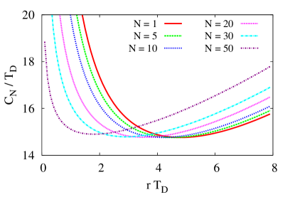
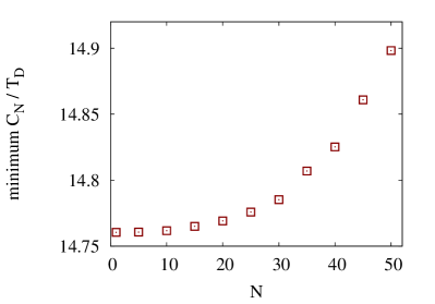
Figure 4: (a) Average scaled search cost $C_{N}/T_{D}$ versus scaled reset rate $rT_{D}$ in three dimensions for various $N$ and for $a/r_{0}=10^{-1}$. The curves for $N=1$ and 5 are averaged over $10^{8}$ trajectories, while those for $N=10,20,30$ and $50$ are averaged over $10^{7}$ trajectories. (b) Minimum search cost as a function of $N$.

Because of computational limitations, most of our numerical results for stochastic resetting in $d=3$ are for the case of $a/r_{0}=10^{-1}$ (Fig. 4). Simulations for different $a/r_{0}$ give a qualitatively similar dependence of the search time and search cost on the reset rate. As in the corresponding one-dimensional system, several features of these results are worth highlighting:

1. For $N\lesssim 10$, the minimum cost changes so slowly with $N$ that is is not possible to determine the value of $N$ at which the minimum cost is achieved. For example, for $N=1$, the minimum cost is $14.760\pm 0.0015$ while for $N=10$, the minimum cost is $14.762\pm 0.0015$. By $N\approx 15$, however, the minimum cost has a systematic increasing trend that is larger than the error bars in the data.

2. In distinction to one dimension, the typical number of reset events before the target is found by a single searcher is of the order of $r_{0}/a$, which can be large. To understand this behavior, we start with the hitting probability $H_{\rm 3d}(r_{0},t)$ that a single searcher that is a distance $r_{0}$ from the center of the target finds it within time $t$ [39]:

   $$H_{\rm 3d}(r_{0},t)=1-S_{\rm 3d}(r_{0},t)=\frac{a}{r_{0}}\operatorname{erfc}{\Big{(}\frac{r_{0}-a}{\sqrt{4Dt}}\Big{)}}\,.$$

   Here $S_{\rm 3d}(r_{0},t)$ is the probability that the searcher does not find the target within time $t$ (see Sec. 4.2). For $r_{0}\gg a$ and reset rate near the optimal value of $D/r_{0}^{2}$, the above hitting probability reduces to $H_{\rm 3d}(r_{0},t)\approx\frac{a}{r_{0}}\text{erfc}(\frac{1}{2})$. Thus for $a/r_{0}\ll 1$, the number of reset events until target is found is of the order of the inverse of this hitting probability, namely, of the order of ${r_{0}}/{a}$.

3. Because of the transience of diffusion in three dimensions, the search time and search cost diverge as $r\to 0$ for any number of searchers. Thus infinitesimal resetting always leads to a more efficient search than no resetting.

3.2 Two dimensions

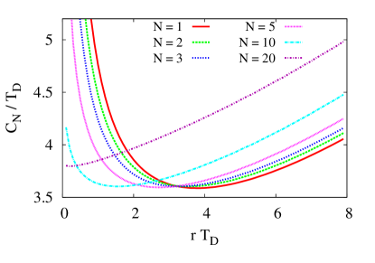
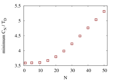
Figure 5: (a) Average scaled search cost $C_{N}/T_{D}$ versus scaled reset rate $rT_{D}$ in two dimensions for various $N$ and for $a/r_{0}=10^{-1}$. The data are averaged over $10^{8}$ trajectories. (b) Minimum search cost as a function of $N$.

In two dimensions, it is practically not feasible to implement an event-driven simulation because the first-passage and hitting probabilities that form the kernel of the event-driven algorithm are not known in closed form as a function of time. (They are known, however, in the Laplace domain [39], and were used in [25, 26] to provide an analytical expression for the search time for the case of a single searcher.)  Thus we implement an alternative simulational approach, as will be discussed in the next section.

The primary features of search with stochastic resetting in two dimensions are (see Fig. 5):

1. Resetting again always leads to a more efficient search compared to the case of no resetting. As in three dimensions, this feature is a consequence of the divergent average search time at $r=0$ in two dimensions for any number of searchers.

2. The dependence of the search cost as a function of reset rate is qualitatively similar to that in three dimensions. The minimum cost is nearly constant for $N\lesssim 10$, with the difference in the cost values for adjacent $N$ values less than the simulation error bars. For example, the minimum costs for $N=1$ and $10$ are $3.59\pm 0.01$ and $3.60\pm 0.01$ respectively, while for $N=15$, the minimum cost in $3.67\pm 0.02$.

4 Event-Driven Simulations

The one- and three-dimensional numerical results are based on an event-driven algorithm that allows us to efficiently simulate $N$ independently resetting searchers. In our approach, each searcher is propagated by a single (typically macroscopic) time step between reset events until one of the searchers finds the target. Thus each update is “useful” in that either the target is found or a reset event occurs. No time is expended in diffusively propagating searchers between resets.

4.1 One dimension

In one spatial dimension, the elemental steps of our algorithm are the following:

1. Start with all the searchers at a distance $x_{0}$ from the target.

2. For each searcher, with the $i^{\rm th}$ one located at $x_{i}$, draw a random time value from the first-passage distribution $F(x_{i},t)$ given in Eq. (2b). Also choose a reset time $t_{r}$ from a Poisson distribution according to the reset rate $Nr$. This gives the time for one of the $N$ searchers to be reset.

3. If the minimum among these $N+1$ times is the reset time, choose a random searcher and reset it to $x_{0}$. Each of the remaining searchers is moved from its current position $x_{i}$ to a new position that is drawn from the conditional probability

   $$P(x_{i},t_{r})=\frac{1}{\sqrt{4\pi Dt_{r}}}\left[e^{-(x_{i}-x_{0})^{2}/4Dt_{r}}-e^{-(x_{i}+x_{0})^{2}/4Dt_{r}}\right]\Big{/}S(x_{0},t_{r})\,,$$

   where $S(x_{0},t_{r})$ is again the probability that a diffusing particle that starts at $x_{0}$ does not hit the target up to time $t_{r}$. The distribution $P(x_{i},t_{r})$ corresponds to the diffusive propagation of each searcher over the time increment $t_{r}$, subject to the constraint that no searcher can reach the target. After all the searchers are moved, increment the elapsed time by the reset time $t_{r}$ and return to step (i).

4. If the minimum among the $N+1$ random times is one of the first-passage times, then the target is found. The total search time is the current elapsed time plus this first-passage time.

4.2 Three dimensions

By exploiting the dimensional reduction of the diffusion equation in three dimensions to one dimension, the algorithm outlined above can be directly adapted to the three-dimensional system. The algorithmic steps of our event-driven simulation are now:

1. Start with all the searchers at a distance $r_{0}$ from the target.

2. For each searcher, with the $i^{\rm th}$ searcher at a radial distance $r_{i}$, draw a random time value from the three-dimensional first-passage distribution to a sphere of radius $a$ [39]:

   $$F_{\rm 3d}(r_{i},t)=\frac{a}{r_{i}}\frac{r_{i}-a}{\sqrt{4\pi Dt^{3}}}\,\,e^{-(r_{i}-a)^{2}/4Dt}\,.$$ (8a)

   Also choose a reset time $$t_{r} Nr$$ from a Poisson distribution with reset rate .

3. If the minimum among these $N+1$ times is the reset time, choose a random searcher and reset it to $r_{0}$. Each of the remaining searchers is moved from its current position $r_{i}$ to a new position that is drawn from the conditional probability

   $$P_{\rm 3d}(r_{i},t_{r})=\frac{r_{i}}{r_{0}}\frac{1}{\sqrt{4\pi Dt_{r}}}\left[e^{-(r_{i}-r_{0})^{2}/4Dt_{r}}-e^{-(r_{i}+r_{0}-2a)^{2}/4Dt_{r}}\right]\Big{/}S(r_{0},t_{r})\,,$$ (8b)

   with survival probability now equal to [39]

   $$S_{\rm 3d}(r_{0},t_{r})=1-\frac{a}{r_{0}}\operatorname{erfc}{\bigg{(}\frac{r_{0}-a}{\sqrt{4Dt_{r}}}\bigg{)}}\,.$$ (8c)

   Here $P_{\rm 3d}(r_{i},t_{r})$ corresponds to diffusive propagation of each searcher over a time $t_{r}$, subject to the constraint that each searcher cannot reach a spherical target of radius $a$. After all the searchers are moved, increment the elapsed time by $t_{r}$ and return to step (i).

4. If the minimum among the $N+1$ random times is one of the first-passage times, then the target is found. The total search time is the current elapsed time plus this first-passage time.

4.3 Two dimensions

As mentioned in the previously, it is impractical to implement an event-driven simulation in two dimensions because the exact expression for the first-passage probability to a circular target of radius $a$ as a function of time is not known in closed form. While this first-passage probability can be expressed as an inverse Laplace transform, the slow convergence properties of this integral render it not useful as the kernel for an event-driven simulation. However, we do know the first-passage probability in the form of a well-converged series to the circumference of a circle centered around the current position of the target. Thus our simulation is based on propagating the searcher to the circumference of a circle whose radius adaptively varies depending on the distance to the target (Fig. 6). This circle should just touch the target, so that the radius of this circle is large when the searcher is far from the target and small when the searcher is close to the target.

For a single searcher that is a distance $b$ from the circumference of the target, the steps in our algorithm are the following (Fig. 6):

1. Draw two random times. One is from the distribution of first-passage times $\mathcal{F}(b,t)$

   $$\mathcal{F}(b,t)=\sum_{n=1}^{\infty}\frac{2}{\mu_{n}{J}_{1}\left(\mu_{n}\right)}e^{-\mu_{n}^{2}Dt/b^{2}}$$ (9)

   to the circumference of a circle of radius $b$ (C). Here $J_{1}$ is the ordinary Bessel function of index 1 and $\mu_{n}$ is the $n^{\rm th}$ zero of this Bessel function. Because the jump distance is large if the searcher is far from the target, little time is spent in simulating the motion of the searcher when it is wandering aimlessly far from the target. The second random time is drawn from the reset time distribution.

2. If the minimum of these two times is the reset time, reset the searcher to $r_{0}$.

3. Otherwise, move the searcher to a random point on the circumference of the circle of radius $b$. If the searcher is within a radius $a(1+\epsilon)$ of the center of the target, then we define the target as being found. If the target is not found after the searcher has been moved, return to step (i).

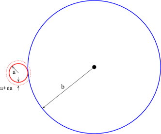
Figure 6: Illustration of a simulation event in two dimensions for a searcher that is a distance $b$ from the circumference of a target of radius $a$.

We need to introduce an absorbing shell of thickness $\epsilon a$ around the target to ensure that the searcher actually finds the target. Clearly, the apparent search time decreases as $\epsilon$ is increased. To determine the appropriate choice of $\epsilon$, we simulate the search with successively smaller values of $\epsilon$ until the results do not change within the statistical errors of the simulation and then use the largest of this set of $\epsilon$ values for simulational efficiency. For the case of $a/r_{0}=10^{-1}$, this value is $\epsilon=10^{-3}$.

By averaging over many trajectories, we construct an accurate numerical estimate for survival probability due to a single searcher, $S_{1}(t)$. Due to the independence of the searchers, we construct the survival probability for $N$ searchers by $S_{N}(t)=\big{[}S_{1}(t)\big{]}^{N}$. The average search time is then given by $\left\langle t_{N}\right\rangle=\int_{0}^{\infty}S_{N}(t)dt$.

5 Deterministic Resetting

We now investigate the situation where all searchers are reset to their starting point after a fixed time $T$. As we shall see, this deterministic resetting typically leads to a more efficient search compared to stochastic reset. Moreover, because all searchers are reset simultaneously, we are able to obtain numerically exact results for the search time for deterministic resetting in both one and three dimensions.

5.1 One dimension

5.1.1 Single searcher.

We follow the renewal approach of Sec. 2 to calculate the average search time for a single searcher that is reset to $x_{0}$ after a fixed time $T$. In this case $R(t)$, the probability that reset time is greater than $t$, is just the Heaviside step function $H(T-t)$, where $H(z)=1$ for $z>0$ and $H(z)=0$ for $z<0$. From Eqs. (3) and (6), we have

$$\begin{split}Q=-\int_{0}^{\infty}dt\,S(x_{0},t)\,\frac{dR(t)}{dt}=S(x_{0},T)\,,\\ T_{d}+T_{r}=\int_{0}^{\infty}dt\,R(t)\,S(x_{0},t)=\int_{0}^{T}S(x_{0},t)\,dt\,.\end{split}$$ (10)

Substituting these expressions into Eq. (5b), the average search time for deterministic resetting of a single searcher is (Fig. 7)

$$\langle t_{1}\rangle =\int_{0}^{T}S(x_{0},t)\,dt/\big{(}1-S(x_{0},T)\big{)}$$

$$=\left[\!\sqrt{\frac{x_{0}^{2}\,T}{\pi D}}\,e^{-{x_{0}^{2}}/{4DT}}-\frac{x_{0}^{2}}{2D}\,\text{erfc}\Big{(}\frac{x_{0}}{\sqrt{4DT}}\Big{)}+T\,\mathrm{erf}\Big{(}\frac{x_{0}}{\sqrt{4DT}}\Big{)}\!\right]\!\bigg{/}\!\mathrm{erfc}\Big{(}\frac{x_{0}}{\sqrt{4DT}}\Big{)}\,.$$ (11)

5.1.2 Multiple searchers.

For multiple searchers, we merely need to use $[S(x_{0},t)\big{]}^{N}$ rather than $S(x_{0},t)$ in Eq. (10) to account for $N$ independent searchers that all must have their hitting time exceed a given threshold. Thus we have

$$\begin{split}Q=-\int_{0}^{\infty}dt\,\big{[}S(x_{0},t)]^{N}\,\frac{dR(t)}{dt}=\big{[}S(x_{0},T)\big{]}^{N}\,,\\ T_{d}+T_{r}=\int_{0}^{\infty}dt\,R(t)\,\big{[}S(x_{0},t)\big{]}N=\int_{0}^{T}\big{[}S(x_{0},t)\big{]}^{N}\,dt\,.\end{split}$$ (12)

Substituting these in (5b), the average search time for $N$ searchers with deterministic reset in one dimension has the simple form

$$\left\langle t_{N}\right\rangle=\frac{\int_{0}^{T}\big{[}S(x_{0},t)\big{]}^{N}dt}{1-\big{[}S(x_{0},T)\big{]}^{N}}\,.$$ (13)

While we can compute the integral in (13) analytically for the cases $N=1,2$ and $N\to\infty$ (D), Mathematica can perform the integration numerically to arbitrary precision to give $\langle t_{N}\rangle$ for any $N$.

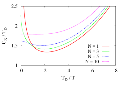
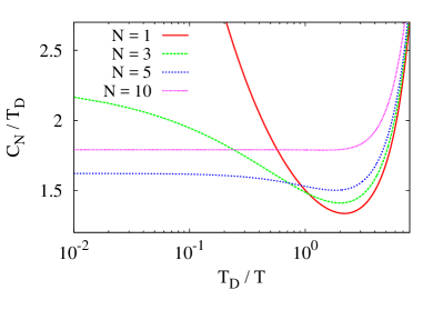
Figure 7: Average search cost scaled by the diffusion time $T_{D}$ versus $T_{D}/T$ in one dimension for various $N$ and for deterministic resetting. The abscissa scale is linear in (a) and logarithmic in (b).

Figure 7 shows the search cost as a function of $1/T$ for representative $N$ values. We plot the search cost versus $1/T$ because $1/T$ plays the same role as the rate $r$ in stochastic resetting. Several new features of the search cost for deterministic reset in one dimension are worth emphasizing:

1. The lowest search cost is achieved by a single searcher (as in stochastic reset) in which the optimal scaled reset time is $T_{1}^{*}/T_{D}\approx 0.458$, leading to an optimal scaled search time $\langle t_{1}\rangle\approx 1.336\,T_{D}$, compared to the optimal cost $1.544\,T_{D}$ from stochastic resetting. This optimal time corresponds to approximately 3 reset events before the target is found.

2. For large $N$, the search cost becomes nearly independent of $1/T$ over a wide range (Fig. 7(b)). This behavior is characterized by progressively more derivatives of the cost with respect to $1/T$ becoming zero as $1/T\to 0$. In particular, the first derivative is zero for $N>4$, the second is zero for $N>6$ and the third is zero for $N>8$. In general, we find that the $k^{\rm th}$ derivative becomes zero for $N=2k+3$. We can understand this pattern of behavior by differentiating Eq. (13) with respect to $1/T$, using Mathematica, to find the leading behavior

   $$\frac{\partial\left\langle t_{N}\right\rangle}{\partial(1/T)} \simeq A_{1}T^{3/2}\Big{(}\operatorname{erf}{\sqrt{{x_{0}^{2}}/{4DT}}}\Big{)}^{N-1}-A_{2}T^{2}\Big{(}\operatorname{erf}{\sqrt{{x_{0}^{2}}/{4DT}}}\Big{)}^{N}$$ (14)

   where $A_{1}$ and $A_{2}$ are $\mathcal{O}(1)$ in $T$. As $1/T\rightarrow 0$, the error function is proportional to its argument, so that the above leading terms scale as a negative power of $T$ for $N>4$ and as a positive power for $N<4$. Analogous behavior arises for higher derivatives.

   

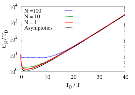
   Figure 8: Comparison between the exact formula (13) and the asymptotic formula (15) for the mean hitting time in one dimension with deterministic reset.

3. For $T_{D}/T\to\infty$, the search time asymptotically increases as $e^{T_{D}/T}$, whereas for stochastic resetting the corresponding $r\to\infty$ behavior is the search time growing as $e^{\sqrt{r}}$. The $e^{T_{D}/T}$ growth has a simple origin. As $T_{D}/T\to\infty$, the probability that one searcher does not reach the target within the reset time $T$ is $S=\text{erf}(x_{0}/\sqrt{4DT})$. The probability that none of the searchers reaches the target within time $T$ is $S^{N}$, so that the probability that at least one of the searchers reaches with time $T$ is $1-S^{N}$. In the limit $T_{D}/T\to\infty$, the asymptotic behavior of this probability is

   $$1-S^{N}\simeq\frac{\sqrt{4DT}\,N\,e^{-x^{2}/4DT}}{\sqrt{\pi}\,x_{0}}\ll 1\,.$$

   The number of reset events until a searcher finds the target is the inverse of this expression. Multiplying by $NT$ gives the asymptotic behavior of the average search cost

   $$\langle C_{N}\rangle\simeq\frac{NT}{1-S^{N}}\simeq\,T\,\sqrt{\frac{\pi x_{0}^{2}}{4DT}}\,\,e^{x_{0}^{2}/4DT}\,.$$ (15)

   This asymptotics matches the numerically exact expression for the search time when $T_{D}/T\gg 1$ (Fig. 8)

5.2 Three dimensions

In three dimensions, we again obtain numerically exact results for deterministic reset for all parameter values and thus can probe the role of the reset time, as well as the parameter $a/r_{0}$ on the search cost and search time. While the qualitative dependence of the search cost and time on $1/T$ is the same for all $a/r_{0}$, there are quantitative anomalies that are worth highlighting.

We again use the correspondence between one-dimensional and three-dimensional diffusion to determine the search time in three dimensions. In the renewal formula (13) for the search time, we now need the first-passage and survival probabilities in three dimensions, $F_{\mathrm{3d}}(r_{0},t)$ and $S_{\mathrm{3d}}(r_{0},t)$, respectively (Eqs. (8a) and (8c)). Substituting these expressions into Eq. (13) and using Mathematica to perform the integrals numerically, we again obtain the search time and cost as a function of $1/T$ for any $N$ with arbitrary precision (Fig. 9).

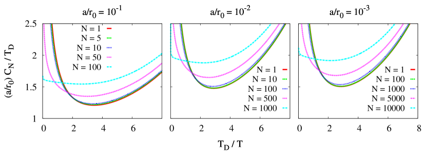
Figure 9: Average search cost scaled by $aT_{D}/r_{0}$ versus $T_{D}/T$ in three dimensions for various $N$ and $a/r_{0}$.

As expected, the search cost is initially a decreasing function of $T_{D}/T$ for any $N$. When $T_{D}/T=0$, a diffusing searcher is transient in three dimensions and does not necessarily find the target; thus the search cost diverges in this limiting case, even when $N$ is large. On the other hand, for $T_{D}/T\to\infty$, the search again becomes inefficient because each searcher is typically reset before it can progress towards the target.

Figure 9 also illustrates a data collapse within each panel when $N\ll r_{0}/a$ and between panels in the limit of $r_{0}/a\gg 1$. This implies that the search cost is independent of $N$ and $a/r_{0}$, for small enough target size and number of searchers, when this cost is scaled by $a/(r_{0}T_{D})$. To derive this behavior, we substitute Eqs. (8a) and (8c) into (13), and approximate the argument of the error function, $(r_{0}-a)/\sqrt{4DT}$, as $\sqrt{T_{D}/4T}$. These steps lead to

$$\left\langle t_{N}\right\rangle=\frac{\int_{0}^{T}\left[1-(a/r_{0})\operatorname{erfc}{\Big{(}\sqrt{T_{D}/4T}\Big{)}}\right]^{N}dt}{1-\left[1-(a/r_{0})\operatorname{erfc}{\Big{(}\sqrt{T_{D}/4T}\Big{)}}\right]^{N}}~{}.$$

In the limit $r_{0}/(aN)\gg 1$, the search cost $\langle C_{N}\rangle=N\langle t_{N}\rangle$ is

$$\left\langle C_{N}\right\rangle=\frac{r_{0}T}{a}\left[\operatorname{erfc}{\left(\sqrt{{T_{D}}/{4T}}\right)}\right]^{-1}\,.$$ (16)

This scaling form implies that plots of $\langle C_{N}\rangle$ versus $1/T$ collapse onto a single curve when $a\left\langle C_{N}\right\rangle/r_{0}$ is plotted against $T_{D}/T$. The asymptotic form (16) may also be derived by merely counting the number of resets until the target is found. The probability of hitting the target within a single reset event by a single searcher is given by,

$$p\equiv 1-S(r_{0},T)=\frac{a}{r_{0}}\operatorname{erfc}{\left(\frac{r_{0}-a}{\sqrt{4DT}}\right)}\,.$$

The probability that any of the $N$ searchers finds the target is $1\!-\!(1\!-\!p)^{N}\simeq Np\equiv P$. Since each of these hitting events is independent, the average number of reset events before one of the searchers reaches the target is $\sum_{n\geq 1}nP(1-P)^{n}=1/P\simeq r_{0}/\big{[}Na\operatorname{erfc}(\sqrt{{T_{D}}/{4T}})\big{]}$. In the limit of large number of resets, the search time is just $T$ times number of resets, as the time for the last segment of the trajectory that actually reaches the target is negligible. This reasoning again leads to Eq. (16).

5.3 Two dimensions

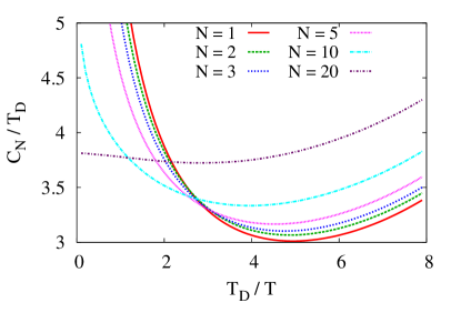
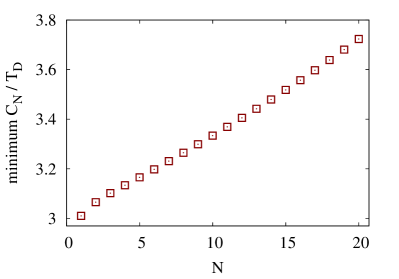
Figure 10: (a) Average scaled search cost $C_{N}/T_{D}$ versus scaled inverse reset time $T_{D}/T$ in two dimensions for various $N$ and for $a/r_{0}=10^{-1}$. Data are averaged over $10^{8}$ trajectories. (b) Minimum search cost as a function of $N$.

In two dimensions however, we are not able to implement the renewal process calculation, as we do not have exact expressions for $S(r_{0},t)$ or $F(r_{0},t)$. Hence, we use the same simulation as in the stochastic reset in $d=2$. As in one and three dimensions, minimum cost is achieved for $N=1$ searcher and the cost monotonically increases with $N$ (Fig. 10).

6 Discussion

In this work, we explored the consequences of superimposed resetting on the performance of stochastic search processes. In this resetting, either one or many searchers are returned to a fixed home base either at a fixed rate or at a fixed reset time. We found a variety of intriguing and sometimes unexpected features. When each searcher is independently reset to the home base at a fixed rate $r$, the search cost is minimal for a single searcher when the reset rate is of the order of the inverse diffusion time $T_{D}=x_{0}^{2}/D$. We also found that resetting always hinders the search for $N\geq 8$ searchers, while for $N\leq 7$, there is an optimal nonzero reset rate for each $N$.

By exploiting the well-known relation between the diffusion equation in one and in three dimensions, we obtained analogous results for search with stochastic resetting in three dimensions. The primary new result for $d=3$ is that the cost of the search is nearly independent of the number of searchers for $N<10$ for the case of $a/r_{0}=10^{-1}$. In two dimensions, we developed an alternative procedure in which we simulate the target survival probability in the presence of a single searcher and then take the $N^{\rm th}$ power of this quantity to obtain the target survival probability in the presence of $N$ searchers. In this case, similar to three dimensions, the cost is nearly independent of the number of searchers up to $N=10$ and for $N>10$, the cost increases monotonically.

We also explored a related model in which all searchers are simultaneously reset to the home base after a fixed operation time $T$. This deterministic resetting is theoretically and computationally simpler than stochastic resetting, and we are able to obtain explicit formulae for the average search time for any $N$ that can be numerically integrated to arbitrary precision. In one dimension, deterministic resetting gives a search time that becomes independent of the reset time $T$ when $N$ is sufficiently large, a behavior that can be understood from the small-$r$ behavior of the search time. In three dimensions, we showed by a simple extremal argument that the search cost versus $1/T$ becomes independent of $N$.

There are a wide range of extensions of the basic model to practically and theoretically interesting situations. It would be worthwhile to extend search with resetting to the cases where either the target is diffusing and/or the target is mortal [42, 43, 44, 45]. These generalizations would naturally describe, e.g., the occupants of a lifeboat that is adrift in the ocean. When the target is also moving, the basic question is again whether the reset helps or hinders the search. For a mortal target with any reasonable distribution of mortality, there will always be a non-zero probability that the target will die before being found and the relevant issue is to construct appropriate criteria that lead to a well-defined optimization problem.

Financial support for this research was also provided in part by the grants DMR-1623243 from the National Science Foundation (UB and SR), from the John Templeton Foundation (CDB and SR), and Grant No. 2012145 from the United States—Israel Binational Science Foundation (UB). We also thank B. Meerson for helpful discussions and S. Reuveni for useful comments on the manuscript.

Added Note: As final revisions were being made, we became aware of related work [46], in which the authors mathematically showed that deterministic reset leads to the smallest search time for the case of a single searcher, as we also observed.

Appendix A The Probability Distribution

The full description for a static target and one searcher that is stochastically reset to $x_{0}$ can be obtained from the time-dependent probability distribution $\rho(x,t)$. Its evolution is governed by the diffusion equation, supplemented by terms that account for the resetting:

$$\rho_{t}=D\rho_{xx}-r\rho+r\delta(x-x_{0})\int_{0}^{\infty}\rho(x,t)\,dx\,.$$ (17)

Here $r\rho$ accounts for the loss of probability at rate $r$ at position $x$ due to the resetting, while the integral accounts for the gain of probability at the reset point $x_{0}$. The amplitude of this gain term equals the total probability that the target has not yet been found, which is less than 1 and also decreasing with time. We solve this equation, subject to the absorbing boundary condition $\rho(0,t>0)=0$, corresponding to the loss of probability whenever the target at the origin is reached. For simplicity, we consider the initial condition $\rho(x,t\!=\!0)=\delta(x\!-\!x_{0})$.

To solve Eq. (17), we first Laplace transform it to give

$$s\rho-\delta(x-x_{0})=D\rho^{\prime\prime}-r\rho+r\delta(x-x_{0})\int_{0}^{\infty}\rho(x,s)\,dx\,.$$ (18)

Here $\rho=\rho(x,s)$ is the Laplace transform of $\rho(x,t)$ and the prime denotes differentiation with respect to $x$. For $x\neq x_{0}$, we must solve $\rho^{\prime\prime}=\left(\frac{s+r}{D}\right)\rho\equiv\alpha^{2}\rho$, with general solution

$$\rho(x,s)=\begin{cases}A\,e^{\alpha x}+B\,e^{-\alpha x}&\qquad x<x_{0}\,,\\ C\,e^{-\alpha x}&\qquad x>x_{0}\,.\end{cases}$$

For $x>x_{0}$, only the decaying exponential appears so that the probability distribution does not diverge as $x\to\infty$.

The absorbing boundary condition at the origin immediately gives $A+B=0$, which simplifies the density in the range $x<x_{0}$ to $\rho=A\,\textrm{sinh}\,\alpha x$. Continuity of the probability distribution at $x_{0}$ gives the condition $A\,\textrm{sinh}\,\alpha x_{0}=C\,e^{-\alpha x_{0}}$, which we use to eliminate $C$. After some standard and simple steps, the form of $\rho(x,s)$ for $x<x_{0}$ and $x>x_{0}$ can be expressed more symmetrically as

$$\rho(x,s)=\begin{cases}A\,{\displaystyle\frac{\textrm{sinh}\,\alpha x}{\textrm{sinh}\,\alpha x_{0}}}&\qquad x<x_{0}\,,\\[14.45377pt] A\,e^{-\alpha(x-x_{0})}&\qquad x>x_{0}\,,\end{cases}$$ (19)

which is manifestly continuous at $x=x_{0}$.

The constant $A$ is determined by the joining condition, which is obtained by integrating (18) over an infinitesimal region that includes $x_{0}$:

$$-1=D\left(\rho_{+}^{\prime}-\rho_{-}^{\prime}\right)+r\int_{0}^{\infty}\rho(x^{\prime},s)\,dx^{\prime}\,.$$ (20)

Here $\rho_{+}^{\prime}$ is the gradient of $\rho$ as $x\to x_{0}^{+}$ and similarly for $\rho_{-}^{\prime}$. Using Eq. (19), we have

$$\begin{split}\rho_{+}^{\prime}&=-A\,\alpha\,\,e^{-\alpha(x-x_{0})}\Big{|}_{x=x_{0}}=-A\,\alpha\,,\\ \rho_{-}^{\prime}&=A\,\alpha\,\frac{\textrm{cosh}\,\alpha x}{\textrm{sinh}\,\alpha x_{0}}\Big{|}_{x=x_{0}}=A\,\alpha\,\,\textrm{coth}\,\alpha x_{0}\,.\end{split}$$ (21)

We also need

$$\begin{split}\int_{0}^{\infty}\rho(x^{\prime},s)\,dx^{\prime}&=\int_{0}^{x_{0}}A\,\frac{\textrm{sinh}\,\alpha x^{\prime}}{\textrm{sinh}\,\alpha x_{0}}\,dx^{\prime}+\int_{x_{0}}^{\infty}A\,\,e^{-\alpha(x^{\prime}-x_{0})}\,dx^{\prime}\,,\\ &=\frac{A}{\alpha}\left[\frac{(\textrm{cosh}\,\alpha x_{0}-1)}{\textrm{sinh}\,\alpha x_{0}}+1\right]\,.\end{split}$$ (22)

Substituting the above into the joining condition gives, after straightforward algebra,

$$A=\frac{\textrm{sinh}\,\alpha x_{0}}{D\alpha\,e^{\alpha x_{0}}+\frac{r}{\alpha}\big{(}1-e^{\alpha x_{0}}\big{)}}\,.$$ (23)

This, together with Eq. (19), gives the probability distribution in the Laplace domain.

From this solution, the Laplace transform of the flux to the origin is:

$$j(0,s) =D\rho(x,s)^{\prime}\Big{|}_{x=0}=\frac{DA\alpha}{\textrm{sinh}\,\alpha x_{0}}\,,$$

$$=\left[e^{\alpha x_{0}}+\frac{r}{D\alpha^{2}}\big{(}1-e^{\alpha x_{0}}\big{)}\right]^{-1}\,.$$ (24)

By definition, $j(0,s)$ is also the moment generating function

$$j(0,s) =\int_{0}^{\infty}j(0,t)\,e^{-st}\,dt\,,$$

$$=\int_{0}^{\infty}j(0,t)\big{[}1-st+\tfrac{1}{2}(st)^{2}-\ldots\big{]}\,,$$

$$=1-s\langle t\rangle+\tfrac{1}{2}s^{2}\langle t^{2}\rangle-\ldots\,.$$ (25)

Expanding (A) in a power series in $s$, we obtain the results quoted in Eq. (1).

As a byproduct, the survival probability of the searcher in the Laplace domain, $S_{1}(x_{0},s)$ (which coincides with the survival probability of the target) is the spatial integral of $\rho(x,s)$ in Eq. (22). Using (23), and after some simple algebra, we obtain

$$S_{1}(x_{0},s)=\frac{1-e^{-\alpha x_{0}}}{s+re^{-\alpha x_{0}}}\,,$$ (26)

as first obtained in Ref. [24, 25] by different means.

Appendix B Slope of $\langle t_{N}\rangle$ for $r\to 0$

Because of the independence of the searchers, the probability that the target is not found by $N$ searchers within time $t$, $S_{N}(t)$, is just $\big{[}S_{1}(t)\big{]}^{N}$. Thus the slope of the average search time at $r=0$ is

$$\frac{d\langle t_{N}\rangle}{dr}\bigg{|}_{r=0} =\frac{d}{dr}\int_{0}^{\infty}\big{[}S_{1}(t)\big{]}^{N}\,dt\,\,\bigg{|}_{r=0}$$

$$=\int_{0}^{\infty}N\,\,\big{[}S_{1}(t,r\!=\!0)\big{]}^{N-1}\,\,\frac{dS_{1}(t,r)}{dr}\,\,dt\,\bigg{|}_{r=0}$$ (27)

Since we just need the slope at $r=0$, we expand the Laplace transform $S_{1}(x_{0},s)$ in (26) to first order in $r$ to give

$$\lim_{r\to 0}S_{1}(x_{0},s)=\frac{1}{s}\left[1-e^{-x_{0}\sqrt{{s}/{D}}}+\frac{r}{s}\,e^{-x_{0}\sqrt{{s}/{D}}}\left(x_{0}\sqrt{{s}/{4D}}-1+e^{-x_{0}\sqrt{{s}/{4D}}}\right)\right]$$ (28)

Using Mathematica, the Laplace inverse of the above expression is

$$\lim_{r\to 0}S_{1}(x_{0},t)= \frac{rx_{0}^{2}}{D}+2rx_{0}\sqrt{\frac{t}{\pi D}}\left(e^{-{x_{0}^{2}}/{4Dt}}-e^{-{x_{0}^{2}}/{Dt}}\right)$$

$$+\left(1+rt+\frac{rx_{0}^{2}}{D}\right)\mathrm{erf}\left(\frac{x_{0}}{\sqrt{4Dt}}\right)-\left(rt+\frac{2rx_{0}^{2}}{D}\right)\mathrm{erf}\left(\frac{x_{0}}{\sqrt{Dt}}\right)\,.$$ (29)

Differentiating Eq. (B) with respect to $r$ and substituting in (B) gives

$$\frac{d\langle t_{N}\rangle}{dr}\bigg{|}_{r=0}\!\!\!=N\,T_{D}^{2}\int_{0}^{\infty}\!\left[\mathrm{erf}{\Big{(}\frac{1}{\sqrt{4\tau}}\Big{)}}\right]^{N-1} \!\left\{\!1+\sqrt{\frac{4\tau}{\pi}}\left(e^{-{1}/{4\tau}}-e^{-{1}/{\tau}}\right)\right.$$

$$+\left.(\tau\!+\!1)\,\mathrm{erf}{\Big{(}\frac{1}{\sqrt{4\tau}}\Big{)}}-(\tau\!+\!2)\,\mathrm{erf}{\Big{(}\frac{1}{\sqrt{\tau}}\Big{)}}\!\right\}d\tau$$ (30)

where again $T_{D}=x_{0}^{2}/D$. Evaluating the integral numerically shows that the initial slope changes sign at $N\approx 7.326477\ldots$ (see Fig. 3). Thus for $N\leq 7$ searchers, resetting at a non-zero optimal rate speeds up the search compared to no resetting, while for $N\geq 8$, resetting always hinders the search.

Appendix C Survival probability from an absorbing circle

To find the survival probability from an absorbing circle of radius $R$ centered around the origin, with the initial condition $r_{0}=r$, we begin with the diffusion equation in two dimensions,

$$\frac{\partial S(r,t)}{\partial t}=D\nabla^{2}S(r,t)=D\left(\frac{\partial^{2}S(r,t)}{\partial r^{2}}+\frac{1}{r}\frac{\partial S(r,t)}{\partial r}\right)$$ (31)

Due to circular symmetry, the survival probability is independent of the polar angle, and so we have kept only the radial term of the Laplacian operator in 2d. Assuming separation of variables and defining $S(r,t)=\mathcal{R}(r)\mathcal{T}(t)$ and re-arranging the terms, we get

$$\frac{\dot{\mathcal{T}}}{D\mathcal{T}}=\frac{\mathcal{R}^{\prime\prime}}{\mathcal{R}}+\frac{1}{r}\frac{\mathcal{R}^{\prime}}{\mathcal{R}}$$ (32)

where the over-dot refers to derivative w.r.t $t$ and prime refers to derivative w.r.t $r$. Equating both sides to a negative constant $-\mu^{2}$, we obtain

$$\mathcal{T}(t)=e^{-\mu^{2}Dt}\quad\text{and}\quad r^{2}\mathcal{R}^{\prime\prime}+r\mathcal{R}^{\prime}-\mu^{2}r^{2}=0$$ (33)

The equation for $\mathcal{R}(r)$ is in the form of a Bessel equation of order $0$, giving us the general solution,

$$S(r,t)=\sum_{\mu}A_{\mu}J_{0}(\mu r)e^{-\mu^{2}Dt}$$ (34)

Applying the absorbing boundary condition, $S(r=R,t)=0$, we get $\mu=\mu_{n}/R$ where $\left\{\mu_{n}\right\}$ are the zeroes of $J_{0}$

$$S(r,t)=\sum_{n}A_{n}J_{0}\left(\frac{\mu_{n}r}{R}\right)e^{-\mu^{2}Dt}$$ (35)

To calculate the coefficients $A_{n}$, we use the orthogonality condition of the Bessel functions [41] and the initial condition $S(r,t=0)=1\,\forall r<R$. Using Eq. (35) at $t=0$ and multiplying both sides by $(r/R)J_{0}(\mu_{m}r/R)$ and integrating with respect to $r/R$ we get,

$$\int_{0}^{1}\frac{r}{R}J_{0}\left(\mu_{m}\frac{r}{R}\right)d\left(\frac{r}{R}\right)=\sum_{n}\int_{0}^{1}A_{n}\frac{r}{R}J_{0}\left(\mu_{m}\frac{r}{R}\right)J_{0}\left(\frac{\mu_{n}r}{R}\right)d\left(\frac{r}{R}\right)=\frac{A_{n}}{2}\left[J_{1}\left(\mu_{n}\right)\right]^{2}$$ (36)

Integrating the left-hand side with Mathematica and re-arranging terms, we get,

$$A_{n}=\frac{2}{\mu_{n}J_{1}(\mu_{n})}$$ (37)

Finally, we require the survival probability when starting from the center of the absorbing circle, so substituting $r=0$, we get

$$S(r=0,t)=\sum_{n}\frac{2}{\mu_{n}J_{1}(\mu_{n})}e^{-\mu_{n}^{2}Dt/R^{2}}$$ (38)

Appendix D Search Time for Deterministic Reset for $N=2$ and $N=\infty$

We start with the general expression (13) for the average search time in deterministic search:

$$\left\langle t_{N}\right\rangle=\frac{\int_{0}^{T}\big{[}S(t)\big{]}^{N}dt}{1-\big{[}S(T)\big{]}^{N}}\,.$$ (39)

In terms of $u\equiv x_{0}^{2}/4DT=T_{D}/4T$, the integral $\int_{0}^{T}\big{[}S(t)\big{]}^{N}dt$ can be written as

$$\frac{x_{0}^{2}}{2D}\int_{u}^{\infty}\frac{\text{erf}(z)^{N}}{z^{3}}\,dz\equiv\tfrac{1}{2}\,T_{D}\,I\,.$$ (40)

Repeatedly integrating by parts to reduce the power of the factor in the denominator, we obtain

$$I=\Big{(}1\!+\!\frac{1}{2u^{2}}\Big{)}\text{erf}(u)^{N}\!+\!\frac{N}{\sqrt{\pi}\,u}e^{-u^{2}}\text{erf}(u)^{N-1}\!-\!1\!+\!\frac{2}{\pi}N(N\!-\!1)\!\int_{u}^{\infty}\!\!\!\text{erf}(z)^{N-2}\,e^{-2z^{2}}\,\frac{dz}{z}\,.$$ (41)

For the case of $N=2$, the last integral is

$$\int_{u}^{\infty}e^{-2z^{2}}\,\frac{dz}{z}=\Gamma(0,2u^{2})\,,$$

where $\Gamma(a,b)$ is the incomplete Gamma function [41]. Assembling the above results, the average search time for $N=2$ searchers is

$$\langle t_{2}\rangle=\frac{T_{D}}{2}\,\frac{\displaystyle{\left[\Big{(}1+\frac{1}{2u^{2}}\Big{)}\text{erf}(u)^{2}+\frac{2}{\sqrt{\pi}\,u}e^{-u^{2}}\text{erf}(u)-1+\frac{2}{\pi}\Gamma(0,2u^{2})\right]}}{1-\text{erf}(u)^{2}}\,.$$ (42)

In the limit $N\to\infty$, the search time becomes arbitrarily small so that eventually the reset time $T$ is larger than the search time. In this limit, we may set $T=\infty$, or equivalently, $u=0$ in Eq. (40). Thus Eq. (39) reduces to [45]

$$\left\langle t_{N}\right\rangle=\frac{T_{D}}{2}\int_{0}^{\infty}\frac{\text{erf}(z)^{N}}{z^{3}}\,dz\simeq\frac{T_{D}}{4\ln N}\,.$$ (43)

In this limiting case, the average search time no longer depends on the reset time.

References

- [1] For a recent review from the physics perspective, see, e.g., O. Bénichou, C. Loverdo, M. Moreau, and R. Voituriez, Rev. Mod. Phys. 83, 81 (2011).
- [2] O. G. Berg, R. B. Winter and P. H. Von Hippel, Biochem. 20, 6929 (1981).
- [3] P. H. Von Hippel, Ann. Rev. Biophys. Biomol. Struct. 36, 79 (2007).
- [4] L. Mirny, Nature Physics 4, 93 (2008).
- [5] E. L. Charnov, Theor. Popul. Biol. 9, 129 (1976).
- [6] W. J. Bell, Searching Behaviour: the Behavioural Ecology of Finding Resources (Chapman and Hall, London, 1991).
- [7] W. J. O’Brien, H. I. Browman, and B. I. Evans, Am. Sci. 78, 152 (1990).
- [8] G. M. Viswanathan, S. V. Buldyrev, S. Havlin, M. G. E. Da Luz, E. P. Raposo, and H. E. Stanley, Nature 401, 911 (1999).
- [9] O. Bénichou, C. Loverdo, M. Moreau, and R. Voituriez, Phys. Rev. E 74, 020102 (2006).
- [10] H. R. Richardson and L. D. Stone, Naval Research Logistics Quarterly 18, 141 (1971).
- [11] J. R. Frost and L. D. Stone, http.//www.rdc.uscg.gov/reports/2001/cgd1501dpexsum.pdf.
- [12] M. F. Shlesinger, J. Phys. A: Math. Theor. 42, 2009.
- [13] G. Viswanathan, M. G. E de Luz, E. P. Raposo, and H. E. Stanley, The Physics of Foraging (Cambridge University Press, Cambridge, England, 2011).
- [14] C. Mejía-Monasterio, G. Oshanin, and G. Schehr, J. Stat. Mech. P06022 (2011)
- [15] T. G. Mattos, C. Mejía-Monasterio, R. Metzler, and G. Oshanin, Phys. Rev. E 86, 031143 (2012).
- [16] M. F. Shlesinger and J. Klafter, in On growth and forms, edited by H. E. Stanley and N. Ostrowski (Martinus Nijhof Publishers, Amsterdam, 1986), pp. 279–283.
- [17] O. Bénichou, M. Coppey, M. Moreau, P.-H. Suet, and R. Voituriez, Phys. Rev. Lett. 94, 198101 (2005).
- [18] O. Bénichou and S. Redner, Phys. Rev. Lett. 113q, 238101 (2014).
- [19] M. Chupeau, O. Bénichou, and S. Redner, arXiv:1605.00892.
- [20] R. B. Winter and P. H. Von Hippel, Biochem. bf 20 6948 (1981).
- [21] R. B. Winter, O. G. Berg, and P. H. Von Hippel, Biochem. 20, 6961 (1981).
- [22] S. E. Halford and J. F. Marko, Nucleic Acids Res. 32, 3040 (2004).
- [23] T. Hu, A. Y. Grosberg and B. I, Shklovskii, Biophys. J. 90, 2731 (2006).
- [24] M. R. Evans and S. N. Majumdar, Phys. Rev. Lett. 106, 160601, (2011).
- [25] M. R. Evans and S. N. Majumdar, J. Phys. A: Math. Theor. 44, 435001 (2011).
- [26] M. R. Evans and S. N. Majumdar, J. Phys. A: Math. Theor. 47, 285001 (2014).
- [27] M. Montero and J. Villarroel, Phys. Rev. E 87, 012116 (2013).
- [28] O. H. Abdelrahman and E. Gelenbe, Phys. Rev. E 87, 032125 (2013).
- [29] D. Boyer and C. Solis-Salas, Phys. Rev. Lett. 112, 240601 (2014).
- [30] C. Christou and A. Schadschneider, J. Phys. A: Math. Theor. 48, 285003 (2015)
- [31] D. Campos and V. Méndez, Phys. Rev. E 92, 062115 (2015).
- [32] S. N. Majumdar, S. Sabhapandit, and G. Schehr, Phys. Rev. E 92, 052126 (2015).
- [33] A. Pal, Phys. Rev. E 91, 012113 (2015).
- [34] L. Kusmierz and E. Gudowska-Nowak, Phys. Rev. E 92, 052127 (2015).
- [35] T. Rotbart, S. Reuveni, and M. Urbakh, Phys. Rev. E 92, 060101 (2015).
- [36] S. Eule and J. J. Metzger, New J. Phys. 18, 33006 (2016).
- [37] W. Feller, An Introduction to Probability Theory and Its Applications, (Wiley, New York, 1968).
- [38] S. Reuveni, Phys. Rev. Lett. 116, 170601 (2016).
- [39] S. Redner, A Guide to First-Passage Processes (Cambridge University Press, Cambridge, England, 2001).
- [40] S. Chandrasekhar, Rev. Mod. Phys. 15, 1 (1943).
- [41] M. Abramowitz and I. A. Stegun, Handbook of Mathematical Functions, (Dover, New York, 1972).
- [42] S. B. Yuste, E. Abad, and K. Lindenberg, Phys. Rev. Lett. 110, 220603 (2013).
- [43] E. Abad, S. B. Yuste, and K. Lindenberg, Phys. Rev. E 88, 062110 (2013).
- [44] D. Campos, E. Abad, V. Méndez, S. B. Yuste, and K. Lindenberg, Phys. Rev. E 91, 052115 (2015).
- [45] B. Meerson and S. Redner, Phys. Rev. Lett. 114, 198101 (2015).
- [46] A. Pal, A. Kundu, and M. R. Evans, J. Phys. A: Math. Theor. 49, 225001 (2016).