Explicit Time Mimetic Discretiztions

Abstract

This paper is part of a program to combine a staggered time and staggered spatial discretization of continuum mechanics problems so that any property of the continuum that is proved using vector calculus can be proven in an analogous way for the discretized system. It is required that the discretizations be second order accurate and have a conserved quantity that approximates the energy for the system and guarantees stability for a reasonable constraint on the time step. It is also require that the discretization is time explicit so as to avoid the solution of large system of possibly nonlinear algebraic equations. The well known Yee grid discretization of Maxwell’s equations is the same as discretization described here and is an early example of using a staggered space and time grid .

Motivation of the discussion begins by studying the staggered time or leapfrog discretization of the harmonic oscillator and use this to introduce the modification of the energy that is conserved. Next systems of linear equations are used to motivate the definition of the modified energy for more complex systems of ordinary differential equations and then apply these ideas to the scalar wave equation in one spatial dimension. Discretizing the three dimensional scalar wave and Maxwell’s equations shows the power of the mimetic method. Because the spatial discretization is mimetic, the divergence of the electric and magnetic fields are constant when there are no sources. Using the mimetic properties the proof of this trivial and is essentially the same as in the continuum.

Updated versions of this paper will appear at arXiv.

Key Words: mimetic discretization, leapfrog, energy conservation

1 Introduction

The first 7 section have been rewritten. Sections 8, 9, and 10 are to be done soon.

The main goal is to show that mimetic finite difference spatial discretizations can be combined with an explicit finite difference time discretizations to discretize wave equations to produce stable second-order accurate simulations and to create a general method for extending mimetic discretizations to model inhomogeneous and anisotropic materials. The mimetic spatial discretizations require the use of two grids where the corners of cells in one grid are the same points as the centers of the cells in the other grid.

The time discretizations require that the wave equation be written as a first order system and then the leapfrog discretization is used for the system each equation. An early example of this type of time discretization was given by Yee [57]. Most importantly, it is shown how to derive a discrete quantity that is conserved by the solution of the disctrized wave equation and also provides a second order accurate in time approximation to the energy of the waves and is positive for a sufficiently small time step.

Mimetic spatial discretizations have been used extensively to create simulation programs for problems in continuum mechanics, see [31] and the volume [27] in which this work appeared. They have also been used to model inhomogeneous and anisotropic materials in two dimensions [22, 21]. More recently mimetic methods have been used in Magnetohydrodynamics [28, 29] For a comparison of mimetic finite difference, finite volume and finite element discretizations see [5].

The spatial discretization studied here are extensions of those described in [43] where it is shown that mimetic discretizations of the gradient, curl and divergence satisfy all of the important properties of the continuum operators. For example the discrete divergence of the discrete curl operator is identically zero and the adjoint of the discrete gradient is the minus the discrete divergence. To extend this work to anisotropic materials it is critical that in three dimensions the anisotropic properties of many important materials are describe by a $3\times 3$ symmetric positive definite matrix [35], see Chapter 4 Sections 1 and 4 for the permittivity tensor and Chapter 11 Section 5 for heat flow. Additionally, [31, 7, 20, 25] discuss the incorporation of material properties into mimetic discretizations using symmetric positive definite matrices.

Sections 2, 3 and 4 show how to create time conserved quantities for leapfrog time discretizations for successively more complex problems. Section 2 discusses the harmonic oscillator, section 3 discusses constant coefficient linear systems of ordinary differential equations while Section 4 introduces a staggered in time and space discretization for the one dimensional wave equation. It is important that the conserved quantities depend on the time step but converge second order to a conserved quantity for the continuum problem. Simulations show that the quantity is conserved to at least one part in $10^{14}$.

In Section 2 begins with the harmonic oscillator for which it is well known that the implicit Crank-Nicolson discretization conserves a discrete energy, see Appendix A. The oscillator equations are written as a first order system and discretized using a leapfrog scheme. Then the continuum energy or Hamiltonian for oscillator are approximated to make a conserved quantity. Simulations show that this quantity is conserved to one part in $10^{15}$, see StaggeredOscillator.m. Keeping the conserved quantity positive gives a time step constraint for stability that is far less restrictive than the constraint for accuracy.

In Section 3 the discussion of the harmonic oscillator is extended to finite and infinite systems of linear ordinary differential equations that are wave equations. Such equations have conserved continuum quantities and their leapfrog discretizations are shown to also have an approximate conserved quantities analogous to that of the harmonic oscillator. These systems are set up to be analogous to the discrete systems obtained from the mimetic discretizations of continuum wave equations. The equations studied are are important motivation for extending the harmonic oscillator discretization to partial differential equations. Again simulations show that the approximate quantities are conserved to about 2 parts in $10^{15}$, see SystemsODE.m.

In Section 4, the scalar wave equation in one space dimension is written as a system of two first order equations and discretized using a grid staggered in space and time. A natural continuum conserved quantity which implies that the classical energy is conserved is introduced. The first order system is discretized using a staggered space time discretization like those used in Yee method [57]. The discrete conserved quantities are extended to cover this 1D case. Simulation show that the new quantities are conserved to one part in $10^{14}$, see OneDWave.m. This provides insight into how to combine mimetic time and spatial discretizations.

Next Sections 5, 6, and 7 discuss three dimensional continuum second order differential operators for anisotropic and inhomogeneous materials that are then used to define general scalar and vector wave equations. The main difference between the discussion here and that in [43] is the introduction of variable material properties.

Section 5 reviews some continuum wave equations in 3 dimensions when the material properties are constant. The main issue is understanding the role of the spatial dimension for distance $d$ plays in the partial differential equations. The scalar and vector wave equations, the elastic wave equation and Maxwell’s equations are introduced and a conserved quantity is given for each equation.

In Section 6 continuum second order differential operators for anisotropic and inhomogeneous materials are introduced. The main idea is to use the notion of a double exact sequence and diagram chasing to define a large class of second order spatial differential operators that can be used to define wave equations. This idea is motivated by the exact sequences used in differential geometry. A knowledge of differential forms is not required for understanding this material but can be helpful [1]. A discrete double exact sequence is critical for the discussion of discretizations using staggered grids. Importantly, the analogous discrete double exact sequence cannot be reduced to a single sequence. The paper [38], Figure 9, uses a double exact sequence that is called a De Rham complex.

Additionally, weighted inner products for scalar and vector functions are introduced and used to define adjoint operators and to show that the second order operators are either positive or negative. The main difference between the discussion here and that in [43] is the introduction of variable material properties. This discussion depends heavily on the spatial units of the dependent variables, the differential operators, and the material properties.

In Section 7 the second order differential operators defined in the previous section are combined with a second time derivative to define several types of wave equations with variable material properties. The second order equations are written as a first order system that has properties similar to the systems studied earlier. This then gives an automatic definition of a conserved quantity. The conserved quantity can be used to easily show that energy is conserved. At the end of the section Maxwell’s equations and the general elastic wave equations examples are studied.

The material below to be revised soon!

In Section 8 primal and dual staggered grids in 3D are introduced. These grids are the same as those introduce by Yee [57] in 1966 to discretize Maxwell’s equations. Consequently there are two types of scalar fields and two types of discrete vector fields. The differential operators divergence, gradient and curl are discretized as in [43]. Because two grids are used there are two of each of the first order discrete operators ${\vec{\nabla}\boldsymbol{\cdot}}$, ${\vec{\nabla}\times}$ and ${\vec{\nabla}}$. Additionally it is shown how to discretize the material properties. This section continues by defining discrete inner products and adjoint operators critical for understanding important properties of the discrete operators. Note that the paper [32] also used a dual grid differential form method to discretize the Navier-Stokes Equations. For an introduction to the relationship of vector calculus to differential forms see the notes [1].

In Section 9 the scalar wave equation and Maxwell’s equations are discretized for constant scalar material properties and constant time the identity for matrix material properties. This is actually a easy task. There are programs [43] available for computing the action of the divergence, curl on discrete vector fields and the gradient on discrete scalar fields. As there are two types of fields so there are two types of each discrete operator. Additionally a with a bit of algebra a conserved quantity similar to the ones in the previous sections can be computed. Simulation show that the conserved quantity is constant to one part in $10^{15}$, see ScalarWave.m. Also the curl of the velocity field is constant to one part in $10^{13}$. So everything works in the case of the scalar wave equation and Maxwell’s equations with constant material properties.

In Section 9.2 we show how to create a conserved quantity for Maxwell’s equations that is constant to one in $10^{15}$, and also show that the divergence of the electric and magnetic fields are constant to one part in $10^{13}$, see Maxwell.m.

Should section 10 be an appendix?

1.1 Notes

For the latest, see the minisimposium at a recent SIAM meeting [48]. For more information on steady state problems see [30] For an idea of the difficulties encountered in discretizing Maxwell’s equations see [10]. Others have used approximate quantities to study time discretizations [19, 18, 13, 16, 42]. It appears that most of the energy preserving methods are implicit, but by introducing additional variables, explicit methods that conserve a modified energy are discussed in [50].

One complexity of mimetic spatial discretizations is caused by having primal and dual grids. This is leads to there being a primal gradient, curl, and divergence and dual gradient, curl and divergence. The dual operators are labeled with a star $\star$. This complexity was already present in the paper by Yee [57] which has evolved into the FDTD discretization method [56].

There are several minor problems caused by writing wave equations as a second order differential equations or as a system of two first order equations. For example second order equations are not exactly equivalent to first order system. Additionally, for the discrete equations there are problems in converting the initial data for the second order equations to data for the first order equations and vice versa. Additionally, because the equations studied are linear, if they conserve some quantity, they will conserve infinitely many quantities and thus there are choices in what conserved quantity to study. For the first order system there is a natural primitive conserved quantity.

This paper was inspired by the papers [54] and [57]. We note that in [47] (see equation (45)) the same stability constraint was found as the one in this paper for conserving the classical energy by modifying the discretization of Maxwell’s equations. In [17] an implicit (ADI) method is developed that has a modified energy that is similar to the one used here but the added term is positive while the added term here is negative. For a finite element approach that produce many of the same results that as in this paper see [51, 6].

The paper [46] gives an overview of energy conserving methods for Navier-Stokes equations and develops some implicit Runge-Kutta methods for doing this. The thesis [8] addresses energy conservation for turbulent flows. For a differential forms approach to discretization see [40, 52] and additionally for multisympletic time integration approach to Maxwell’s equations see [49]. For two dimensional problems see [9, 39, 37, 44, 12, 33, 23, 24]. The papers [53, 54] take a novel approach to finding discrete models. For a finite-element approach to vector wave equations see Section 2.3.2 of [3].

For isotropic and homogeneous materials, simulations show that the three dimensional scalar wave equation and Maxwell’s equations without sources the approximate energy is constant to less than one part in $10^{15}$. Additionally, for the scalar wave equation the curl of the velocity is constant to less than one part in $10^{13}$ and the divergence of the electric and magnetic fields are constant to less than one part in $10^{13}$, see ScalarWave.m and Maxwell.m.

For higher order mimetic methods, see [45].

2 The Harmonic Oscillator

The goal is to use the discretization of the harmonic oscillator to motivate time discretizations of three dimensional wave equations that conserve a discrete approximate energy. First the second order continuum oscillator equation and its energy are described. Then the second order equation is written as a first order system and a conserved quantity for the system that is essentially the energy is described.

Next the central difference approximation of the second order wave is equation is described and a discrete conserved quantity is derived that is an approximation of the energy. Next an staggered in time discretization of the first order system is described and a conserved approximate energy is derived. The two conserved quantities are essentially the same. These quantities give a constraint on the time step for stability that is far less restrictive than the constraint of the time step to obtain an accurate solution. The first section in [4] has a complementary discussion of energy conservation for the harmonic oscillator.

Appendix A reviews the implicit Crank-Nicholson discretization of the oscillator which conserves a natural discretization of the continuum energy. The paper [54] uses a natural discretization of the classical energy to derive a discretization of the oscillator equation that is equivalent to the Crank-Nicholson discretization.

2.1 The Harmonic Oscillator and Conserved Quantities

The linear harmonic oscillator equation is given by

$$u^{\prime\prime}+\omega^{2}u=0\,,$$

where $u=u(t)$ is a smooth function of time $t$ and $u^{\prime}=du/dt$, $u^{\prime\prime}=d^{2}u/dt^{2}$ and $\omega>0$ is a real constant. The total energy is a multiple of the average of the kinetic and potential energies which is

$$E=\frac{(u^{\prime})^{2}+(\omega\,u)^{2}}{2}\,.$$

This is conserved quantity because

$$E^{\prime}=u^{\prime\prime}\,u^{\prime}+\omega^{2}u\,u^{\prime}=\left(u^{\prime\prime}+\omega^{2}u\right)\,u^{\prime}=0\,.$$

The oscillator equation can be written as a first order system by introducing $v=v(t)$ and requiring

$$u^{\prime}=\omega\,v\,,\quad v^{\prime}=-\omega\,u\,.$$ (2.1)

The minus sign can be put in either equation. For the system, set

$$C=\frac{1}{2}\left(u^{2}+v^{2}\right)\,.$$ (2.2)

This quantity is conserved because

$$C^{\prime}=u\,u^{\prime}+v\,v^{\prime}=u\,\omega\,v-v\,\omega\,u=0\,,$$

Use 2.1 to remove $v$ to get

$$C=\frac{E}{\omega^{2}}\,.$$ (2.3)

Because the second order equation is linear with constant coefficients the time derivatives of $u$ satisfy the same equation a $u$ and because the system is linear with constant coefficients, the time derivatives of $u$ and $v$ also satisfy the system thus creating an infinity of conserved quantities.

The condition that $\omega>0$ and not that $\omega\geq 0$ is important because for $\omega=0$ the second order equation with $u(0)=0$ and $u^{\prime}(0)=1$ has the solution $u(t)=t$ for which the energy is unbounded. However, for $\omega=0$ the system only has constant a solution which have bounded energy. So the second order equation and the system are not consistent for $\omega=0$. This will have some impact on general system of linear constant coefficient ODEs and PDEs.

2.2 Discretizing the Second Order Oscillator Equation

If $\Delta t>0$ then a standard explicit discretization of the second order oscillator equation using the discrete times $t_{n}=n\,\Delta t$, $0\leq n<\infty$ is where $n$ is and integer and

$$\frac{u^{n+1}-2\,u^{n}+u^{n-1}}{\Delta t^{2}}+\omega^{2}\,u^{n}=0,\quad n\geq 1\,.$$

Given the two initial conditions $u(0)$ and $u^{\prime}(0)$ set

$$u^{0} =u(0)\,$$

$$u^{1} =u(\Delta t)=u(0)+\Delta t\,u^{\prime}(0).$$

The discrete equation is then

$$u^{n+1}=(2-(\omega\Delta t)^{2})u^{n}-u^{n-1},\quad n\geq 1\,.$$

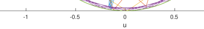
Figure 2.1: Phase plane plots for the second order harmonic oscillator model with $\omega=1$ and $\Delta t=3/2,\,1,\,1/2,\,1/10$

.

A natural proposal for a second-order accurate discrete conserved quantity is

$$C^{n}=(u^{n})^{2}+\left(\frac{u^{n+1}-u^{n-1}}{2\,\omega\,\Delta t}\right)^{2}\,.$$

A little algebra shows that $C^{n}$ is not conserved. However this computation shows that

$$C^{n}=\left(1-\left(\frac{\omega\,\Delta t}{2}\right)^{2}\right)(u^{n})^{2}+\left(\frac{u^{n+1}-u^{n-1}}{2\,\omega\,\Delta t}\right)^{2}$$

is conserved. Consequently for $0<\Delta t/\omega<2$ the discretization is stable. It is important that this constraint is less restrictive than requiring an accurate solution. Thus there seems to be no advantage to using a discretization that is stable for all $\Delta t$?

The initial condition $u^{1}=u(0)+\Delta t\,u^{\prime}(0)$ is only first order accurate but a Taylor series expansion can be used to make the order of accuracy higher:

$$u^{1} =u(0)+\Delta t\,u^{\prime}(0)+\frac{1}{2}\,\Delta t^{2}\,u^{\prime\prime}(0)+\frac{1}{6}\,\Delta t^{3}\,u^{\prime\prime\prime}(0)+\cdots$$

$$=u(0)+\Delta t\,u^{\prime}(0)-\frac{1}{2}\,\Delta t^{2}\,\omega^{2}\,u(0)-\frac{1}{6}\,\Delta t^{3}\,\omega^{2}\,u^{\prime}(0)+\cdots$$ (2.4)

The program Oscillator2ndOrder.m produced Figure 2.1, confirming that the algorithm is stable for $0<\Delta t/\omega<2$ and that $C^{n}$ is constant to less than one part in $10^{15}$.

2.3 Staggering the Time Discretization

A time staggered grid is used to discretize the first order system (2.1) which is given by a primal grid $t^{n}=n\,\Delta t$ and a dual grid $t^{n+1/2}=(n+1/2)\,\Delta t$, where $\Delta t>0$ and $0\leq n<\infty$ is an integer. The staggered or leapfrog discretization of the harmonic oscillator is then given by

$$\frac{u^{n+1}-u^{n}}{\Delta t}=\omega\,v^{n+1/2},\quad n\geq 0\,,\quad\frac{v^{n+1/2}-v^{n-1/2}}{\Delta t}=-\omega\,u^{n},\quad n\geq 1\,.$$ (2.5)

The minus sign can be put in either equation, but it is important to have an $\omega$ in both equations. As before, the initial conditions $u(0)$ and $u^{\prime}(0)$ are given and then $u^{0}=u(0)$ and

$$v^{1/2} =v\left(\frac{\Delta t}{2}\right)$$

$$=v(0)+\frac{\Delta t}{2}\,v^{\prime}(0)+\frac{1}{2}\,\left(\frac{\Delta t}{2}\right)^{2}\,v^{\prime\prime}(0)+\frac{1}{6}\,\left(\frac{\Delta t}{2}\right)^{3}\,v^{\prime\prime\prime}(0)+\cdots$$

$$=v(0)+\frac{\Delta t}{2}\,\omega\,u(0)+\frac{1}{2}\,\left(\frac{\Delta t}{2}\right)^{2}\,\omega^{2}\,v(0)+\frac{1}{6}\,\left(\frac{\Delta t}{2}\right)^{3}\,\omega^{3}\,u(0)+\cdots$$ (2.6)

The update algorithm starts with $u^{0}$ and $v^{1/2}$ and then for $n\geq 0$

$$u^{n+1}=u^{n}+\Delta t\,\omega\,v^{n+1/2}\,,\quad v^{n+3/2}=v^{n+1/2}-\Delta t\,\omega\,u^{n+1}\,.$$

Note that the second equation depends on the update in the first equation, so the order of evaluation is critical.

This staggered grid discretization gives two standard single grid discretization of the second order oscillator equation:

$$\frac{u^{n+2}-2\,u^{n+1}+u^{n}}{\Delta t^{2}}+\omega^{2}u^{n+1}=0\,;\quad\frac{v^{n+3/2}-2\,v^{n+1/2}+v^{n-1/2}}{\Delta t^{2}}+\omega^{2}v^{n+1/2}=0\,.$$

So the solution of the fractional step methods is identical to the solution of the second order equations.

Again a simple proposed conserved quantity for (2.5) is

$$C^{n}=\frac{1}{2}\left((u^{n})^{2}+\left(\frac{v^{n+1/2}+v^{n-1/2)}}{2}\right)^{2}\right)\,.$$ (2.7)

A little algebra gives

$$C^{n+1}-C^{n}=\frac{\omega^{2}\,\Delta t^{2}}{4}\,\left((u^{n+1})^{2}-(u^{n})^{2}\right)\,.$$

So $C^{n}$ is not conserved. However, set

$$\alpha=\frac{\omega\,\Delta t}{2}\,,$$

and then the following two quantities are conserved:

$$C^{n}=\frac{1}{2}\left(\left(1-\alpha^{2}\right)(u^{n})^{2}+\left(\frac{v^{n+1/2}+v^{n-1/2)}}{2}\right)^{2}\right)\,;$$ (2.8)

$$C^{n+1/2}=\frac{1}{2}\left(\left(\frac{u^{n+1}+u^{n}}{2}\right)^{2}+\left(1-\alpha^{2}\right)(v^{n+1/2})^{2}\right)\,.$$ (2.9)

The important properties for the staggered scheme are that it is explicit, second order accurate and stable for $\alpha=\omega\,\Delta t/2<1$. By modifying the discretization, a similar result was obtained in [47], Equation 45, for the Yee time discretization of Maxwell’s equations.

The code StaggeredOscillator.m confirms that the two energies are constant to one part in $10^{15}$. The phase plane plots for the staggered grid and the second order equation are identical. The code also estimates that for $\omega=1$, $\Delta t<2$ is required for stability, but for such a large $\Delta t$ the numerical solution is very inaccurate, as made clear in Figure 2.1. So the stability constraint on the time step is far less stringent than the accuracy constraint.

2.4 Summary

If conserved quantities for the harmonic oscillator are allowed to depend on $\Delta t$ then it is possible to derive conserved quantities that converge quadratically to the energy of the continuum differential equation. The restriction on $\Delta t$ to keep the conserved quantity positive is less stringent than the restriction for reasonably accurate solutions. All discretizations considered are confirmed to be second order accurate in using StaggeredOscillator.m. For generalizing these results to more complex wave equation it is important that there are no division by $\omega$ in the numerical algorithms.

3 Systems of Ordinary Differential Equations

The next task is to consider a special class of systems of linear ordinary differential equations that are wave equations. The discrete conservation laws are easy to find by following the harmonic oscillator example.

3.1 Continuous Time

Let $X$ and $Y$ be linear spaces (finite or infinite dimensional). It is important that it is not assumed that $X$ and $Y$ have the same dimension. If $f$ and $g$ are in $X$ then their inner product is $\langle f,g\rangle$ and the norm of $f$ is given by $\left|\left|f\right|\right|^{2}=\langle f,f\rangle$, with the same notation for $Y$. Let $A$ be a linear operator mapping $X$ to $Y$ with adjoint $A^{*}$, then

$$X\overset{A}{\rightarrow}Y\,,\quad Y\overset{A^{*}}{\rightarrow}X\,,$$

and if $f\in X$ and $g\in Y$ then

$$\langle A\,f,g\rangle=\langle f,A^{*}\,g\rangle\,.$$

Next, if $f=f(t)\in X$ and $g=g(t)\in Y$ then a generalization of the harmonic oscillator system is given by

$$f^{\prime}=A\,g\,,\quad g^{\prime}=-A^{*}\,f\,,$$ (3.1)

or in matrix form

$$\left[\begin{matrix}f^{\prime}\\ g^{\prime}\end{matrix}\right]=\left[\begin{matrix}0&A\\ -A^{*}&0\end{matrix}\right]\left[\begin{matrix}f\\ g\end{matrix}\right]\,.$$

Because the matrix

$$\left[\begin{matrix}0&A\\ -A^{*}&0\end{matrix}\right]$$

is skew adjoint, it must have purely imaginary spectra and the solutions of this system must be made up of waves and constant solutions. All solutions are bounded in $t$. Both $f$ and $g$ are solutions of second order linear wave equations:

$$f^{\prime\prime}+A^{*}\,Af=0\,;\quad g^{\prime\prime}+A\,A^{*}g\ =0.$$

There are three natural initial conditions: for the system specify $f(0)$ and $g(0)$; for the second order equation in $f$ specify, $f(0)$ and $f^{\prime}(0)$; and for the second order equation in $g$ specify, $g(0)$ and $g^{\prime}(0)$.

If the dimensions of $X$ and $Y$ are the same so that it make sense to assume that $A$ is invertible then the system 3.1 will have properties similar to the harmonic oscillator system (2.1) when $\omega>0$. The most interesting case is when the dimensions of the spaces are different which provides insight in to the discretization of the scalar and vector wave equation and also the Maxwell equations. Also the case when $A$ is self adjoint, $A^{*}=A$, provides insight into the discretization of Maxwell’s equations.

If $f\in X$ and $g\in Y$ then

$$\langle A^{*}\,Af,f\rangle= \langle Af,Af\rangle=\langle f,A^{*}\,Af\rangle\,$$

$$\langle A\,A^{*}g,g\rangle= \langle A^{*}g,A^{*}g\rangle=\langle g,A\,A^{*}g\rangle\,.$$

Consequently both $A\,A^{*}$ and $A^{*}\,A$ are self-adjoint positive operators, but they may not be positive definite. Also if $h\neq 0$ and $A\,h=0$ then $g(t)=t\,h$ is an unbounded solution of the second second order equation while if $A^{*}h=0$ then $f(t)=t\,h$ is an unbounded solution of the first second order equation. For this $f(t)$ the system becomes $h=A\,g(t)\,,\quad g^{\prime}(t)=0\,.$ So $g(t)=k$ a constant and then $\langle h,h\rangle=\langle h,A\,k\rangle=\langle A^{*}h,k\rangle=0$, that is $h=0$ and then $f(t)=0$ and $g(t)=k$ and $A\,k=0$. So the unbounded solution of the second order equation is not a solution of the system, an advantage of using the system. If $f$ and $g$ are vectors of the same length and $A$ is invertible then the system and second order equations are consistent.

There is also a problem with the initial conditions for the system and the second order equations. If $A$ is an $n$ by $m$ matrix, then $A^{*}$ is $m$ by $n$ matrix and consequently $A\,A^{*}$ is an $n$ by $n$ matrix and $A^{*}\,A$ is an $m$ by $m$ matrix. So the first of the second order equation needs $2\,n$ initial conditions, and the second of the second-order equations needs $2\,m$ initial conditions. The system needs $n+m$ initial conditions. However, for example, if one knows $f(t)$ then $g(t)$ can be found using simple integration and the initial condition for $g(t)$ and conversely for knowing $g(t)$. If $n=m$ then the number of initial conditions are the same for all three variants of the ordinary differential equations. The $n\neq m$ is far more analogous to the situation for the scalar and vector wave and Maxwell’s equations than the $n=m$ case.

3.2 Continuous Time Conserved Quantities

An important point here is that there is a conserved quantity that is not analogous to energy but implies that the energy is conserved. The fundamental conserved quantity is

$$C(t)=\frac{1}{2}\left(\left|\left|f(t)\right|\right|^{2}+\left|\left|g(t)\right|\right|^{2}\right)\,,$$

which is analogous to (2.2). Because

$$C^{\prime}(t)=\langle f^{\prime}(t),f(t)\rangle+\langle g^{\prime}(t),g(t)\rangle=\langle A\,g(t),f(t)\rangle+\langle-A^{*}f(t),g(t)\rangle=0\,,$$

this quantity is conserved.

For the second order equations, an analog of the total energy that is the sum of the kinetic plus the potential energy is given by

$$E(t) =\frac{1}{2}\left(\left|\left|f^{\prime}(t)\right|\right|^{2}+\left|\left|A^{*}\,f(t)\right|\right|^{2}\right)$$

$$=\frac{1}{2}\left(\left|\left|A\,g(t)\right|\right|^{2}+\left|\left|g^{\prime}(t)\right|\right|^{2}\right)$$

$$=\frac{1}{2}\left(\left|\left|f^{\prime}(t)\right|\right|^{2}+\left|\left|g^{\prime}(t)\right|\right|^{2}\right)\,,$$ (3.2)

and is conserved because if $f,g$ are a solutions of the system then so are $f^{\prime}$ and $g^{\prime}$. Note that the linearly growing solution has constant energy but $C(t)$ is unbounded. The $C(t$) type conserved quantities will used from now on.

3.3 Staggered Time Discretization

A second order centered leapfrog discretization for the first order system is

$$\frac{f^{n+1}-f^{n}}{\Delta t}=A\,g^{n+1/2}\,,\quad\frac{g^{n+1/2}-g^{n-1/2}}{\Delta t}=-A^{*}\,f^{n}\,.$$

Assuming that $f^{0}$ and $g^{1/2}$ are given then for $n\geq 0$ the leapfrog time stepping scheme is

$$f^{n+1}=f^{n}+\triangle t\,A\,g^{n+1/2}\,,\quad g^{n+3/2}=g^{n+1/2}-\triangle t\,A^{*}\,f^{n+1}\,.$$

Again that the order of evaluation is important.

The initial conditions for the discretized system require $f^{0}=f(0)$ and $g^{1/2}=g(\Delta t/2)$. If $g(0)$ and $g^{\prime}(0)$ are given then

$$g^{1/2}\approx g^{0}+\frac{\Delta t}{2}\,g^{\prime}(0)\,.$$

If $f(0)$ and $g(0)$ are given then

$$g^{1/2}\approx g^{0}+\frac{\Delta t}{2}\,g^{\prime}(0)=g^{0}-\frac{\Delta t}{2}\,A^{*}\,f^{0}\,.$$

If $f(0)$ and $f^{\prime}(0)$ are given, interchange $g$ and $f$ in the discretization. The estimates can be more made more accurate as was done in section 2.6.

Both $f$ and $g$ satisfy a second order difference equation:

$$\frac{f^{n+1}-2f^{n}+f^{n-1}}{\Delta t^{2}} =-A\,A^{*}f^{n}\,;$$

$$\frac{g^{n+3/2}-2g^{n+1/2}+g^{n-1/2}}{\Delta t^{2}} =-A^{*}\,A\,g^{n+1/2}\,.$$ (3.3)

Additionally a second order average is needed for computing conserved quantities:

$$\frac{f^{n+1}+2\,f^{n}+f^{n-1}}{4} =f^{n}-\frac{\Delta t^{2}}{4}A\,A^{*}f^{n}\,;$$

$$\frac{g^{n+3/2}+2\,g^{n1/2}+g^{n-1/2}}{4} =g^{n+1/2}-\frac{\Delta t^{2}}{4}A^{*}\,A\,g^{n+1/2}\,.$$ (3.4)

When comparing this discretization to the simple oscillator discretization it is important that $\omega>0$, while here the operators $A$ and $A^{*}$ may not be invertible which is typically the case when studying spatially dependent partial differential wave equations.

3.4 Discrete Time Conserved Quantities

To show that $A$ not being invertible is not serious problem a detailed derivation of the conservation laws that are analogs of (2.9) and (2.8) are given. Let

$$C_{1}^{n+1/2} =\left|\left|\frac{f^{n+1}+f^{n}}{2}\right|\right|^{2}\,,$$

$$C_{2}^{n+1/2} =\left|\left|g^{n+1/2}\right|\right|^{2}\,,$$

$$C_{3}^{n+1/2} =\Delta t^{2}\left|\left|A\,g^{n+1/2}\right|\right|^{2}\,.$$

As before compute:

$$C_{1}^{n+1/2}-C_{1}^{n-1/2} =\langle\frac{f^{n+1}+2\,f^{n}+f^{n-1}}{4},f^{n+1}-f^{n-1}\rangle$$

$$=\langle f^{n}-\frac{\Delta t^{2}}{4}A\,A^{*}f^{n},f^{n+1}-f^{n-1}\rangle\,;$$

$$C_{2}^{n+1/2}-C_{1}^{n-1/2} =\langle g^{n+1/2}+g^{n-1/2},g^{n+1/2}-g^{n-1/2}\rangle$$

$$=\langle g^{n+1/2}+g^{n-1/2},-\Delta t\,A^{*}f^{n}\rangle$$

$$=-\Delta t\,\langle A\,g^{n+1/2}+A\,g^{n-1/2},f^{n}\rangle$$

$$=-\Delta t\,\langle\frac{f^{n+1}-f^{n-1}}{\Delta t},f^{n}\rangle$$

$$=\langle-f^{n},f^{n+1}-f^{n-1}\rangle\,;$$

$$C_{3}^{n+1/2}-C_{1}^{n-1/2} =\Delta t^{2}\langle A\,g^{n+1/2}-A\,g^{n-1/2}\,,\,A\,g^{n+1/2}+A\,g^{n-1/2}\rangle$$

$$=\Delta t^{2}\langle A\left(g^{n+1/2}-g^{n+1/2}\right)\,,\,\frac{f^{n+1}-f^{n-1}}{\Delta t}\rangle$$

$$=\Delta t^{2}\langle-\Delta t\,A\,A^{*}f^{n}\,,\,\frac{f^{n+1}-f^{n-1}}{\Delta t}\rangle$$

$$=-\Delta t^{2}\langle A\,A^{*}f^{n}\,,\,f^{n+1}-f^{n-1}\rangle\,.$$

Consequently $C=C_{1}+C_{2}-C_{3}/4$ is a conserved quantity, that is

$$C^{n+1/2}=\left|\left|\frac{f^{n+1}+f^{n}}{2}\right|\right|^{2}+\left(1-\frac{\Delta t^{2}}{4}\left|\left|A\right|\right|^{2}\right)\left|\left|g^{n+1/2}\right|\right|^{2}\,.$$ (3.5)

is positive and constant for $\Delta t$ sufficiently small.

Next let

$$C_{1}^{n} =\left|\left|\frac{g^{n+1/2}+g^{n-1/2}}{2}\right|\right|^{2}\,,$$

$$C_{2}^{n} =\left|\left|f^{n}\right|\right|^{2}\,,$$

$$C_{3}^{n} =\Delta t^{2}\left|\left|A^{*}\,f^{n}\right|\right|^{2}\,.$$

$$C_{1}^{n+1}-C_{1}^{n} =\langle\frac{g^{n+3/2}+2\,g^{n1/2}+g^{n-1/2}}{4}\,,\,g^{n+3/2}-g^{n-1/2}\rangle$$

$$=\langle g^{n+1/2}-\frac{\Delta t^{2}}{4}A^{*}\,A\,g^{n+1/2}\,,\,g^{n+3/2}-g^{n-1/2}\rangle\,.$$

$$C_{2}^{n+1}-C_{2}^{n} =\langle f^{n+1}-f^{n}\,,\,f^{n+1}+f^{n}\rangle$$

$$=\langle\Delta t\,A\,g^{n+1/2}\,,\,f^{n+1}+f^{n}\rangle$$

$$=\Delta t\langle g^{n+1/2}\,,\,A^{*}f^{n+1}+A^{*}f^{n}\rangle$$

$$=\Delta t\langle g^{n+1/2}\,,\,-\frac{g^{n+3/2}-g^{n-1/2}}{\Delta t}\rangle$$

$$=\langle-g^{n+1/2}\,,\,g^{n+3/2}-g^{n-1/2}\rangle\,.$$

$$C_{3}^{n+1}-C_{3}^{n} =\Delta t^{2}\langle A^{*}f^{n+1}-A^{*}f^{n}\,,\,A^{*}f^{n+1}+A^{*}f^{n}\rangle$$

$$=\Delta t^{2}\langle A^{*}f^{n+1}-A^{*}f^{n}\,,\,\frac{g^{n+3/2}-g^{n-1/2}}{\Delta t}\rangle$$

$$=\Delta t^{2}\langle\Delta t\,A^{*}A\,g^{n+1/2}\,,\,\frac{g^{n+3/2}-g^{n-1/2}}{\Delta t}\rangle$$

$$=\Delta t^{2}\langle A^{*}A\,g^{n+1/2}\,,\,g^{n+3/2}-g^{n-1/2}\rangle\,.$$

Consequently $C^{n}=C_{1}^{n}+C_{2}^{n}-C_{3}^{n}/4$ is a conserved quantity, that is

$$\left|\left|C^{n}\right|\right|=\left(1-\frac{\Delta t^{2}}{4}\left|\left|A^{*}\right|\right|^{2}\right)\left|\left|f^{n}\right|\right|^{2}+\left|\left|\frac{g^{n+1/2}+g^{n-1/2}}{2}\right|\right|^{2}\,,$$ (3.6)

is positive and constant for $\Delta t$ sufficiently small.

The program SystemsODEs.m tests these conservation laws for $A$ a $2\times 3$ random matrix showing that the energies are constant with an error less that than one part in $10^{14}$.

4 Discretizing the 1D Wave Equation

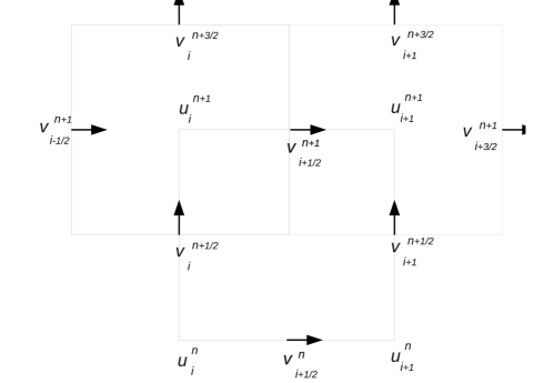
Figure 4.1: Space-Time Staggered Grid

The 1D scalar wave equation will be discretized by writing the equation as a system of two first order equations and then using a staggered time and spatial discretization. The time discretization is the same as leapfrog discretization used before while the spatial discretization is the mimetic discretization specialized to one dimension. Most importantly, a conserved quantity $C$ is introduced that is not the classical energy, but the conservation of $C$ implies the conservation of the energy $E$. This will play an important role in 3D discretizations.

Let $u=u(t,x)$ be a smooth real valued function of the real variables $x$ and $t$ such that $u(t,\pm\infty)=0$. Then let $u_{t}=\partial u/\partial t$, $u_{x}=\partial u/\partial x$, $u_{tt}=\partial^{2}u/\partial t^{2}$, and $u_{xx}=\partial^{2}u/\partial x^{2}$. The 1D wave equation is

$$u_{tt}=c^{2}\,u_{xx}\,,$$

where $c>0$. The initial conditions for this equation are $u(0,x)$ and $u_{t}(0,x)$.

This equation can also be written as a system

$$u_{t}=c\,v_{x}\,,\quad v_{t}=c\,u_{x}\,,$$ (4.1)

where again $v$ is smooth and $v(t,\pm\infty)=0$. The initial conditions are $u(0,x)$ and $v(0,x)$. As before $v$ also satisfies a second order wave equation

$$v_{tt}=c^{2}\,v_{xx}\,.$$

The vector spaces $X$ and $Y$ from Section 3 are replaced by $L^{2}$, the functions defined on the real line and are square integrable. The inner product of two functions $f=f(x)$ and $g=g(x)$ is

$$\langle f,g\rangle=\int_{-\infty}^{\infty}f(x)\,g(x)\,dx\,.$$

If $f(\pm\infty)=0$ and $g(\pm\infty)=0$ then integration by parts gives $\langle f^{\prime},g\rangle=\langle f,-g^{\prime}\rangle$, so if $A=\partial/\partial x$ then $-A^{*}=A$. So the wave equation has the has the same structure as the equations in the previous sections.

The usual energy $E=E(t)$ for the wave equation is the kinetic plus the potential energies,

$$E=\frac{1}{2}\int_{-\infty}^{\infty}\left(u_{t}^{2}+c^{2}\,u_{x}^{2}\right)dx\,.$$

Use integration by parts to see that

$$E_{t}= \int_{-\infty}^{\infty}\left(u_{t}\,u_{tt}+c^{2}\,u_{x}\,u_{tx}\right)\,dx\,.$$

$$= \int_{-\infty}^{\infty}\left(u_{t}\,u_{tt}-c^{2}\,u_{xx}u_{t}\right)\,dx=0\,,$$

that is, the energy $E(t)$ is conserved. As indicated in the previous sections a preferred conserved quantity is $C=C(t)$ where

$$C=\frac{1}{2}\int_{-\infty}^{\infty}\left(u^{2}+v^{2}\right)dx\,,$$ (4.2)

because

$$C_{t} =\int_{-\infty}^{\infty}\left(u\,u_{t}+v\,v_{t}\right)dx\,,$$

$$=\int_{-\infty}^{\infty}\left(u\,c\,v_{x}+v\,c\,u_{x}\right)dx\,,$$

$$=c\,\int_{-\infty}^{\infty}\left(u\,v_{x}+v\,u_{x}\right)dx\,,$$

$$=c\,\int_{-\infty}^{\infty}\left(u\,v\right)_{x}dx\,,$$

$$=0\,.$$

Again note that if $u,v$ are solutions of the system (4.1) then so are $u_{t}$, $v_{t}$ and then (4.2) implies that a conserved quantity is given by the energy

$$\frac{1}{2}\int_{-\infty}^{\infty}\left(u_{t}^{2}+v_{t}^{2}\right)dx=\frac{1}{2}\int_{-\infty}^{\infty}\left(u_{t}^{2}+c^{2}u_{x}^{2}\right)dx=E\,.$$

So if $C$ is conserved then so is $E$.

4.1 A Staggered Discretization of the Wave Equation

Let $\triangle t>0$ and $\triangle x>0$ be given and then the primal and dual grids points are given by

$$\left(t^{n},x_{i}\right)= \left(n\,\triangle t,i\,\triangle x\right)\,,$$

$$\left(t^{n+1/2},x_{i+1/2}\right)= \left((n+1/2)\,\triangle t,(i+1/2)\,\triangle x\right)\,,$$

where $-\infty<n<\infty$ and $-\infty<i<\infty$. The discretization of $u(x,t)$ on the primal grid and $v(x,t)$ on the dual grid are $u^{n}_{i}$ and $v^{n+1/2}_{i+1/2}$. Then the system (4.1) is discretized as

$$\frac{u^{n+1}_{i}-u^{n}_{i}}{\triangle t} =c\,\frac{v^{n+1/2}_{i+1/2}-v^{n+1/2}_{i-1/2}}{\triangle x}\,,$$

$$\frac{v^{n+1/2}_{i+1/2}-v^{n-1/2}_{i+1/2}}{\triangle t} =c\,\frac{u^{n}_{i+1}-u^{n}_{i}}{\triangle x}\,.$$ (4.3)

Assume that $u^{0}$ and $v^{{\frac{1}{2}}}$ are given then the leapfrog time stepping scheme for $n>0$ is

$$u^{n+1}_{i}=u^{n}_{i}+c\,\frac{\triangle t}{\triangle x}\left(v^{n+1/2}_{i+1/2}-v^{n+1/2}_{i-1/2}\right)\,,\quad v^{n+3/2}_{i+1/2}=v^{n+1/2}+c\,\frac{\triangle t}{\triangle x}\,\left(u^{n+1}_{i+1}-u^{n+1}_{i}\right)\,.$$

This implies that both $u$ and $v$ satisfy a discretization of the second order wave equation:

$$\frac{u^{n+1}_{i}-2\,u^{n}_{i}+u^{n-1}_{i}}{\triangle t^{2}} =\frac{1}{\triangle t}\left(\frac{u^{n+1}_{i}-\,u^{n}_{i}}{\triangle t}-\frac{u^{n}_{i}-u^{n-1}_{i}}{\triangle t}\right)$$

$$=\frac{c}{\triangle t}\left(\frac{v^{n+1/2}_{i+1/2}-v^{n+1/2}_{i-1/2}}{\triangle x}-\frac{v^{n-1/2}_{i+1/2}-v^{n-1/2}_{i-1/2}}{\triangle x}\right)$$

$$=\frac{c}{\triangle x}\left(\frac{v^{n+1/2}_{i+1/2}-v^{n-1/2}_{i+1/2}}{\triangle t}-\frac{v^{n+1/2}_{i-1/2}-v^{n-1/2}_{i-1/2}}{\triangle t}\right)$$

$$=\frac{c^{2}}{\triangle x}\left(\frac{u^{n}_{i+1}-u^{n}_{i}}{\triangle x}-\frac{u^{n}_{i}-u^{n}_{i-1}}{\triangle x}\right)$$

$$=c^{2}\,\frac{u^{n}_{i+1}-2\,u^{n}_{i}+u^{n}_{i-1}}{\triangle x^{2}}\,.$$

A similar calculation shows that

$$\frac{v^{n+1/2}_{i-1/2}-2\,v^{n-1/2}_{i-1/2}+v^{n-3/2}_{i-1/2}}{\triangle t^{2}}=c^{2}\,\frac{v^{n-1/2}_{i+1/2}-2\,v^{n-1/2}_{i-1/2}+v^{n-1/2}_{i-3/2}}{\triangle x^{2}}\,.$$

The inner product of two grid functions $a=(\cdots,a_{-1},a_{0},a_{1},\cdots)$ and $b=(\cdots,b_{-1},b_{0},b_{1},\cdots)$: is given by

$$\langle a,b\rangle=\sum_{i=-\infty}^{\infty}a_{i}\,b_{i}\,,\quad\left|\left|a\right|\right|^{2}=\langle a,a\rangle\,.$$

Similarly, if $c=(\cdots,c_{-1/2},c_{1/2},c_{3/2},\cdots)$ and $d=(\cdots,d_{-1/2},d_{1/2},d_{3/2},\cdots)$ then

$$\langle c,d\rangle=\sum_{i=-\infty}^{\infty}c_{i+1/2}\,d_{i+1/2}\,,\quad\left|\left|c\right|\right|^{2}=\langle c,c\rangle\,.$$

The discrete analogs of the integration by parts formula will be needed so let

$$\delta(a)_{i+1/2}=a_{i+1}-a_{i}\,,\quad\delta(c)_{i}=c_{i+1/2}-c_{i-1/2}\,.$$

Then the summation by parts formula is given by

$$\langle\delta(a),c\rangle =\sum_{i=-\infty}^{\infty}\left(a_{i+1}-a_{i}\right)c_{i+1/2}$$

$$=\sum_{i=-\infty}^{\infty}a_{i+1}c_{i+1/2}-\sum_{i=-\infty}^{\infty}a_{i}c_{i+1/2}$$

$$=\sum_{i=-\infty}^{\infty}a_{i}c_{i-1/2}-\sum_{i=-\infty}^{\infty}a_{i}c_{i+1/2}$$

$$=-\sum_{i=-\infty}^{\infty}a_{i}\left(c_{i+1/2}-c_{i-1/2}\right)$$

$$=-\langle a,\delta(c)\rangle\,.$$

The difference equations (4.1) can now be written

$$\frac{u^{n+1}_{i}-u^{n}_{i}}{\triangle t} =c\,\frac{\delta(v^{n+1/2})_{i}}{\triangle x}\,,$$

$$\frac{v^{n+1/2}_{i+1/2}-v^{n-1/2}_{i+1/2}}{\triangle t} =c\,\frac{\delta(u^{n})_{i+1/2}}{\triangle x}\,.$$ (4.4)

To find a conserved quantity define:

$$C1(n) =\left|\left|u^{n}\right|\right|^{2}\,;$$

$$C2(n) =\left|\left|\frac{v^{n+1/2}+v^{n-1/2}}{2}\right|\right|^{2}\,;$$

$$C3(n) =\left|\left|\delta(u^{n})\right|\right|^{2}\,.$$

Now

$$C1(n+1)-C1(n) =\langle u^{n+1}-u^{n},u^{n+1}+u^{n}\rangle$$

$$=c\,\frac{\triangle t}{\triangle x}\langle\delta(v^{n+1/2}),u^{n+1}+u^{n}\rangle\quad\text{see}\eqref{Vector Discretized System}$$

$$=c\,\frac{\triangle t}{\triangle x}\langle v^{n+1/2},-\delta(u^{n+1}+u^{n})\rangle$$

$$=-c\,\frac{\triangle t}{\triangle x}\langle v^{n+1/2},\delta(u^{n+1})+\delta(u^{n})\rangle$$

$$=-\langle v^{n+1/2},v^{n+3/2}-v^{n-1/2}\rangle\quad\text{see}\eqref{Vector Discretized System}\,.$$

$$C2(n+1)-C2(n) =\frac{1}{4}\langle v^{n+3/2}+v^{n+1/2}+v^{n+1/2}+v^{n-1/2},v^{n+3/2}+v^{n+1/2}-v^{n+1/2}-v^{n-1/2}\rangle$$

$$=\frac{1}{4}\langle v^{n+3/2}+2\,v^{n+1/2}+v^{n-1/2},v^{n+3/2}-v^{n-1/2}\rangle$$

$$=\langle v^{n+1/2},v^{n+3/2}-v^{n-1/2}\rangle+\frac{1}{4}\langle v^{n+3/2}-2\,v^{n+1/2}+v^{n-1/2},v^{n+3/2}-v^{n-1/2}\rangle$$

$$=\langle v^{n+1/2},v^{n+3/2}-v^{n-1/2}\rangle+c\,\frac{\triangle t}{4\,\triangle x}\langle\delta(u^{n+1})-\delta(u^{n}),v^{n+3/2}-v^{n-1/2}\rangle$$

$$=\langle v^{n+1/2},v^{n+3/2}-v^{n-1/2}\rangle+\left(c\,\frac{\triangle t}{2\,\triangle x}\right)^{2}\langle\delta(\delta(v^{n+1/2})),v^{n+3/2}-v^{n-1/2}\rangle$$

$$C3(n+1)-C3(n) =\langle\delta(u^{n+1})-\delta(u^{n}),\delta(u^{n+1})+\delta(u^{n})\rangle$$

$$=\langle\delta(u^{n+1}-u^{n}),\delta(u^{n+1})+\delta(u^{n})\rangle$$

$$=c\,\frac{\triangle x}{\triangle t}\langle\delta(u^{n+1})-\delta(u^{n}),v^{n+3/2}-v^{n-1/2}\rangle$$

$$=\langle\delta(\delta(v^{n+1/2})),v^{n+3/2}-v^{n-1/2}\rangle$$

Consequently the quantity

$$C(n)=\left|\left|u^{n}\right|\right|^{2}-\left(\frac{c\,\triangle t}{2\,\triangle x}\right)^{2}\left|\left|\delta u^{n}\right|\right|^{2}+\left|\left|\frac{v^{n+1/2}+v^{n-1/2}}{2}\right|\right|^{2}\,,$$

is conserved. A similar argument shows that

$$C(n+1/2)=\left|\left|v^{n+1/2}\right|\right|^{2}-\left(\frac{c\,\triangle t}{2\,\triangle x}\right)^{2}\left|\left|\delta\,v^{n+1/2}\right|\right|^{2}+\left|\left|\frac{u^{n+1}+u^{n}}{2}\right|\right|^{2}\,.$$

is a conserved quantity. The program OneDWave.m shows that the conserved quantities are constant to within an error of less than 10e-14.

The first conserved quantity will be positive provided that

$$\frac{c\,\triangle t}{2\,\triangle x}\frac{\left|\left|\delta u^{n}\right|\right|}{\left|\left|u^{n}\right|\right|}<1\,.$$

But

$$\frac{\left|\left|\delta u^{n}\right|\right|}{\left|\left|u^{n}\right|\right|}\leq\left|\left|\delta\right|\right|\,,$$

so the conserved quantity will be positive if

$$c\,\frac{\triangle t}{\triangle x}<\frac{2}{\left|\left|\delta\right|\right|}\,.$$

Because $\left|\left|\delta\right|\right|=2$ (see Normdelta.m) this is the Courant-Friedrichs-Lewy (CFL) condition for stability.

The program Wave1D.m shows that conservation errors are less than one part in $10^{15}$ and that the convergence rate is 2.

5 3D Wave Equations

quantity	units	name
$\vec{x}$	$d$	spatial position
$\vec{u}$	$d$	displacement
$\rho>0$	$1/d^{3}$	density
$\sigma$	$1/d^{2}$	stress
$e$	$1$	strain
$C$	$1/d^{2}$	elastic properties
$\lambda>0$	$1/d$	Lamé parameter
$\mu>0$	$1/d$	Lamé parameter
$K$	$1/d$	bulk modulus
$Pa$	$1/d$	Pascal

Table 5.1: Quantities and their spatial units.

The main interest is in three dimensional wave equations of which there are several variants. Here the material properties are assumed to be constant. What is important is the spatial dimension $d$ of the variables and operators, see table 5.1. The differential operators divergence ${\vec{\nabla}\boldsymbol{\cdot}}$, curl ${\vec{\nabla}\times}$ and gradient ${\vec{\nabla}}$ all have spatial dimension $1/d$. Many wave equations are derived from Newton’s laws and thus have the form

$$\rho\,\frac{d^{2}W}{dt^{2}}=\mathscr{A}\,W\,,$$ (5.1)

where $W=W(t,x,y,z)$ is a scalar or vector function, $\rho$ is the density of the material that the wave is traveling in and $\mathscr{A}$ is $\pm$ a constant times a second order differential operator. Because such equations are linear in $W$ the dimensions of $W$ are not important. So the spatial dimension of $\mathscr{A}$ must be the same as $\rho$. Consequently the dimensionless form of this wave equation is

$$\frac{d^{2}W}{dt^{2}}=\frac{1}{\rho}\mathscr{A}\,W\,.$$

The differential operators in the wave equations will be compositions of two of the operators divergence ${\vec{\nabla}\boldsymbol{\cdot}}$, curl ${\vec{\nabla}\times}$ and gradient ${\vec{\nabla}}$ and thus will have spatial dimension $1/d^{2}$.

A critical point about wave equations is that the operator $\mathscr{A}$ must be negative definite that is all eigen values of this operator are real and strictly less than zero. This will guarantee that the solutions are oscillatory. For constant material properties functions that are linear in time will be solutions of the second order equation. These solutions do not go to zero at large distance from the origin and so are theoretically not allowed but can still cause problems in simulations.

Inner products and norms of scalar functions are needed to describe the conservation laws for wave equations. So assume that the scalar and vector functions are smooth and converge rapidly to zero for large distances from the origin. If $f$ and $g$ are such scalar function then their inner product and norm are

$$\langle f,g\rangle=\int_{{}^{3}}f(x,y,z)\,g(x,y,z)\,dx\,dy\,dz\,,\quad\left|\left|f\right|\right|^{2}=\langle f,f\rangle\,,$$

while if $\vec{u}$ and $\vec{v}$ are smooth vector functions then their inner product and norm are given by

$$\langle\vec{u},\vec{v}\rangle=\int_{{}^{3}}\vec{u}(x,y,z)\boldsymbol{\cdot}\vec{v}(x,y,z)\,dx\,dy\,dz\,,\quad\left|\left|\vec{u}\right|\right|^{2}=\langle\vec{u},\vec{u}\rangle\,.$$

5.1 The Scalar Wave Equation

For example the scalar wave equation is given by

$$\frac{d^{2}f}{dt^{2}}=c^{2}\,{\vec{\nabla}\boldsymbol{\cdot}}\,{\vec{\nabla}}\,f\,,$$ (5.2)

where $f=f(x,y,z,t)$ is a dimensionless scalar and $c$ is the constant sound speed with spatial dimension $d$. Consequently this scalar wave equation is dimensionless. Note that the sound speed is given by

$$c^{2}=\frac{K}{\rho}\,,$$

where $K$ is the bulk modulus of the material the sound is traveling in.

To apply the stagged time discretization to second order wave equations they must be converted to a first order system. For the scalar wave equation introduce $\vec{v}={\vec{\nabla}}f$ to get

$$\frac{df}{dt}=c\,{\vec{\nabla}\boldsymbol{\cdot}}\vec{v}\,,\quad\frac{d\vec{v}}{dt}=c\,{\vec{\nabla}}f\,.$$ (5.3)

Putting a $c$ is each of the first oder equations makes them dimensionless. Note that $\vec{v}$ satisfies a simple vector wave equation

$$\frac{d^{2}\vec{v}}{dt^{2}}=c^{2}\,{\vec{\nabla}}\,{\vec{\nabla}\boldsymbol{\cdot}}\,\vec{v}\,.$$

Consequently solving the system will produce a solution to both the simple scalar and vector wave equations.

For the first order system the quantity

$$C=\frac{\left|\left|f\right|\right|^{2}+\left|\left|\vec{v}\right|\right|^{2}}{2}$$

is conserved because

$$\frac{dC}{dt} =\langle f,\frac{df}{dt}\rangle+\langle\vec{v},\frac{d\vec{v}}{dt}\rangle$$

$$=\langle f,c\,{\vec{\nabla}\boldsymbol{\cdot}}\vec{v}\rangle+\langle\vec{v},c\,{\vec{\nabla}}f\rangle$$

$$=c\,\langle f,{\vec{\nabla}\boldsymbol{\cdot}}\vec{v}\rangle-c\,\langle{\vec{\nabla}\boldsymbol{\cdot}}\vec{v},f\rangle$$

$$=0$$ (5.4)

Note that if $f$ and $\vec{v}$ are solutions of the system then so are $df/dt$ and $d\vec{v}/dt$. So the conservation $C$ implies the conservation $E$. In fact and time or spatial derivative of the solution of the wave equation is also a solution so there are infinitely many conserved quantities. Consequently

$$E=\left|\left|\frac{df}{dt}\right|\right|^{2}+\left|\left|\frac{d\vec{v}}{dt}\right|\right|^{2}=\left|\left|\frac{df}{dt}\right|\right|^{2}+c^{2}\,\left|\left|{\vec{\nabla}}f\right|\right|^{2}\,.$$

is conserved and is the energy for the scalar wave equation.

5.2 The Elastic Wave Equation

In the case that $W$ is a vector $\vec{v}$ there are only two second order differential operators that can be made from the gradient ${\vec{\nabla}}$, the divergence ${\vec{\nabla}\boldsymbol{\cdot}}$ and the curl ${\vec{\nabla}\times}$ which are ${\vec{\nabla}\times}{\vec{\nabla}\times}\vec{v}$ and ${\vec{\nabla}}{\vec{\nabla}\boldsymbol{\cdot}}\vec{v}$. So it is no surprise that the elastic wave equation [26] is made up of these operators:

$$\rho\,\frac{d^{2}\vec{v}}{dt^{2}}=(\lambda+2\,\mu){\vec{\nabla}}{\vec{\nabla}\boldsymbol{\cdot}}\vec{v}-\mu{\vec{\nabla}\times}{\vec{\nabla}\times}\vec{v}\,,$$ (5.5)

where $\mu$ and $\lambda$ are constant scalars with spatial dimension $1/d$. Note that $\mu=0$ produces

$$\frac{d^{2}\vec{v}}{dt^{2}}=\frac{\lambda}{\rho}{\vec{\nabla}}{\vec{\nabla}\boldsymbol{\cdot}}\vec{v}\,,$$ (5.6)

which is the dimensionless simple vector wave equation.

If

$$a=\sqrt{\frac{(\lambda+2\,\mu)}{\rho}}\,,\quad b=\sqrt{\frac{\mu}{\rho}}$$

then, like for $c$ in the scalar wave equation, $a$ and $b$ have units $d$, so the elastic wave equation 5.5 can be written in dimensionless form as:

$$\frac{d^{2}\vec{v}}{dt^{2}}=a^{2}{\vec{\nabla}}{\vec{\nabla}\boldsymbol{\cdot}}\vec{v}-b^{2}{\vec{\nabla}\times}{\vec{\nabla}\times}\vec{v}\,.$$ (5.7)

This equation can be converted to a system of three dimensionless first order equations:

$$\frac{dg}{dt} =a\,{\vec{\nabla}\boldsymbol{\cdot}}\vec{v}$$

$$\frac{d\vec{u}}{dt} =b\,{\vec{\nabla}\times}\vec{v}$$

$$\frac{d\vec{v}}{dt} =a\,{\vec{\nabla}}g-b\,{\vec{\nabla}\times}\vec{u}\,.$$

The quantity

$$C=\frac{\left|\left|\vec{v}\right|\right|^{2}+\left|\left|\vec{u}\right|\right|^{2}+\left|\left|g\right|\right|^{2}}{2}\\ ,$$

is conserved because

$$\frac{dC}{dt} =\langle\frac{d\vec{v}}{dt},\vec{v}\rangle+\langle\frac{d\vec{u}}{dt},\vec{u}\rangle+\langle\frac{d\vec{g}}{dt},\vec{g}\rangle$$

$$=\langle a\,{\vec{\nabla}}g-b\,{\vec{\nabla}\times}\vec{u},\vec{v}\rangle+\langle b\,{\vec{\nabla}\times}\vec{v},\vec{u}\rangle+\langle a\,{\vec{\nabla}\boldsymbol{\cdot}}\vec{v},\vec{g}\rangle$$

$$=a\,\langle{\vec{\nabla}}g,\vec{v}\rangle-b\,\langle{\vec{\nabla}\times}\vec{u},\vec{v}\rangle+b\,\langle{\vec{\nabla}\times}\vec{v},\vec{u}\rangle+a\,\langle{\vec{\nabla}\boldsymbol{\cdot}}\vec{v},\vec{g}\rangle$$

$$=-a\,\langle g,{\vec{\nabla}\boldsymbol{\cdot}}\vec{v}\rangle-b\,\langle\vec{u},{\vec{\nabla}\times}\vec{v}\rangle+b\,\langle{\vec{\nabla}\times}\vec{v},\vec{u}\rangle+a\,\langle{\vec{\nabla}\boldsymbol{\cdot}}\vec{v},\vec{g}\rangle$$

$$=0$$

5.3 Maxwell Equations

quantity	units	name
$\vec{E}$	$1/d$	electric field
$\epsilon$	$1/d$	permeability tensor
$\vec{D}$	$1/d^{2}$	electric displacement
$\vec{H}$	$1/d$	magnetic field
$\mu$	$1/d$	permittivity tensor
$\vec{B}$	$1/d^{2}$	magnetic flux
${\vec{\nabla}\times}$	$1/d$	curl operator
${\vec{\nabla}\times}$	$1/d$	curl operator
$\vec{J}$	$1/d^{2}$	current

Table 5.2: Quantities and their units in the Maxwell equations [11].

The Maxwell Equations

$$\frac{d\vec{B}}{dt}+{\vec{\nabla}\times}\vec{E}=0\,,\quad\frac{d\vec{D}}{dt}-{\vec{\nabla}\times}\vec{H}={\vec{J}}\,.$$ (5.8)

$$\vec{B}=\mu\,\vec{H}\,,\quad\vec{D}=\epsilon\,\vec{E}\,.$$

provide an example that was studied by Yee [57] with essentially the same ideas that are used in this paper. Here $\vec{B}$, $\vec{E}$, $\vec{D}$ and $\vec{H}$ are vector functions of $(x,y,z,t)$ while $\mu$ and $\epsilon$ are symmetric positive definite matrices that depend only on the spatial variables. The meaning of variables and their distance units are given in Table 5.2. The Maxwell equations are a bit different in that they start as a first order system.

Eliminate $\vec{B}$ and $\vec{D}$ from the equation to get

$$\frac{d\vec{E}}{dt}=\epsilon^{-1}{\vec{\nabla}\times}\vec{H}\,,\quad\frac{d\vec{H}}{dt}=-\mu^{-1}{\vec{\nabla}\times}\vec{E}\,,$$ (5.9)

which is a dimensionless system. This system can be written as either of two dimensionless second order equations:

$$\frac{d^{2}\vec{E}}{dt^{2}}=-\epsilon^{-1}{\vec{\nabla}\times}\mu^{-1}{\vec{\nabla}\times}\vec{E}\,,\quad\frac{d^{2}\vec{H}}{dt^{2}}=-\mu^{-1}{\vec{\nabla}\times}\epsilon^{-1}{\vec{\nabla}\times}\vec{H}\,.$$ (5.10)

Because $\epsilon$ and $\mu$ are matrices and not numbers the conserved quantity must be changed a bit:

$$C=\frac{\langle\epsilon\vec{E},\vec{E}\rangle+\langle\mu\vec{H},\vec{H}\rangle}{2}\\$$ (5.11)

Because $\epsilon$ and $\mu$ are symmetric matrices

$$\frac{dC}{dt} =\langle\epsilon\frac{d\vec{E}}{dt},\vec{E}\rangle+\langle\mu\frac{d\vec{H}}{dt},\vec{H}\rangle$$

$$=\langle{\vec{\nabla}\times}\vec{H},\vec{E}\rangle-\langle{\vec{\nabla}\times}\vec{E},\vec{H}\rangle$$

$$=\langle\vec{H},{\vec{\nabla}\times}\vec{E}\rangle-\langle{\vec{\nabla}\times}\vec{E},\vec{H}\rangle$$

$$=0$$ (5.12)

The vector identity

$${\vec{\nabla}}\boldsymbol{\cdot}(\vec{E}\times\vec{H})=({\vec{\nabla}\times}\vec{E})\boldsymbol{\cdot}\vec{H}-\vec{E}\boldsymbol{\cdot}({\vec{\nabla}\times}\vec{H})\,.$$

can also be used to see that the energy is constant. The time derivative of $C$ can be written using integrals as

$$\frac{dC}{dt} =\int_{{}^{3}}\left(\epsilon\,\frac{d\vec{E}}{dt}\boldsymbol{\cdot}\vec{E}+\mu\,\frac{\vec{H}}{dt}\boldsymbol{\cdot}\vec{H}\right)\,dx\,dy\,dz\,,$$

$$=\int_{{}^{3}}\left({\vec{\nabla}\times}\vec{H}\boldsymbol{\cdot}\vec{E}-{\vec{\nabla}\times}\vec{E}\boldsymbol{\cdot}\vec{H}\right)\,dx\,dy\,dz\,,$$

$$=-\int_{{}^{3}}{\vec{\nabla}\boldsymbol{\cdot}}(\vec{H}\times\vec{E})\,dx\,dy\,dz\,,$$

$$=\int_{{}^{3}}{\vec{\nabla}\boldsymbol{\cdot}}(\vec{E}\times\vec{H})\,dx\,dy\,dz\,,$$

$$=\int_{{}^{3}}{\vec{\nabla}\boldsymbol{\cdot}}\vec{S}\,dx\,dy\,dz\,,$$

$$=0\,.$$

The last integral is zero because it was assumed that $\vec{E}$ and $\vec{H}$ are zero far from the origin. Also $\vec{S}=\vec{E}\times\vec{H}$ is called the Poynting vector which has spatial units $1/d^{2}$. The integrand is the standard energy density confirming $C$ is spatially dimensionless.

6 Variable Coefficient Differential Operators

The first task is to describe all second order operators with variable coefficients that can be generated using diagram chasing in the double exact sequence shown in Figure 6.1. Next inner products are introduced on the $H$ spaces and the adjoints of all of the operators in the double exact sequence are computed. This is then used to show that the second order operators are self-adjoint and either positive or negative. The second order operators and the adjoint operators can be found quickly by diagram chasing as will be described. In the continuum setting there are two equivalent derivations of each operator. In the discrete setting these will be different.

6.1 Exact Sequences

$$\setcounter{MaxMatrixCols}{11}\begin{CD}{\genfrac{}{}{0.0pt}{}{0}{H_{P}}}@>{{\vec{\nabla}}}>{}>{\genfrac{}{}{0.0pt}{}{1}{H_{C}}}@>{{\vec{\nabla}\times}}>{}>{\genfrac{}{}{0.0pt}{}{2}{H_{S}}}@>{{\vec{\nabla}\boldsymbol{\cdot}}}>{}>{\genfrac{}{}{0.0pt}{}{3}{H_{V}}}\\ @V{a}V{}V@V{{\bf A}}V{}V@A{}A{{\bf B}}A@A{}A{b}A\\ {\genfrac{}{}{0.0pt}{}{H_{V}}{3}}@<{{\vec{\nabla}\boldsymbol{\cdot}}}<{}<{\genfrac{}{}{0.0pt}{}{H_{S}}{2}}@<{{\vec{\nabla}\times}}<{}<{\genfrac{}{}{0.0pt}{}{H_{C}}{1}}@<{{\vec{\nabla}}}<{}<{\genfrac{}{}{0.0pt}{}{H_{P}}{0}}\\ \end{CD}$$

Figure 6.1: Continuum Double Exact Sequence Diagram

In the double exact sequence diagram 6.1 the bottom row is the same as the top row written in opposite order. For reasons which will become clear when the operators are discretized, $P$ stands for points, $C$ stands for curves, $S$ stands for surfaces, $V$ stands for volumes. In this diagram $H_{P}$ and $H_{V}$ are linear spaces of smooth scalar functions depending on the spatial variables $(x,y,z)$ and $H_{C}$ and $H_{S}$ are linear spaces of smooth vector functions that depend also on $(x,y,z)$. All of the functions converge rapidly to zero as $x^{2}+y^{2}+z^{2}$ becomes large. The first order differential operators are the gradient ${\vec{\nabla}}$, curl or rotation ${\vec{\nabla}\times}$, and divergence ${\vec{\nabla}\boldsymbol{\cdot}}$. The scalar functions $a$ and $b$ and also the matrix valued functions ${\bf A}$ and ${\bf B}$ are also smooth function of the spatial variables that are used to describe material properties. The functions $a$ and $b$ are bounded above and below by positive constants. The matrix functions are symmetric positive definite and the eigenvalues of the matrices are bound above and below by positive constants.

$\text{if }f\in H_{P}$ $\text{ then }{\vec{\nabla}}f\in H_{C}$	$\text{if }f\in H_{P}$ $\text{ then }a\,f\in H_{V}$
$\text{if }\vec{v}\in H_{C}$ $\text{ then }{\vec{\nabla}\times}\vec{v}\in H_{S}$	$\text{if }\vec{v}\in H_{C}$ $\text{ then }{\bf A}\,\vec{v}\in H_{S}$
$\text{if }\vec{w}\in H_{S}$ $\text{ then }{\vec{\nabla}\boldsymbol{\cdot}}\vec{w}\in H_{V}$	$\text{if }\vec{w}\in H_{C}$ $\text{ then }{\bf B}\,\vec{w}\in H_{S}$
	$\text{if }g\in H_{P}$ $\text{ then }b\,g\in H_{V}$

Table 6.1: First order operators on the left, material property operators on the right.

The differential operators and material property functions give mappings between the spaces in the double exact sequence as described in Table 6.1. Note that the differential operators are not invertible, but that the conditions on the material properties function imply that they give invertible mappings. The horizontal arrows represent the action of the differential operators while the vertical arrows represent multiplication by scalar functions $a$ and $b$ and by $3\times 3$ matrices ${\bf A}$ and ${\bf B}$ that are known as star operators in differential geometry. The directions of the vertical arrows in the double exact sequence can be chosen to be either up or down as the operators are invertible.

The integers in the double exact sequence give the spatial dimension of the function in the spaces, that is if $f\in H_{P}$ the $f$ has no spatial dimension while if $g\in H_{V}$ then $g$ has spatial dimension $1/d^{3}$. Also if $\vec{v}\in H_{C}$ then $\vec{v}$ has spatial dimension $1/d$ and if $\vec{w}\in H_{S}$ then $\vec{w}$ has spatial dimension $1/d^{2}$. The differential operators all have dimension $1/d$. Moreover $a$ and $b$ have spatial dimensions $1/d^{3}$ while $\bf A$ and $\bf B$ have dimensions $1/d$. The directions of the vertical arrows were chosen so that $a$, $b$, $\bf A$ and $\bf B$ had dimensions $1/d^{k}$ for $k>0$.

Importantly, all of the operators given Table 6.1 are dimensionally consistent and all of the spaces in the double exact sequence

The most important properties of exactness are that ${\vec{\nabla}\boldsymbol{\cdot}}\,{\vec{\nabla}\times}=0$ and ${\vec{\nabla}\times}\,{\vec{\nabla}}=0$. Discretization that violate either of these two conditions are not mimetic! Additionally, exactness requires the existence of local scalar and vector potentials. That is, if $\vec{v}\in H_{C}$ and ${\vec{\nabla}\times}\vec{v}=0$ then there an $f\in H_{P}$ so that ${\vec{\nabla}}f=\vec{v}$ and if $\vec{w}\in H_{S}$ and ${\vec{\nabla}\boldsymbol{\cdot}}\vec{w}=0$ then there is an $\vec{v}\in H_{C}$ so that $\vec{w}={\vec{\nabla}\times}\vec{v}$.

6.2 Diagram Chasing and Second Order Operators

Upper Row		Bottom Row
First Box
$f\in H_{P}$	$\vec{v}\in H_{C}$	$\vec{w}\in H_{S}$	$g\in H_{V}$
${\vec{\nabla}}f\in H_{C}$	${\bf A}\vec{v}\in H_{S}$	${\vec{\nabla}\boldsymbol{\cdot}}\vec{w}\in H_{V}$	$a^{-1}g\in H_{P}$
${\bf A}{\vec{\nabla}}f\in H_{S}$	${\vec{\nabla}\boldsymbol{\cdot}}{\bf A}\vec{v}\in H_{V}$	$a^{-1}{\vec{\nabla}\boldsymbol{\cdot}}\vec{w}\in H_{P}$	${\vec{\nabla}}a^{-1}g\in H_{C}$
${\vec{\nabla}\boldsymbol{\cdot}}{\bf A}{\vec{\nabla}}f\in H_{V}$	$a^{-1}{\vec{\nabla}\boldsymbol{\cdot}}{\bf A}\vec{v}\in H_{P}$	${\vec{\nabla}}a^{-1}{\vec{\nabla}\boldsymbol{\cdot}}\vec{w}\in H_{C}$	${\bf A}{\vec{\nabla}}a^{-1}g\in H_{S}$
$a^{-1}{\vec{\nabla}\boldsymbol{\cdot}}{\bf A}{\vec{\nabla}}f\in H_{P}$	${\vec{\nabla}}a^{-1}{\vec{\nabla}\boldsymbol{\cdot}}{\bf A}\vec{v}\in H_{C}$	${\bf A}{\vec{\nabla}}a^{-1}{\vec{\nabla}\boldsymbol{\cdot}}\vec{w}\in H_{S}$	${\vec{\nabla}\boldsymbol{\cdot}}{\bf A}{\vec{\nabla}}a^{-1}g\in H_{V}$
Second Box
$\vec{v}\in H_{C}$	$\vec{w}\in H_{S}$	$\vec{v}\in H_{C}$	$\vec{w}\in H_{S}$
${\vec{\nabla}\times}\vec{v}\in H_{S}$	${\bf B}^{-1}\vec{w}\in H_{C}$	${\vec{\nabla}\times}\vec{v}\in H_{S}$	${\bf A}^{-1}\vec{w}\in H_{C}$
${\bf B}^{-1}{\vec{\nabla}\times}\vec{v}\in H_{C}$	${\vec{\nabla}\times}{\bf B}^{-1}\vec{w}\in H_{S}$	${\bf A}^{-1}{\vec{\nabla}\times}\vec{v}\in H_{C}$	${\vec{\nabla}\times}{\bf A}^{-1}\vec{w}\in H_{S}$
${\vec{\nabla}\times}{\bf B}^{-1}{\vec{\nabla}\times}\vec{v}\in H_{S}$	${\bf A}^{-1}{\vec{\nabla}\times}{\bf B}^{-1}\vec{w}\in H_{C}$	${\vec{\nabla}\times}{\bf A}^{-1}{\vec{\nabla}\times}\vec{v}\in H_{S}$	${\bf B}^{-1}{\vec{\nabla}\times}{\bf A}^{-1}\vec{w}\in H_{C}$
${\bf A}^{-1}{\vec{\nabla}\times}{\bf B}^{-1}{\vec{\nabla}\times}\vec{v}\in H_{C}$	${\vec{\nabla}\times}{\bf A}^{-1}{\vec{\nabla}\times}{\bf B}^{-1}\vec{w}\in H_{S}$	${\bf B}^{-1}{\vec{\nabla}\times}{\bf A}^{-1}{\vec{\nabla}\times}\vec{v}\in H_{C}$	${\vec{\nabla}\times}{\bf B}^{-1}{\vec{\nabla}\times}{\bf A}^{-1}\vec{w}\in H_{S}$
Third Box
$\vec{w}\in H_{S}$	$g\in H_{V}$	$f\in H_{P}$	$\vec{v}\in H_{C}$
${\vec{\nabla}\boldsymbol{\cdot}}\vec{w}\in H_{V}$	$b^{-1}g\in H_{P}$	${\vec{\nabla}}f\in H_{C}$	${\bf B}^{-1}\vec{v}\in H_{S}$
$b^{-1}{\vec{\nabla}\boldsymbol{\cdot}}\vec{w}\in H_{P}$	${\vec{\nabla}}{b^{-1}}g\in H_{C}$	${\bf B}{\vec{\nabla}}f\in H_{S}$	${\vec{\nabla}\boldsymbol{\cdot}}{\bf B}^{-1}\vec{v}\in H_{V}$
${\vec{\nabla}}b^{-1}{\vec{\nabla}\boldsymbol{\cdot}}\vec{w}\in H_{C}$	${\bf B}{\vec{\nabla}}b^{-1}g\in H_{S}$	${\vec{\nabla}\boldsymbol{\cdot}}{\bf B}{\vec{\nabla}}f\in H_{V}$	$b^{-1}{\vec{\nabla}\boldsymbol{\cdot}}{\bf B}^{-1}\vec{v}\in H_{P}$
${\bf B}{\vec{\nabla}}b^{-1}{\vec{\nabla}\boldsymbol{\cdot}}\vec{w}\in H_{S}$	${\vec{\nabla}\boldsymbol{\cdot}}{\bf B}{\vec{\nabla}}b^{-1}g\in H_{V}$	$b^{-1}{\vec{\nabla}\boldsymbol{\cdot}}{\bf B}{\vec{\nabla}}f\in H_{P}$	${\vec{\nabla}}b^{-1}{\vec{\nabla}\boldsymbol{\cdot}}{\bf B}^{-1}\vec{v}\in H_{C}$

Table 6.2: Fundamental second order differential operators. The left two columns start with spaces in the top row in Figure 6.1 while the right two columns start with spaces in the bottom row.

Table 6.2 gives all of the possible second order operators given by diagram chasing. As an example of diagram chasing, consider $f\in H_{P}$ so that ${\vec{\nabla}}f\in H_{C}$ and then ${\bf A}{\vec{\nabla}}f\in H_{S}$ so that ${\vec{\nabla}\boldsymbol{\cdot}}{\bf A}{\vec{\nabla}}f\in H_{V}$ and finally $a^{-1}{\vec{\nabla}\boldsymbol{\cdot}}{\bf A}{\vec{\nabla}}f\in H_{S}$. The gives the upper left entry in Table 6.2. The remaining operators are created similarly. For diagram chasing it is important that the mappings $a$, $b$, ${\bf A}$ and ${\bf B}$ are invertible while ${\vec{\nabla}}$, ${\vec{\nabla}\times}$ and ${\vec{\nabla}\boldsymbol{\cdot}}$ are not invertible. Consequently to create a second order operator, only going clockwise around a square in Figure 6.1 is allowed. However it is possible to start and any corner, so this gives twelve operators, four corners times three squares. In the continuum some of these operators are essentially the same, for example $a^{-1}{\vec{\nabla}\boldsymbol{\cdot}}{\bf A}{\vec{\nabla}}$ and $b^{-1}{\vec{\nabla}\boldsymbol{\cdot}}B{\vec{\nabla}}$. The assumption that ${\bf B}={\bf A}$ and $b=a$ reduces the number of operators to six. Finally, if $a=b=1$ and ${\bf A}={\bf B}=I$ the identity matrix then the operators simplify to those in Table 6.3 that is there are only three distinct second order operators:

$${\Delta}f={\vec{\nabla}\boldsymbol{\cdot}}{\vec{\nabla}}f\,;\quad\quad{\vec{\nabla}\times}{\vec{\nabla}\times}\vec{v}\,;\quad\quad{\vec{\nabla}}{\vec{\nabla}\boldsymbol{\cdot}}\vec{w}\,.$$

First Box
$f\in H_{P}$	$\vec{v}\in H_{C}$	$\vec{w}\in H_{S}$	$g\in H_{V}$
${\vec{\nabla}\boldsymbol{\cdot}}{\vec{\nabla}}f\in H_{P}$	${\vec{\nabla}}{\vec{\nabla}\boldsymbol{\cdot}}\vec{v}\in H_{C}$	${\vec{\nabla}}{\vec{\nabla}\boldsymbol{\cdot}}\vec{w}\in H_{S}$	${\vec{\nabla}\boldsymbol{\cdot}}{\vec{\nabla}}g\in H_{V}$
Second Box
$\vec{v}\in H_{C}$	$\vec{w}\in H_{S}$	$\vec{v}\in H_{C}$	$\vec{w}\in H_{S}$
${\vec{\nabla}\times}{\vec{\nabla}\times}\vec{v}\in H_{C}$	${\vec{\nabla}\times}{\vec{\nabla}\times}\vec{w}\in H_{S}$	${\vec{\nabla}\times}{\vec{\nabla}\times}\vec{v}\in H_{C}$	${\vec{\nabla}\times}{\vec{\nabla}\times}\vec{w}\in H_{S}$
Third Box
$\vec{w}\in H_{S}$	$g\in H_{V}$	$f\in H_{P}$	$\vec{v}\in H_{C}$
${\vec{\nabla}}{\vec{\nabla}\boldsymbol{\cdot}}\vec{w}\in H_{S}$	${\vec{\nabla}\boldsymbol{\cdot}}{\vec{\nabla}}g\in H_{V}$	${\vec{\nabla}\boldsymbol{\cdot}}{\vec{\nabla}}f\in H_{P}$	${\vec{\nabla}}{\vec{\nabla}\boldsymbol{\cdot}}\vec{v}\in H_{C}$

Table 6.3: The operators can be simplified by assuming that $a=b=1$ and that ${bfA}={\bf B}={\bf I}$, the identity matrix.

6.3 Additional Second Order Operators

Note that in Table 6.2 there are two operators defined on $H_{P}$, four operators defined on $H_{C}$, four operators defined on $H_{S}$ and two operators defined on $H_{V}$. If linear operators are defined on the same space then linear combinations of these operators are again linear operators. The two operators defined on $H_{P}$ and the two defined on $H_{V}$ are essentially the same so linear combinations are not interesting. For any operator in the Top Row boxes, there is a similar operator in the Bottom Row that can be obtained by interchanging $a$ with $b$ and ${\bf A}$ with ${\bf B}$. For $\vec{v}\in H_{C}$ and for $\vec{w}\in H_{S}$ define

$${\bf VL}_{1}(\vec{v}) ={\vec{\nabla}}a^{-1}\,{\vec{\nabla}\boldsymbol{\cdot}}\,{\bf A}\,\vec{v}-{\bf A}^{-1}\,{\vec{\nabla}\times}\,{\bf B}^{-1}\,{\vec{\nabla}\times}\,\vec{v}\,$$

$${\bf VL}_{2}(\vec{w}) ={\bf B}\,{\vec{\nabla}}b^{-1}\,{\vec{\nabla}\boldsymbol{\cdot}}\,\vec{w}-{\vec{\nabla}\times}\,{\bf A}^{-1}\,{\vec{\nabla}\times}\,{\bf B}^{-1}\,\vec{w}\,$$

$${\bf VL}_{3}(\vec{v}) ={\vec{\nabla}}\,b^{-1}\,{\vec{\nabla}\boldsymbol{\cdot}}\,{\bf B}\,\vec{v}-{\bf B}^{-1}\,{\vec{\nabla}\times}\,{\bf A}^{-1}\,{\vec{\nabla}\times}\,\vec{v}$$ (6.1)

$${\bf VL}_{4}(\vec{w}) ={\bf A}\,{\vec{\nabla}}\,a^{-1}\,{\vec{\nabla}\boldsymbol{\cdot}}\,\vec{w}-{\vec{\nabla}\times}\,{\bf B}^{-1}\,{\vec{\nabla}\times}\,{\bf A}^{-1}\,\vec{w}$$

Under the simplifying assumptions that $a=b=1$ and ${\bf A=\bf B=\bf I}$ these operators become

$${\mathbf{\Delta}}\vec{v}={\vec{\nabla}}{\vec{\nabla}\boldsymbol{\cdot}}\vec{v}-{\vec{\nabla}\times}{\vec{\nabla}\times}\vec{v}\,,\quad{\mathbf{\Delta}}\vec{w}={\vec{\nabla}}{\vec{\nabla}\boldsymbol{\cdot}}\vec{w}-{\vec{\nabla}\times}{\vec{\nabla}\times}\vec{w}\,,$$

which in Cartesian coordinates gives (see CurlCurl.nb) the vector Laplacian

$${\mathbf{\Delta}}\left(v_{1},v_{2},v_{3}\right)=\left({\Delta}v_{1},{\Delta}v_{2},{\Delta}v_{3}\right)\,,\quad{\mathbf{\Delta}}\left(w_{1},w_{2},w_{3}\right)=\left({\Delta}w_{1},{\Delta}w_{2},{\Delta}w_{3}\right)\,.$$

Operators like these appear in the elastic wave equation 5.5.

6.4 Inner Products

Applying the mimetic ideas to physical problems requires the use of inner products on the spaces $H_{P}$, $H_{C}$, $H_{S}$ and $H_{V}$. It is important that the inner products do not have a spatial dimension. Two bilinear forms will help simplify the notations. Let $f=f(x,y,z)\in H_{P}$,  $g=g(x,y,z)\in H_{V}$,  $\vec{v}=\vec{v(x,y,z)}\in H_{C}$ and $\vec{v}=\vec{w(x,y,z)}\in H_{S}$ and then define

$$\langle\langle f,g\rangle\rangle =\int_{{}^{3}}f(x,y,z)\,g(x,y,z)\,dx\,dy\,dz\,,$$

$$\langle\langle\vec{v},\vec{w}\rangle\rangle =\int_{{}^{3}}\vec{v}(x,y,z)\boldsymbol{\cdot}\vec{w}(x,y,z)\,dx\,dy\,dz\,.$$ (6.2)

These bilinear forms are dimensionless because $dx$, $dy$ and $dy$ have dimension $d$ while $f$ has dimension $0$, $g$ has dimension $1/d^{3}$, $\vec{v}$ has dimension $1/d$ and $\vec{w}$ has $1/d^{2}$.

The inner product on the function spaces must use a weight function to be dimensionless:

• for $f_{1}\,,f_{2}\in H_{P}$ set $\langle f_{1},f_{2}\rangle_{P}=\langle\langle a\,f_{1},f_{2}\rangle\rangle$

• for $\vec{v}_{1}\,,\vec{v}_{2}\in H_{C}$ set $\langle\vec{v}_{1},\vec{v}_{2}\rangle_{C}=\langle\langle{\bf A}\vec{v}_{1},\vec{v}_{2}\rangle\rangle$

• for $\vec{w}_{1}\,,\vec{w}_{2}\in H_{S}$ set $\langle\vec{w}_{1},\vec{w}_{2}\rangle_{S}=\langle\langle{\bf A}^{-1}\,\vec{w}_{1},\vec{w}_{2}\rangle\rangle$

• for $g_{1}\,,g_{2}\in H_{V}$ set $\langle g_{1},g_{2}\rangle_{V}=\langle\langle a^{-1}\,g_{1},g_{2}\rangle\rangle$

As usual $\left|\left|f\right|\right|_{P}^{2}=\langle f,f\rangle_{P}$, $\left|\left|\vec{v}\right|\right|_{C}^{2}=\langle\vec{v},\vec{v}\rangle_{C}$, $\left|\left|\vec{w}\right|\right|_{S}^{2}=\langle\vec{w},\vec{w}\rangle_{S}$, $\left|\left|g\right|\right|_{V}^{2}=\langle g,g\rangle_{V}$. Additional inner products can be made by replacing $a$ by $b$ and ${\bf A}$ by ${\bf B}$. To be inner products it is important that $a$ and $b$ are positive and that ${\bf A}$ and ${\bf B}$ are symmetric and positive definite matrices.

6.5 Adjoint Operators

Adjoints are commonly defined for operators mapping a space into itself but most of the operators used here are mapping between two different spaces, so the adjoint is defined as in Section 3.1. The discussion in that section shows that if $X$, $Y$, and $Z$ are linear spaces and $O_{1}$ and $O_{2}$ are linear operator such that:

$$X\overset{O_{1}}{\rightarrow}Y\overset{O_{2}}{\rightarrow}Z\quad\text{then }Z\overset{O_{2}^{*}}{\rightarrow}Y\overset{O_{1}^{*}}{\rightarrow}X\,$$

and

$$(O_{1}O_{2})^{*}=O_{2}^{*}\,O_{1}^{*}\,,\quad(O_{1}^{*})^{*}=O_{1}\,.$$

Because diagram chasing gives operators as compositions of other operators, this will be used many times.

The adjoints of the operators in Table 6.1 are

$${\vec{\nabla}}^{*} =-a^{-1}\,{\vec{\nabla}\boldsymbol{\cdot}}\,{\bf A} {\vec{\nabla}}^{*} =-b^{-1}\,{\vec{\nabla}\boldsymbol{\cdot}}\,{\bf B}\,,$$

$${\vec{\nabla}\times}^{*} =+{\bf A}^{-1}\,{\vec{\nabla}\times}\,{\bf B}^{-1} {\vec{\nabla}\times}^{*} =+{\bf B}^{-1}\,{\vec{\nabla}\times}\,{\bf A}^{-1}\,,$$

$${\vec{\nabla}\boldsymbol{\cdot}}^{*} =-{\bf B}{\vec{\nabla}}b^{-1} {\vec{\nabla}\boldsymbol{\cdot}}^{*} =-{\bf A}{\vec{\nabla}}a^{-1}\,,$$

$${\bf A}^{*} ={\bf A}^{-1} {\bf B}^{*} ={\bf B}^{-1}\,,$$ (6.3)

$$a^{*} =a^{-1} b^{*} =b^{-1}\,,$$

where the column on the left contains differential operators from the top row in Figure 6.1 and the column on the right contains differential operators from the bottom row in Figure 6.1.

Now the proofs of the formulas in 6.3 are straight forward. For the gradient let $f\in H_{P}$ and $\vec{v}\in H_{C}$ so that

$$\langle{\vec{\nabla}}f,\vec{v}\rangle_{C} =\langle\langle{\bf A}\,{\vec{\nabla}}f,\vec{v}\rangle\rangle$$

$$=\langle\langle{\vec{\nabla}}f,{\bf A}\,\vec{v}\rangle\rangle$$

$$=-\langle\langle f,{\vec{\nabla}\boldsymbol{\cdot}}\,{\bf A}\vec{v}\rangle\rangle$$

$$=-\langle\langle a\,f,a^{-1}\,{\vec{\nabla}\boldsymbol{\cdot}}\,{\bf A}\vec{v}\rangle\rangle$$

$$=\langle f,-a^{-1}\,{\vec{\nabla}\boldsymbol{\cdot}}\,{\bf A}\vec{v}\rangle_{P}$$

For the curl let $\vec{v}\in H_{C}$ and $\vec{w}\in H_{S}$ so that

$$\langle{\vec{\nabla}\times}\vec{v},\vec{w}\rangle_{S} =\langle\langle{\bf A}^{-1}\,{\vec{\nabla}\times}\vec{v},\vec{w}\rangle\rangle$$

$$=\langle\langle{\vec{\nabla}\times}\vec{v},{\bf A}^{-1}\,\vec{w}\rangle\rangle$$

$$=\langle\langle\vec{v},{\vec{\nabla}\times}\,{\bf A}^{-1}\vec{w}\rangle\rangle$$

$$=\langle\langle{\bf B}\,\vec{v},{\bf B}^{-1}\,{\vec{\nabla}\times}\,{\bf A}^{-1}\vec{v}\rangle\rangle$$

$$=\langle\vec{v},{\bf B}^{-1}\,{\vec{\nabla}\times}\,{\bf A}^{-1}\vec{w}\rangle_{C}$$

For the divergence let $\vec{w}\in H_{S}$ and $g\in H_{V}$ so that

$$\langle{\vec{\nabla}\boldsymbol{\cdot}}\vec{w},g\rangle_{V} =\langle\langle a^{-1}{\vec{\nabla}\boldsymbol{\cdot}}\vec{w},g\rangle\rangle$$

$$=\langle\langle{\vec{\nabla}\boldsymbol{\cdot}}\vec{w},a^{-1}g\rangle\rangle$$

$$=-\langle\langle\vec{w},{\vec{\nabla}}(a^{-1}g)\rangle\rangle$$

$$=-\langle\langle{\bf A}^{-1}\vec{w},{\bf A}{\vec{\nabla}}(a^{-1}g)\rangle\rangle$$

$$=\langle\vec{w},-{\bf A}{\vec{\nabla}}(a^{-1}g)\rangle_{S}$$

For the operator ${\bf A}$ let $\vec{v}\in H_{C}$ and $\vec{w}\in H_{S}$ so that

$$\langle{\bf A}\vec{v},\vec{w}\rangle_{S} =\langle\langle{\bf A}^{-1}{\bf A}\vec{v},\vec{w}\rangle\rangle$$

$$=\langle\langle{\bf A}\vec{v},{\bf A}^{-1}\vec{v}\rangle\rangle$$

$$=\langle\vec{v},{\bf A}^{-1}\vec{v}\rangle_{C}$$

For the operator $a$ let $f\in H_{P}$ and $g\in H_{V}$ so that

$$\langle a\,f,g\rangle_{V} =\langle\langle a^{-1}a\,f,g\rangle\rangle$$

$$=\langle\langle a\,f,a^{-1}g\rangle\rangle$$

$$=\langle f,a^{-1}g\rangle_{P}$$

Similar arguments give the adjoint operators for operators containing $b$ and ${\bf B}$. To keep the notation easy to read it has not been specified whether to use $a$ or $b$ and whether to use ${\bf A}$ or ${\bf B}$ in the inner products when computing adjoints. This is clear from the context.

It is now straight forward to compute the adjoints of the second order operators in Table 6.2:

$$\left(a^{-1}{\vec{\nabla}\boldsymbol{\cdot}}{\bf A}{\vec{\nabla}}\right)^{*} ={\vec{\nabla}}^{*}\,{\bf A}^{*}\,{\vec{\nabla}\boldsymbol{\cdot}}^{*}\,{a^{-1}}^{*}$$

$$=a^{-1}\,{\vec{\nabla}\boldsymbol{\cdot}}\,{\bf A}\,{\bf A}^{-1}\,{\bf A}\,{\vec{\nabla}}\,a^{-1}\,a$$ (6.4)

$$=a^{-1}\,{\vec{\nabla}\boldsymbol{\cdot}}\,{\bf A}\,{\vec{\nabla}}\,.$$

$$\left({\bf A}^{-1}\,{\vec{\nabla}\times}\,{\bf B}^{-1}\,{\vec{\nabla}\times}\,\right)^{*} ={\vec{\nabla}\times}^{*}\,{{\bf B}^{-1}}^{*}\,{\vec{\nabla}\times}^{*}\,{{\bf A}^{-1}}^{*}$$

$$={\bf A}^{-1}\,{\vec{\nabla}\times}\,{\bf B}^{-1}\,{\bf B}\,{\bf B}^{-1}\,{\vec{\nabla}\times}\,{\bf A}^{-1}\,{\bf A}$$ (6.5)

$$={\bf A}^{-1}\,{\vec{\nabla}\times}\,{\bf B}^{-1}\,{\vec{\nabla}\times}\,.$$

$$\left({\bf B}\,{\vec{\nabla}}b^{-1}\,{\vec{\nabla}\boldsymbol{\cdot}}\right)^{*} ={\vec{\nabla}\boldsymbol{\cdot}}^{*}\,{b^{-1}}^{*}\,{\vec{\nabla}}^{*}\,{\bf B}^{*}$$

$$={\bf B}\,{\vec{\nabla}}\,b^{-1}\,b\,b^{-1}\,{\vec{\nabla}\boldsymbol{\cdot}}\,{\bf B}\,{\bf B}^{-1}$$ (6.6)

$$={\bf B}\,{\vec{\nabla}}\,b^{-1}\,{\vec{\nabla}\boldsymbol{\cdot}}$$

So these three operators are self-adjoint and similar arguments show that all operators in Table 6.2 are self-adjoint.

6.6 Positive and Negative Second Order Operators

Arguments like those in the previous sections can be use to show that the second order operators in 6.2 are either positive or negative, those that contain two curl operators are positive while those that contain a gradient and divergence are negative.

Let $f\in H_{P}$ and then consider

$$\langle a^{-1}\,{\vec{\nabla}\boldsymbol{\cdot}}\,{\bf A}\,{\vec{\nabla}}\,f,f\rangle_{P} =\langle{\vec{\nabla}\boldsymbol{\cdot}}\,{\bf A}\,{\vec{\nabla}}\,f,a\,f\rangle_{V}$$

$$=-\langle{\bf A}\,{\vec{\nabla}}\,f,{\bf A}\,{\vec{\nabla}}\,a^{-1}\,a\,f\rangle_{S}$$

$$=-\langle{\bf A}\,{\vec{\nabla}}\,f,{\bf A}\,{\vec{\nabla}}\,f\rangle_{S}$$

$$\leq 0$$

Let $\vec{v}\in H_{C}$ and then consider

$$\langle{\bf A}^{-1}\,{\vec{\nabla}\times}\,{\bf B}^{-1}\,{\vec{\nabla}\times}\,\vec{v},\vec{v}\rangle_{C} =\langle{\vec{\nabla}\times}\,{\bf B}^{-1}\,{\vec{\nabla}\times}\,\vec{v},{\bf A}\,\vec{v}\rangle_{S}$$

$$=\langle{\bf B}^{-1}\,{\vec{\nabla}\times}\,\vec{v},{\bf B}^{-1}\,{\vec{\nabla}\times}\,{\bf A}^{-1}{\bf A}\vec{v}\rangle_{C}$$

$$=\langle{\bf B}^{-1}\,{\vec{\nabla}\times}\,\vec{v},{\bf B}^{-1}\,{\vec{\nabla}\times}\,\vec{v}\rangle_{C}$$

$$\geq 0$$

Let $\vec{w}\in H_{S}$ and then consider

$$\langle{\bf B}\,{\vec{\nabla}}b^{-1}\,{\vec{\nabla}\boldsymbol{\cdot}}\,\vec{w},\vec{w}\rangle_{S} =\langle{\vec{\nabla}}b^{-1}\,{\vec{\nabla}\boldsymbol{\cdot}}\,\vec{w},{\bf B}^{-1}\,\vec{w}\rangle_{S}$$

$$=\langle b^{-1}\,{\vec{\nabla}\boldsymbol{\cdot}}\,\vec{w},{\vec{\nabla}}^{*}\,{\bf B}^{-1}\,\vec{w}\rangle_{P}$$

$$=-\langle b^{-1}\,{\vec{\nabla}\boldsymbol{\cdot}}\,\vec{w},b^{-1}\,{\vec{\nabla}\boldsymbol{\cdot}}\,{\bf B}\,{\bf B}^{-1}\,\vec{w}\rangle_{P}$$

$$=-\langle b^{-1}\,{\vec{\nabla}\boldsymbol{\cdot}}\,\vec{w},b^{-1}\,{\vec{\nabla}\boldsymbol{\cdot}}\,\vec{w}\rangle_{P}$$

$$\leq 0$$

These results capture the important features of the homogeneous and isotropic second order differential operators.

7 Wave Equations With Variable Material Properties

This section describes all of the second order wave equations that can be generated using the operators that were generated using diagram chasing in Section 6. These wave equations have the form

$$\frac{d^{2}W}{dt^{2}}=\mathscr{A}\,W\,,$$

where $W=W(t,x,y,z)$ is a scalar or vector function and where $\mathscr{A}$ is $\pm$ an operator from Table 6.2 with the $+$ or $-$ chosen so that $\mathscr{A}$ is negative operator. This provides 12 possible wave equations. Another four equations are obtained using the operators in 6.1. Many of these equations are equivalent but will not be equivalent in the discrete setting. All of these equations are dimensionless as the map a space onto it self so the spatial dimensions of the functions play no role.

First six types of wave equations are introduced and then reduced to a easily recognized form for uniform material properties given by using the simplifying assumptions that $a=1/c^{3}$, $b=1/c^{3}$, ${\bf A}={\bf I}/c$ and ${\bf B}={\bf I}/c$. These assumptions keep the spatial dimensions correct.

Next first order systems are created using operators generate by going half way around the squares in the double exact sequence diagram 6.1. Note that these first order systems are not dimensionless because they map between space containing function with different spatial units. The first order systems are used to derived to create conservation laws for the first systems and consequently for the second order equations.

7.1 Scalar and Vector Wave Equations

To create a scalar wave equations choose $f=f(x,y,z,t)\in H_{P}$ and then define

$$\frac{d^{2}f}{dt^{2}}=a^{-1}{\vec{\nabla}\boldsymbol{\cdot}}{\bf A}{\vec{\nabla}}f\,.$$ (7.1)

Setting $f=a^{-1}\,g$ with $g\in H_{V}$ gives

$$\frac{d^{2}g}{dt^{2}}={\vec{\nabla}\boldsymbol{\cdot}}{\bf A}{\vec{\nabla}}a^{-1}g\,.$$ (7.2)

Under the simplifying assumptions these become the standard scalar wave equation

$$\frac{d^{2}f}{dt^{2}}=c^{2}\,{\vec{\nabla}\boldsymbol{\cdot}}\,{\vec{\nabla}}f\,,\quad\frac{d^{2}g}{dt^{2}}=c^{2}\,{\vec{\nabla}\boldsymbol{\cdot}}\,{\vec{\nabla}}g\,.$$

To create a vector wave equation choose $\vec{v}\in H_{C}$ to get

$$\frac{d^{2}\vec{v}}{dt^{2}}=-{\bf A}^{-1}\,{\vec{\nabla}\times}\,{\bf B}^{-1}\,{\vec{\nabla}\times}\,\vec{v}\,.$$ (7.3)

Setting $\vec{v}={\bf A}^{-1}\vec{w}$ with $\vec{w}\in H_{S}$ gives

$$\frac{d^{2}\vec{w}}{dt^{2}}=-{\vec{\nabla}\times}\,{\bf B}^{-1}\,{\vec{\nabla}\times}\,{\bf A}^{-1}\,\vec{w}\,.$$ (7.4)

Under the simplifying assumptions these become

$$\frac{d^{2}\vec{v}}{dt^{2}}=-c^{2}\,{\vec{\nabla}\times}\,{\vec{\nabla}\times}\,\vec{v}\,,\quad\frac{d^{2}\vec{w}}{dt^{2}}=-c^{2}\,{\vec{\nabla}\times}\,{\vec{\nabla}\times}\,\vec{w}\,,$$

which are Maxwell’s equations 5.8 in uniform materials.

More wave equations can be generated by choosing $\vec{w}\in H_{S}$:

$$\frac{d^{2}\vec{w}}{dt^{2}}={\bf B}\,{\vec{\nabla}}b^{-1}\,{\vec{\nabla}\boldsymbol{\cdot}}\,\vec{w}\,.$$ (7.5)

Setting $\vec{w}={\bf B}\,\vec{v}$ with $\vec{v}\in H_{C}$ gives

$$\frac{d^{2}\vec{v}}{dt^{2}}={\vec{\nabla}}\,b^{-1}\,{\vec{\nabla}\boldsymbol{\cdot}}\,{\bf B}\,\vec{v}\,.$$ (7.6)

Under the simplifying assumptions these become

$$\frac{d^{2}\vec{w}}{dt^{2}}=c^{2}\,{\vec{\nabla}}\,{\vec{\nabla}\boldsymbol{\cdot}}\,\vec{w}\,,\quad\frac{d^{2}\vec{v}}{dt^{2}}=c^{2}\,{\vec{\nabla}}\,{\vec{\nabla}\boldsymbol{\cdot}}\,\vec{v}\,.$$

In total twelve equations can be created offering useful flexibility in modeling physical problems.

Additional second order wave equations can be made from the two term second order operators ${\bf VL}_{1}$, ${\bf VL}_{2}$, ${\bf VL}_{3}$, and ${\bf VL}_{4}$ in 6.1. For example

$$\frac{d^{2}\vec{v}}{dt^{2}}={\vec{\nabla}}a^{-1}{\vec{\nabla}\boldsymbol{\cdot}}{\bf A}\vec{v}-{\bf A}^{-1}{\vec{\nabla}\times}{\bf B}^{-1}{\vec{\nabla}\times}\vec{v}\,.$$ (7.7)

To simplify this equation assume $a$ and $b$ are constants and ${\bf A}=a^{3}\,{\bf I}$ and ${\bf B}=1/(a^{3}\,b^{2}){\bf I}$ to get

$$\frac{d^{2}\vec{v}}{dt^{2}}=a^{2}\,{\vec{\nabla}}\,{\vec{\nabla}\boldsymbol{\cdot}}\,\vec{v}-b^{2}\,{\vec{\nabla}\times}\,{\vec{\nabla}\times}\vec{v}\,,$$

which is the elastic wave equation 5.7. All four equations created this way reduce to the elastic wave equation under simplifying assumptions.

7.2 First Order Systems and Conserved Quantities

There is a natural way to use diagram chasing to write the second order wave equations as a system and then use this to define a conserved quantity. Note that the first order equations are not dimensionless as in the constant coefficient case because the functions in the spaces the Continuum Double Exact Sequence Diagram 6.1 are not dimensionless. The main idea is two choose two function that in diagonally opposite corners of one of the squares in 6.1 and do a diagram chase. Consequently there are lots of first order systems!

For example for equation (7.1), because $f\in H_{P}$, choose $\vec{w}\in H_{S}$ and then set

$$\frac{d\vec{w}}{dt}={\bf A}{\vec{\nabla}}f\,,\quad\frac{df}{dt}=a^{-1}{\vec{\nabla}\boldsymbol{\cdot}}\,\vec{w}$$ (7.8)

Note that $\vec{w}$ also satisfies the second order vector wave equation (7.5) with ${\bf B}$ and $b$ replaced by ${\bf A}$ and $a$.

Table 6.3 implies that

$$(a^{-1}{\vec{\nabla}\boldsymbol{\cdot}})^{*}={\vec{\nabla}\boldsymbol{\cdot}}^{*}(a^{-1})^{*}=-A{\vec{\nabla}}a^{-1}a=-A{\vec{\nabla}}\,,$$

so this system has the form of the equation discussed in 3.1 and consequently should have a conserved quantity given by

$$C=\frac{\left|\left|f\right|\right|_{P}^{2}+\left|\left|\vec{w}\right|\right|_{S}^{2}}{2}$$

This can be checked explicitly:

$$\frac{dC}{dt} =\langle f,\frac{df}{dt}\rangle_{P}+\langle\vec{w},\frac{d\vec{w}}{dt}\rangle_{S}$$

$$=\langle f,a^{-1}{\vec{\nabla}\boldsymbol{\cdot}}\,\vec{w}\rangle_{P}+\langle\vec{w},{\bf A}{\vec{\nabla}}f\rangle_{S}$$

$$=\langle(a^{-1}{\vec{\nabla}\boldsymbol{\cdot}})^{*}f,\,\vec{w}\rangle_{S}+\langle\vec{w},{\bf A}{\vec{\nabla}}f\rangle_{S}$$

$$=-\langle{\bf A}\,{\vec{\nabla}}\,f,\vec{w}\rangle_{S}+\langle\vec{w},{\bf A}{\vec{\nabla}}f\rangle_{S}$$

$$=0$$

As discussed in Section 2 if $f$ and $\vec{w}$ are solutions of (7.8) then so are $df/dt$ and $d\vec{w}/dt$ and consequently the classical energy

$$E=\frac{\left|\left|\frac{df}{dt}\right|\right|_{P}^{2}+\left|\left|\frac{d\vec{w}}{dt}\right|\right|_{S}^{2}}{2}=\frac{\left|\left|\frac{df}{dt}\right|\right|_{P}^{2}+\left|\left|{\bf A}\,{\vec{\nabla}}f\right|\right|_{S}^{2}}{2}$$

is conserved.

For equation (7.2), because $g\in H_{V}$, choose $\vec{v}\in H_{C}$ and then set

$$\frac{d\vec{v}}{dt}={\vec{\nabla}}a^{-1}\,g\,,\quad\frac{dg}{dt}={\vec{\nabla}\boldsymbol{\cdot}}{\bf A}\,\vec{v}\,.$$ (7.9)

Again, with a change of notation this is (7.5). A conserved quantity is given by

$$C=\frac{\left|\left|g\right|\right|_{V}^{2}+\left|\left|\vec{v}\right|\right|_{C}^{2}}{2}$$

because

$$\frac{dC}{dt} =\langle g,\frac{dg}{dt}\rangle_{V}+\langle\vec{v},\frac{d\vec{v}}{dt}\rangle_{C}$$

$$=\langle g,{\vec{\nabla}\boldsymbol{\cdot}}{\bf A}\,\vec{v}\rangle_{V}+\langle\vec{v},{\vec{\nabla}}a^{-1}\,g\rangle_{C}$$

$$=\langle-{\bf A}^{-1}\,{\bf A}\,{\vec{\nabla}}\,a^{-1}\,g,\vec{v}\rangle_{C}+\langle\vec{v},{\vec{\nabla}}a^{-1}\,g\rangle_{C}$$

$$=-\langle{\vec{\nabla}}\,a^{-1}\,g,\vec{v}\rangle_{C}+\langle\vec{v},{\vec{\nabla}}a^{-1}\,g\rangle_{C}$$

$$=0$$

As before

$$E=\frac{\left|\left|\frac{dg}{dt}\right|\right|_{V}^{2}+\left|\left|\frac{d\vec{w}}{dt}\right|\right|_{S}^{2}}{2}=\frac{\left|\left|\frac{dg}{dt}\right|\right|_{V}^{2}+\left|\left|{\vec{\nabla}}\,a^{-1}g\right|\right|_{S}^{2}}{2}$$

is conserved.

For equation (7.3), because $\vec{v}\in H_{C}$, choose $\vec{u}\in H_{C}$ and then set

$$\frac{d\vec{u}}{dt}={\bf B}^{-1}\,{\vec{\nabla}\times}\,\vec{v}\,,\quad\frac{d\vec{v}}{dt}=-{\bf A}^{-1}\,{\vec{\nabla}\times}\,\vec{u}\,.$$

A conserved quantity is given by

$$C=\frac{\left|\left|\vec{v}\right|\right|_{C}^{2}+\left|\left|\vec{u}\right|\right|_{C}^{2}}{2}$$

because

$$\frac{dC}{dt} =\langle\vec{v},\frac{d\vec{v}}{dt}\rangle_{C}+\langle\vec{u},\frac{d\vec{u}}{dt}\rangle_{C}$$

$$=-\langle\vec{v},{\bf A}^{-1}\,{\vec{\nabla}\times}\,\vec{u}\rangle_{C}+\langle\vec{u},{\bf B}^{-1}\,{\vec{\nabla}\times}\,\vec{v}\rangle_{C}$$

$$=-\langle{\bf B}^{-1}{\vec{\nabla}\times}{\bf A}^{-1}\,{\bf A}\vec{v},\vec{u}\rangle_{C}+\langle\vec{u},{\bf B}^{-1}\,{\vec{\nabla}\times}\,\vec{v}\rangle_{C}$$

$$=-\langle{\bf B}^{-1}{\vec{\nabla}\times}\vec{v},\vec{u}\rangle_{C}+\langle\vec{u},{\bf B}^{-1}\,{\vec{\nabla}\times}\,\vec{v}\rangle_{C}$$

$$=0$$

Additionally,

$$E=\frac{\left|\left|\frac{d\vec{u}}{dt}\right|\right|_{C}^{2}+\left|\left|\frac{d\vec{v}}{dt}\right|\right|_{C}^{2}}{2}=\frac{\left|\left|{\bf B}^{-1}\,{\vec{\nabla}\times}\,\vec{v}\right|\right|_{C}^{2}+\left|\left|{\bf A}^{-1}\,{\vec{\nabla}\times}\,\vec{u}\right|\right|_{C}^{2}}{2}=\frac{\left|\left|{\vec{\nabla}\times}\,\vec{v}\right|\right|_{S}^{2}+\left|\left|{\vec{\nabla}\times}\,\vec{u}\right|\right|_{S}^{2}}{2}\,,$$

is a conserved quantity. In this case the first order system is essentially Maxwell’s equations and $C$ is essentially the physical energy.

For equation (7.4), because $\vec{v}\in H_{C}$, choose $\vec{u}\in H_{C}$ and then set

$$\frac{d\vec{u}}{dt}=-{\vec{\nabla}\times}\,{\bf A}^{-1}\,\vec{w}\,,\quad\frac{d\vec{v}}{dt}={\vec{\nabla}\times}\,{\bf B}^{-1}\,\vec{u}\,.$$

So $\vec{v}$ and $\vec{u}$ satisfy the previous first order system with $\vec{v}$ and $\vec{w}$ interchanged and thus has the same conserved quantity.

For equation (7.5), because $\vec{w}\in H_{S}$, choose $f\in H_{P}$ and then set

$$\frac{df}{dt}=b^{-1}\,{\vec{\nabla}\boldsymbol{\cdot}}\,\vec{w}\,,\quad\frac{d\vec{w}}{dt}={\bf B}\,{\vec{\nabla}}f\,.$$

Again $f$ satisfies (7.1) with $b$ and ${\bf B}$ replaced by $a$ and ${\bf A}$, so

$$C=\frac{\left|\left|\vec{w}\right|\right|_{C}^{2}+\left|\left|f\right|\right|_{P}^{2}}{2}$$

is conserved.

For equation (7.6), because $\vec{v}\in H_{C}$, choose $g\in H_{V}$ and then set

$$\frac{dg}{dt}={\vec{\nabla}\boldsymbol{\cdot}}\,{\bf B}\,\vec{v}\,,\quad\frac{d\vec{v}}{dt}={\vec{\nabla}}\,b^{-1}\,g\,.$$

Again $g$ satisfies (7.2) with $b$ and ${\bf B}$ replaced by $a$ and ${\bf A}$ so

$$C=\frac{\left|\left|\vec{v}\right|\right|_{C}^{2}+\left|\left|g\right|\right|_{V}^{2}}{2}$$

is conserved.

Also first order systems can be made from the second order equations made from the two term second order operators ${\bf VL}_{1}$, ${\bf VL}_{2}$, ${\bf VL}_{3}$ and ${\bf VL}_{4}$ given in 6.1. However this requires three first order equations. For example, for ${\bf VL}_{1}$, because $\vec{v}\in H_{C}$ let $g\in H_{V}$ and $\vec{u}\in H_{C}$ and then set

$$\frac{dg}{dt} ={\vec{\nabla}\boldsymbol{\cdot}}{\bf A}\vec{v}$$

$$\frac{d\vec{u}}{dt} ={\bf B}^{-1}{\vec{\nabla}\times}\vec{v}$$

$$\frac{d\vec{v}}{dt} ={\vec{\nabla}}a^{-1}g-{\bf A}^{-1}{\vec{\nabla}\times}\vec{u}\,.$$

For a conserved quantity set

$$C=\frac{\left|\left|\vec{v}\right|\right|_{C}^{2}+\left|\left|\vec{u}\right|\right|_{C}^{2}+\left|\left|g\right|\right|_{V}^{2}}{2}\\ ,$$

so that

$$\frac{dC}{dt} =\langle\vec{v}\,\frac{d\vec{v}}{dt}\rangle_{C}+\langle\vec{u}\,\frac{d\vec{u}}{dt}\rangle_{C}+\langle g\,\frac{dg}{dt}\rangle_{V}$$

$$=\langle\vec{v},{\vec{\nabla}}a^{-1}g-{\bf A}^{-1}{\vec{\nabla}\times}\vec{u}\rangle_{C}+\langle\vec{u},{\bf B}^{-1}{\vec{\nabla}\times}\vec{v}\rangle_{C}+\langle g,{\vec{\nabla}\boldsymbol{\cdot}}{\bf A}\vec{v}\rangle_{V}$$

$$=\langle\vec{v},{\vec{\nabla}}a^{-1}g\rangle-\langle\vec{v},{\bf A}^{-1}{\vec{\nabla}\times}\vec{u}\rangle_{C}+\langle{\bf A}^{-1}{\vec{\nabla}\times}{\bf B}^{-1}{\bf B}\vec{u},\vec{v}\rangle_{C}-\langle{\bf A}^{-1}{\bf A}{\vec{\nabla}}a^{-1}g,\vec{v}\rangle_{V}$$

$$=\langle\vec{v},{\vec{\nabla}}a^{-1}g\rangle-\langle\vec{v},{\bf A}^{-1}{\vec{\nabla}\times}\vec{u}\rangle_{C}+\langle{\bf A}^{-1}{\vec{\nabla}\times}\vec{u},\vec{v}\rangle_{C}-\langle{\vec{\nabla}}a^{-1}g,\vec{v}\rangle_{V}$$

$$=0\,.$$

As before this implies that

$$E =\frac{\left|\left|\frac{d\vec{v}}{dt}\right|\right|_{C}^{2}+\left|\left|\frac{d\vec{u}}{dt}\right|\right|_{C}^{2}+\left|\left|\frac{dg}{dt}\right|\right|_{V}^{2}}{2}$$

$$=\frac{\left|\left|\frac{d\vec{v}}{dt}\right|\right|_{C}^{2}+\left|\left|{\bf B}^{-1}{\vec{\nabla}\times}\vec{v}\right|\right|_{C}^{2}+\left|\left|{\vec{\nabla}\boldsymbol{\cdot}}{\bf A}\vec{v}\right|\right|_{V}^{2}}{2}$$

is conserved.

7.3 Examples

Maxwell equations for electrodynamics fit into the diagram chasing paradigm easily and will be discussed first. The general elastic wave equations are do not fit into the diagram chasing but many special cases of elastic or acoustic wave equations do fit well . The notation will be changed that used in the applications.

7.3.1 Maxwell’s Equation

$$\begin{CD}{\genfrac{}{}{0.0pt}{}{1}{H_{CU}}}@>{{\vec{\nabla}\times}}>{}>{\genfrac{}{}{0.0pt}{}{2}{H_{SU}}}\\ @V{\epsilon}V{}V@A{}A{\mu}A\\ {\genfrac{}{}{0.0pt}{}{H_{SD}}{2}}@<{{\vec{\nabla}\times}}<{}<{\genfrac{}{}{0.0pt}{}{H_{CD}}{1}}\\ \end{CD}$$

Figure 7.1: Maxwell Exact Sequences

Representing Maxwell’s equations 5.8 using diagram chasing uses the center square in Figure 6.1 which is reproduced in Figure 7.1 using notation appropriate to Maxwell’s equations, that is, by setting ${\bf A}=\epsilon$ and ${\bf B}=\mu$. Because in Figure 7.1 the upper left space and the lower right space have the same labels as well as the upper right space has the same label as as the lower left space they are relabeled with $U$ and $D$ standing for up and down, that is, as $H_{CU}$, $H_{CD}$, $H_{SU}$ and $H_{SD}$. Maxwell’s equations can be represented using $\vec{E}\in H_{CU}$, $\vec{H}\in H_{CD}$, $\vec{B}\in H_{SU}$ and $\vec{D}\in H_{SD}$. Here it is assumed that $\vec{J}=0$, but if this is not the case then $\vec{J}\in H_{SD}$.

To derive first order system of Maxwell’s equations by diagram chasing, start with $\vec{E}\in H_{CU}$ and then define $\vec{H}\in H_{CD}$ by

$$\frac{d\vec{H}}{dt}=-\mu^{-1}{\vec{\nabla}\times}\vec{E}\,,$$

and then introduce

$$\frac{d\vec{E}}{dt}=\epsilon^{-1}{\vec{\nabla}\times}\vec{H}\,.$$

The diagram chasing implies that a conserved quantity is given by

$$C=\frac{\langle\vec{E},\vec{E}\rangle_{CU}+\langle\vec{H},\vec{H}\rangle_{CD}}{2}\\$$ (7.10)

It is easy to check that this quantity is conserved and is the energy for the Maxwell equations, see Section 5.3.

7.3.2 General Elastic Wave Equations

This section is based on the discussion in [14] and a summary of the notation is given in Table 5.1. When there are no external forces the general elastic wave equation in a material with spatially variable properties is given by Newton’s law applied to the displacements of the material:

$$\rho\frac{d^{2}u_{i}}{dt^{2}}=\sum_{j=1}^{3}\frac{d{\sigma_{i,j}}}{d{x_{j}}}\,,\quad 1\leq i\leq 3$$ (7.11)

where $t$ is time, $\vec{u}=\vec{u}(\vec{x},t)$, are the displacements of the material, $\rho=\rho(\vec{x})$ is the density of the material, and $\sigma=\sigma(\vec{x})$ is the symmetric stress tensor:

$$\sigma_{i,j}=\sum_{k,l=1}^{3}C_{k,l,i,j}\,e_{k,l}\,.$$

This equation has the same form as the general wave equation in 5.1. The strains are

$$e_{i,j}=\frac{1}{2}\left(\frac{\partial u_{i}}{\partial x_{j}}+\frac{\partial u_{j}}{\partial x_{i}}\right)$$

which are dimensionless. The material properties other than density are given by the $C_{k,l,i,j}$ where $C=C(\vec{x})$ and where $C$ has the symmetries $C_{k,l,i,j}=C_{l,k,i,j}=C_{k,l,j,i}$. Consequently $C$ has only 21 independent entries [14].

An important message from this is that the right had side of 7.11 is the sum of many terms that have a form

$$\frac{\partial}{\partial x_{2}}\,C_{1211}(\vec{x})\,\frac{\partial u_{1}}{\partial x_{1}}\,,$$

that is, the elastic parameters $C_{k,l,i.j}$ appear between two first derivatives. If $C$ does depend on $\vec{x}$ then any other form of such terms must contain a derivative of $C$.

To fit the general elastic wave equation 7.11 into the mimetic framework there are two obvious choices: divide the equation by $\rho$ or set $\vec{w}=\rho\vec{v}$ with $\vec{w}\in H_{S}$ because the displacements have dimension $d$. The problem with the first choice is that none of the vectors in 6.1 have a scalar or vector multiplier. For the second choice both ${\bf VL}_{2}$ and ${\bf VL}_{4}$ could work. However these operator only contain 9 parameters which are is far less than the 21 parameters in the elastic wave equation 7.11.

Using ${\bf VL}_{4}$ gives the most general mimetic wave equation as

$$\frac{\partial^{2}\vec{w}}{\partial t^{2}}={\bf A}\,{\vec{\nabla}}\,a^{-1}\,{\vec{\nabla}\boldsymbol{\cdot}}\,\vec{w}-{\vec{\nabla}\times}\,{\bf B}^{-1}\,{\vec{\nabla}\times}\,{\bf A}^{-1}\,\vec{w}\,.$$ (7.12)

However, this is not in the form of the elastic wave equation unless ${\bf A}=I$ the identity matrix. So in fact this equation only has 7 parameters.

For an alternative related approach that works see [2].

8 Mimetic Discretizations

This discussion and notation will follow that in [43]. However, that work was set up to rigorously prove that the discrete operators in mimetic discretizations have the same properties as the continuum operators used in vector calculus. Here the focus will be on applying mimetic methods to physical problems by adding a time variable and its discretization and focus on how to use physical spatial units to correctly discretize physical problems.

8.1 Primal and Dual Grids

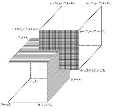
Figure 8.1: The Primal and Dual Grids Taken From [43]

primal		dual
nodes	$\left(i\,{\Delta x},j\,{\Delta y},k\,{\Delta z}\right)$	cells
	$\left(\left(i+{\frac{1}{2}}\right)\,{\Delta x},j\,{\Delta y},k\,{\Delta z}\right)$
edges	$\left(i\,{\Delta x},\left(j+{\frac{1}{2}}\right)\,{\Delta y},k\,{\Delta z}\right)$	faces
	$\left(i\,{\Delta x},j\,{\Delta y},\left(k+{\frac{1}{2}}\right)\,{\Delta z}\right)$
	$\left(i{\Delta x},\left(j+{\frac{1}{2}}\right){\Delta y},\left(k+{\frac{1}{2}}\right){\Delta z}\right)$
faces	$\left(\left(i+{\frac{1}{2}}\right){\Delta x},j{\Delta y},\left(k+{\frac{1}{2}}\right){\Delta z}\right)$	edges
	$\left(\left(i+{\frac{1}{2}}\right){\Delta x},\left(j+{\frac{1}{2}}\right){\Delta y},k{\Delta z}\right)$
cells	$\left(\left(i+{\frac{1}{2}}\right){\Delta x},\left(j+{\frac{1}{2}}\right){\Delta y},\left(k+{\frac{1}{2}}\right)\right){\Delta z}$	nodes
primal		dual

Table 8.1: Notation for the indices of the nodes and the center points of the edges, faces and cells in the primal and dual grids where $-\infty<i,j,k<\infty$.

units	primal	dual	units
$1$	$s_{i,j,k}$	$d^{\star}_{i,j,k}$	$1/d^{3}$
	$tx_{i+{\frac{1}{2}},j,k}$	$nx^{\star}_{i+{\frac{1}{2}},j,k}$
$1/d$	$ty_{i,j+{\frac{1}{2}},k}$	$ny^{\star}_{i,j+{\frac{1}{2}},k}$	$1/d^{2}$
	$tz_{i,j,k+{\frac{1}{2}}}$	$nz^{\star}_{i,j,k+{\frac{1}{2}}}$
	$nx_{i,j+{\frac{1}{2}},k+{\frac{1}{2}}}$	$tx^{\star}_{i,j+{\frac{1}{2}},k+{\frac{1}{2}}}$
$1/d^{2}$	$nz_{i+{\frac{1}{2}},j,k+{\frac{1}{2}}}$	$ty^{\star}_{i+{\frac{1}{2}},j,k+{\frac{1}{2}}}$	$1/d$
	$nz_{i+{\frac{1}{2}},j+{\frac{1}{2}},k}$	$tz^{\star}_{i+{\frac{1}{2}},j+{\frac{1}{2}},k}$
$1/d^{3}$	$d_{i+{\frac{1}{2}},j+{\frac{1}{2}},k+{\frac{1}{2}}}$	$s^{\star}_{i+{\frac{1}{2}},j+{\frac{1}{2}},k+{\frac{1}{2}}}$	$1$
units	primal	dual	units

Table 8.2: Notation for the primal and dual, scalar and vector fields where $-\infty<i,j,k<\infty$.

Mimetic discretizations use primal and dual spatial grids as shown in Figure 8.1 and the notation for the nodes, edges, faces and cells of the grid are given in Table 8.1 while the notation for scalar and vector fields are given in Table 8.2. It is important that the components of vector fields are not located at the same points in the grid. All scalar and vector fields are defined on all of space are assumed to converge to zero far from the origin. The discussion for boundary value problems is more complex and will be started in Section 10.

There two types of scalar fields and also two type of vector fields on both the primal and dual grids. On the primal grid there are scalar fields $s$ that do not have a spatial dimension, vector fields $\vec{t}$ (for tangent) that have spatial dimension $1/d$, vector fields $\vec{n}$ (for normal) that have units $1/d^{2}$, and scalar fields with spatial dimension $1/d^{3}$ (as in densities) while the dual grid has the same types of fields labeled with a superscript star as in $s^{\star}$. Note that at each point in the grid there is a value from both the primal and dual fields. These fields are different because their spatial dimensions are not the same.

Historically, this type of discretization appeared in the Yee grid for Maxwell equations [57] which will be discussed in Section 9.2.

8.2 The Discrete Double Exact Sequences

This section describes the discrete double exact sequences shown in Figure 8.2. This begins with a description of the discrete difference operators gradient, curl and divergence on the primal and dual grids. Next the star or multiplication operators that describe material properties are discretized.

$$\setcounter{MaxMatrixCols}{11}\begin{CD}{S_{\mathcal{N}}}@>{{\mathcal{G}}}>{}>{V_{\mathcal{E}}}@>{{\mathcal{R}}}>{}>{V_{\mathcal{F}}}@>{{\mathcal{D}}}>{}>{S_{\mathcal{C}}}\\ @V{a}V{}V@V{\bf A}V{}V@A{\bf B}A{}A@A{b}A{}A\\ {S_{\mathcal{C}^{\star}}}@<{{{\mathcal{D}}^{\star}}}<{}<{V_{\mathcal{F}^{\star}}}@<{{{\mathcal{R}}^{\star}}}<{}<{V_{\mathcal{E}^{\star}}}@<{{{\mathcal{G}}^{\star}}}<{}<{S_{\mathcal{N}^{\star}}}\\ \end{CD}$$

Figure 8.2: Discrete Exact Sequences

8.2.1 Difference Operators

The discrete gradient ${\mathcal{G}}$, curl or rotation ${\mathcal{R}}$ and divergence ${\mathcal{D}}$ are difference operators on a scalar or vector fields. The formulas for the dual grid are obtained by making the changes $i\rightarrow i+1/2$, $j\rightarrow j+1/2$ and $k\rightarrow k+1/2$.

The Gradient: If $s\in{S_{\mathcal{N}}}$ is a discrete scalar field, then its gradient ${\mathcal{G}}s=({\mathcal{G}}sx,{\mathcal{G}}sy,{\mathcal{G}}sz)\in{V_{\mathcal{E}}}$ is an edge vector field:

$${\mathcal{G}}sx_{i+{\frac{1}{2}},j,k}\equiv \frac{s_{i+1,j,k}-s_{i,j,k}}{\triangle x}\,;$$

$${\mathcal{G}}sy_{i,j+{\frac{1}{2}},k}\equiv \frac{s_{i,j+1,k}-s_{i,j,k}}{\triangle y}\,;$$ (8.1)

$${\mathcal{G}}sz_{i,j,k+{\frac{1}{2}}}\equiv \frac{s_{i,j,k+1}-s_{i,j,k}}{\triangle z}\,.$$

The Curl: If $\vec{t}=(tx,ty,tz)\in{V_{\mathcal{E}}}$ is a discrete edge vector field, then its curl ${\mathcal{R}}{\vec{t}}\in{V_{\mathcal{F}}}$ is a discrete face vector field:

$${\mathcal{R}}tx_{i,j+{\frac{1}{2}},k+{\frac{1}{2}}} \equiv\frac{tz_{i,j+1,k+{\frac{1}{2}}}-tz_{i,j,k+{\frac{1}{2}}}}{\triangle y}-\frac{ty_{i,j+{\frac{1}{2}},k+1}-ty_{i,j+{\frac{1}{2}},k}}{\triangle z}\,;$$

$${\mathcal{R}}ty_{i+{\frac{1}{2}},j,k+{\frac{1}{2}}} \equiv\frac{tx_{i+{\frac{1}{2}},j,k+1}-tx_{i+{\frac{1}{2}},j,k}}{\triangle z}-\frac{tz_{i+1,j,k+{\frac{1}{2}}}-tz_{i,j,k+{\frac{1}{2}}}}{\triangle x}\,;$$ (8.2)

$${\mathcal{R}}tz_{i+{\frac{1}{2}},j+{\frac{1}{2}},k} \equiv\frac{ty_{i+1,j+{\frac{1}{2}},k}-ty_{i,j+{\frac{1}{2}},k}}{\triangle x}-\frac{tx_{i+{\frac{1}{2}},j+1,k}-tx_{i+{\frac{1}{2}},j,k}}{\triangle y}\,.$$

The Divergence: If ${\vec{n}}=(nx,ny,nz)\in{V_{\mathcal{F}}}$ is a discrete face vector field, then its divergence ${\mathcal{D}}{\vec{n}}\in{S_{\mathcal{C}}}$ is a cell scalar field:

$${\mathcal{D}}{\vec{n}}_{i+{\frac{1}{2}},j+{\frac{1}{2}},k+{\frac{1}{2}}} \equiv\frac{nx_{i+1,j+{\frac{1}{2}},k+{\frac{1}{2}}}-nx_{i,j+{\frac{1}{2}},k+{\frac{1}{2}}}}{\triangle x}$$

$$+\frac{ny_{i+{\frac{1}{2}},j+1,k+{\frac{1}{2}}}-ny_{i+{\frac{1}{2}},j,k+{\frac{1}{2}}}}{\triangle y}$$ (8.3)

$$+\frac{nz_{i+{\frac{1}{2}},j+{\frac{1}{2}},k+1}-nz_{i+{\frac{1}{2}},j+{\frac{1}{2}},k}}{\triangle z}\,.$$

The Star Gradient: If $s^{\star}\in{S_{\mathcal{N}^{\star}}}$ is a discrete star scalar field then its star gradient ${{\mathcal{G}}^{\star}}\,s^{\star}\in{V_{\mathcal{E}^{\star}}}$ is a star edge vector field:

$${{\mathcal{G}}^{\star}}s^{\star}x_{i,j+{\frac{1}{2}},k+{\frac{1}{2}}} \equiv\frac{s^{\star}_{i+{\frac{1}{2}},j+{\frac{1}{2}},k+{\frac{1}{2}}}-s^{\star}_{i-{\frac{1}{2}},j+{\frac{1}{2}},k+{\frac{1}{2}}}}{\Delta x};$$

$${{\mathcal{G}}^{\star}}s^{\star}y_{i+{\frac{1}{2}},j,k+{\frac{1}{2}}} \equiv\frac{s^{\star}_{i+{\frac{1}{2}},j+{\frac{1}{2}},k+{\frac{1}{2}}}-s^{\star}_{i+{\frac{1}{2}},j-{\frac{1}{2}},k+{\frac{1}{2}}}}{\Delta x};$$ (8.4)

$${{\mathcal{G}}^{\star}}s^{\star}z_{i+{\frac{1}{2}},j+{\frac{1}{2}},k} \equiv\frac{s^{\star}_{i+{\frac{1}{2}},j+{\frac{1}{2}},k+{\frac{1}{2}}}-s^{\star}_{i+{\frac{1}{2}},j+{\frac{1}{2}},k-{\frac{1}{2}}}}{\Delta x};$$

The Star Curl: If $\vec{t}^{\star}=(tx^{\star},ty^{\star},tz^{\star})\in{S_{\mathcal{C}^{\star}}}$ is a discrete star edge vector field then its curl ${{\mathcal{R}}^{\star}}\,\vec{t}^{\star}\in{V_{\mathcal{F}^{\star}}}$ is a discrete star face vector field:

$${{\mathcal{R}}^{\star}}t^{\star}x_{i+{\frac{1}{2}},j,k} \equiv\frac{tz^{\star}_{i+{\frac{1}{2}},j+{\frac{1}{2}},k}-tz^{\star}_{i+{\frac{1}{2}},j-{\frac{1}{2}},k}}{\triangle y}-\frac{ty^{\star}_{i+{\frac{1}{2}},j,k+{\frac{1}{2}}}-ty^{\star}_{i+{\frac{1}{2}},j,k-{\frac{1}{2}}}}{\triangle z}\,;$$

$${{\mathcal{R}}^{\star}}t^{\star}y_{i,j+{\frac{1}{2}},k} \equiv\frac{tx^{\star}_{i,j+{\frac{1}{2}},k+{\frac{1}{2}}}-tz^{\star}_{i,j+{\frac{1}{2}},k-{\frac{1}{2}}}}{\triangle z}-\frac{tz^{\star}_{i+{\frac{1}{2}},j+{\frac{1}{2}},k}-tz^{\star}_{i-{\frac{1}{2}},j+{\frac{1}{2}},k}}{\triangle x}\,;$$ (8.5)

$${{\mathcal{R}}^{\star}}t^{\star}z_{i,j,k+{\frac{1}{2}}} \equiv\frac{ty^{\star}_{i+{\frac{1}{2}},j,k+{\frac{1}{2}}}-ty^{\star}_{i-{\frac{1}{2}},j,k+{\frac{1}{2}}}}{\triangle x}-\frac{tx^{\star}_{i,j+{\frac{1}{2}},k+{\frac{1}{2}}}-tx^{\star}_{i,j-{\frac{1}{2}},k+{\frac{1}{2}}}}{\triangle y}\,.$$

The Star Divergence: If $\vec{n}^{\star}=(nx^{\star},ny^{\star},nz^{\star})\in{V_{\mathcal{F}^{\star}}}$ is a discrete star face vector field then it divergence ${{\mathcal{D}}^{\star}}\vec{n}^{\star}\in{S_{\mathcal{C}^{\star}}}$ is a discrete star cell field. In terms of components

$${{\mathcal{D}}^{\star}}{\vec{n}^{\star}}_{i,j,k} \equiv\frac{nx^{\star}_{i+{\frac{1}{2}},j,k}-n^{\star}x_{i-{\frac{1}{2}},j,k}}{\triangle x}$$

$$+\frac{ny^{\star}_{i,j+{\frac{1}{2}},k}-ny^{\star}_{i,j-{\frac{1}{2}},k}}{\triangle y}$$ (8.6)

$$+\frac{nz^{\star}_{i,j,k+{\frac{1}{2}}}-nz^{\star}_{i,j,k-{\frac{1}{2}}}}{\triangle z}\,.$$

The second order accuracy of the difference operators is confirmed in TestAccuracy3.m.

8.2.2 Mimetic Properties of Difference Operators

If $c$ is a constant scalar field then a direct computation [43] shows that:

$${\mathcal{G}}c\equiv 0\,,\quad{\mathcal{R}}{\mathcal{G}}\equiv 0\,,\quad{\mathcal{D}}{\mathcal{R}}\equiv 0\,,\quad{{\mathcal{G}}^{\star}}c\equiv 0\,,\quad{{\mathcal{R}}^{\star}}{{\mathcal{G}}^{\star}}\equiv 0\,,\quad{{\mathcal{D}}^{\star}}{{\mathcal{R}}^{\star}}\equiv 0\,.$$ (8.7)

These relationships are confirmed in TestZero3.m. These properties are summarized by saying that the discretization is exact or that the sequences in Figure 8.2 are exact, see [43] for a precise definition of exact and a proof that the diagram is exact.

8.2.3 Discrete Star or Multiplication Operators

The star operators are multiplication operators that model the material properties and are given by two scalar functions $a=a(x,y,z)$ and $b=b(x,y,z)$ and two $3\times 3$ matrix functions ${\bf A}={\bf A}(x,y,z)$ and ${\bf B}={\bf B}(x,y,z)$ that are symmetric and positive. The spatial dimensions of $a$ and $b$ must be $1/s^{3}$ while for ${\bf A}$ and ${\bf B}$ must be $1/d$.

If $a_{i,j,k}=a(i\,{\Delta x},j\,{\Delta y},k\,{\Delta z})$ and if $s\in{S_{\mathcal{N}}}$ and $d^{\star}=a\,s\in{S_{\mathcal{C}^{\star}}}$ then

$$d^{\star}_{i,j,k}=a_{i,j,k}\,s_{i,j,k}\,.$$

If $b_{i,j,k}=b(i\,{\Delta x},j\,{\Delta y},k\,{\Delta z})$ and if $s^{\star}\in{S_{\mathcal{N}^{\star}}}$ and $d=b\,s^{\star}\in{S_{\mathcal{C}^{\star}}}$ then

$$d_{i,j,k}=b_{i,j,k}\,s^{\star}_{i,j,k}\,.$$

The assumption that $a$ and $b$ are not zero implies that these star operators are invertible.

Let

$${\bf A}=\left[\begin{matrix}Axx&Axy&Axy\\ Ayx&Ayy&Ayz\\ Azx&Azy&Azz\end{matrix}\right]\,,$$ (8.8)

where ${\bf A}$ is symmetric, positive definite, and the entries in ${\bf A}$ are functions of $(x,y,z)$. The discretized ${\bf A}$ will not be symmetric but will be nearly symmetric.

For ${\vec{t}}\in{V_{\mathcal{E}}}$, computing ${\vec{n}}^{\star}={\bf A}\vec{t}\in{S_{\mathcal{N}^{\star}}}$ requires averaging of the off diagonal terms in ${\bf A}$ to maintain second order accuracy. First set

$$nx^{\star}_{i+{\frac{1}{2}},j,k}= Axx_{i+{\frac{1}{2}},j,k}\,tx_{i+{\frac{1}{2}},j,k}+Axy_{i+{\frac{1}{2}},j,k}\,\overline{ty}_{i+{\frac{1}{2}},j,k}+Axz_{i+{\frac{1}{2}},j,k}\,\overline{tz}_{i+{\frac{1}{2}},j,k}$$

$$ny^{\star}_{i,j+{\frac{1}{2}},k}= Ayx_{i,j+{\frac{1}{2}},k}\,\overline{tx}_{i,j+{\frac{1}{2}},k}+Ayy_{i,j+{\frac{1}{2}},k}\,ty_{i,j+{\frac{1}{2}},k}+Ayz_{i,j+{\frac{1}{2}},k}\,\overline{tz}_{i,j+{\frac{1}{2}},k}$$ (8.9)

$$nz^{\star}_{i,j,k+{\frac{1}{2}}}= Ayx_{i,j,k+{\frac{1}{2}}}\,\overline{tx}_{i,j,k+{\frac{1}{2}}}+Ayy_{i,j,k+{\frac{1}{2}}}\,\overline{ty}_{i,j,k+{\frac{1}{2}}}+Ayz_{i,j,k+{\frac{1}{2}}}\,tz_{i,j,k+{\frac{1}{2}}}\,.$$

The average values are given by

$$\overline{ty}_{i+{\frac{1}{2}},j,k} =\frac{ty_{i,j-{\frac{1}{2}},k}+ty_{i,j+{\frac{1}{2}},k}+ty_{i+1,j-{\frac{1}{2}},k}+ty_{i+1,j+{\frac{1}{2}},k}}{4}\,,$$

$$\overline{tz}_{i+{\frac{1}{2}},j,k} =\frac{tz_{i,j,k-{\frac{1}{2}}}+tz_{i,j,k+{\frac{1}{2}}}+tz_{i+1,j,k-{\frac{1}{2}}}+tz_{i+1,j,k+{\frac{1}{2}}}}{4}\,,$$

$$\overline{tx}_{i,j+{\frac{1}{2}},k} =\frac{tx_{i,j-{\frac{1}{2}},k}+tx_{i,j+{\frac{1}{2}},k}+tx_{i+1,j-{\frac{1}{2}},k}+tx_{i+1,j+{\frac{1}{2}},k}}{4}\,,$$

$$\overline{tz}_{i,j+{\frac{1}{2}},k} =\frac{tz_{i,j,k-{\frac{1}{2}}}+tz_{i,j,k+{\frac{1}{2}}}+tz_{i,j+1,k-{\frac{1}{2}}}+tz_{i,j+1,k+{\frac{1}{2}}}}{4}\,,$$

$$\overline{tx}_{i,j,k+{\frac{1}{2}}} =\frac{tx_{i-{\frac{1}{2}},j,k}+tx_{i+{\frac{1}{2}},j,k}+tx_{i-{\frac{1}{2}},j,k+1}+tx_{i+{\frac{1}{2}},j,k+1}}{4}\,,$$

$$\overline{ty}_{i,j,k+{\frac{1}{2}}} =\frac{ty_{i,j-{\frac{1}{2}},k}+ty_{i,j+{\frac{1}{2}},k}+ty_{i,j-{\frac{1}{2}},k+1}+ty_{i,j+{\frac{1}{2}},k+1}}{4}\,.$$

Note that if ${\bf A}$ is diagonal then multiplication by ${\bf A}$ is simply multiplication by the diagonal entries of ${\bf A}$ and no averaging is required. There are similar formulas for multiplication by ${\bf B}$, ${\bf A}^{-1}$ and ${\bf B}^{-1}$. Many of the second order operators in Table 6.2 have a multiplication by the inverse of ${\bf A}$ and/or ${\bf B}$. It is assumed that the matrix operators are given by formulas, and formulas for the inverse operators can be found and so that the formulas above can be used to multiply by the inverse matrices.

8.3 Discrete Inner Products

To study conserved quantities an inner product is needed for each of the eight linear spaces in the dual exact sequences Figure (8.2). The inner products will be defined in terms of four bilinear forms as in 6.2. As in the continuum, an important property of the inner products is that they need to be symmetric, positive definite and importantly dimensionless.

Four bilinear forms will be needed. Set $\Delta V=\Delta x\,\Delta y\,\Delta z$.

If $s\in{S_{\mathcal{N}}}$ and $d^{\star}\in{S_{\mathcal{C}^{\star}}}$ then

$$\langle\langle s,d\rangle\rangle=\sum s_{i,j,k}\,d^{\star}_{i,j,k}\,\Delta V\,.$$

If $\vec{t}\in{V_{\mathcal{E}}}$ and $\vec{n}^{\star}\in{V_{\mathcal{F}^{\star}}}$ then

$$\langle\langle\vec{t},\vec{n}^{\star}\rangle\rangle=\left(\sum tx_{i+{\frac{1}{2}},j,k}\,nx^{\star}_{i+{\frac{1}{2}},j,k}+\sum ty_{i,j+{\frac{1}{2}},k}\,ny^{\star}_{i,j+{\frac{1}{2}},k}+\sum tz_{i,j,k+{\frac{1}{2}}}\,nz^{\star}_{i,j,k+{\frac{1}{2}}}\right)\Delta V\,.$$

If $\vec{n}\in{V_{\mathcal{E}}}$ and $\vec{t}^{\star}\in{V_{\mathcal{F}^{\star}}}$ then

$$\langle\langle\vec{n},\vec{t}^{\star}\rangle\rangle=\left(\sum nx_{i,j+{\frac{1}{2}},k+{\frac{1}{2}}}\,tx^{\star}_{i,j+{\frac{1}{2}},k+{\frac{1}{2}}}+\sum ny_{i+{\frac{1}{2}},j,k+{\frac{1}{2}}}\,ty^{\star}_{i+{\frac{1}{2}},j,k+{\frac{1}{2}}}+\sum nz_{i+{\frac{1}{2}},j+{\frac{1}{2}},k}\,tz^{\star}_{i+{\frac{1}{2}},j+{\frac{1}{2}},k}\right)\Delta V\,.$$

If $g\in{S_{\mathcal{C}}}$ and $f^{\star}\in{S_{\mathcal{N}^{\star}}}$ then

$$\langle\langle g,f^{\star}\rangle\rangle=\sum g_{i+{\frac{1}{2}},j+{\frac{1}{2}},k+{\frac{1}{2}}}\,f^{\star}_{i+{\frac{1}{2}},j+{\frac{1}{2}},k+{\frac{1}{2}}}\Delta V\,.$$

The eight inner products are given by are given by the bilinear forms.

If $s1,s2\in{S_{\mathcal{N}}}$ then $\langle s1,s2\rangle_{\mathcal{N}}=\langle\langle a\,s1,s2\rangle\rangle$.

If $s1^{\star},s2^{\star}\in{S_{\mathcal{N}^{\star}}}$ then

$$\langle s1^{\star},s2^{\star}\rangle_{{\mathcal{N}}^{\star}}=\sum_{i,j,k}b_{i+{\frac{1}{2}},j+{\frac{1}{2}},k+{\frac{1}{2}}}\,s1^{\star}_{i+{\frac{1}{2}},j+{\frac{1}{2}},k+{\frac{1}{2}}}\,s2^{\star}_{i+{\frac{1}{2}},j+{\frac{1}{2}},k+{\frac{1}{2}}}\triangle x\triangle y\triangle z\,.$$

If $\vec{t1},\vec{t2}\in{V_{\mathcal{E}}}$ then

$$\langle\vec{t1},\vec{t2}\rangle_{\mathcal{E}}=\sum_{i,j,k}( ({\bf A}\,\vec{t1})_{i+{\frac{1}{2}},j,k}\,\vec{t2}_{i+{\frac{1}{2}},j,k}+$$

$$({\bf A}\,\vec{t1})_{i,j+{\frac{1}{2}},k}\,\vec{t2}_{i,j+{\frac{1}{2}},k}+$$

$$({\bf A}\,\vec{t1})_{i,j,k+{\frac{1}{2}}}\,\vec{t2}_{i,j,k+{\frac{1}{2}}})\triangle x\triangle y\triangle z$$

If $\vec{t1}^{\star},\vec{t2}^{\star}\in{V_{\mathcal{E}^{\star}}}$ then

$$\langle\vec{t1}^{\star},\vec{t2}^{\star}\rangle_{{\mathcal{E}}^{\star}}=\sum_{i,j,k}( ({\bf B}\,\vec{t1}^{\star})_{i,j+{\frac{1}{2}},k+{\frac{1}{2}}}\,\vec{t2}^{\star}_{i,j+{\frac{1}{2}},k+{\frac{1}{2}}}+$$

$$({\bf B}\,\vec{t1}^{\star})_{i,+{\frac{1}{2}}j,k+{\frac{1}{2}}}\,\vec{t2}^{\star}_{i+{\frac{1}{2}},j,k+{\frac{1}{2}}}+$$

$$({\bf B}\,\vec{t1}^{\star})_{i+{\frac{1}{2}},j+{\frac{1}{2}},k}\,\vec{t2}^{\star}_{i+{\frac{1}{2}},j+{\frac{1}{2}},k})\triangle x\triangle y\triangle z$$

If $\vec{n1},\vec{n2}\in{V_{\mathcal{F}}}$ then

$$\langle\vec{n1},\vec{n2}\rangle_{\mathcal{F}}=\sum_{i,j,k}( ({\bf B}^{-1}\,n1)_{i,j+{\frac{1}{2}},k+{\frac{1}{2}}}\,n2{i,j+{\frac{1}{2}},k+{\frac{1}{2}}}+$$

$$({\bf B}^{-1}\,n1)_{i,+{\frac{1}{2}}j,k+{\frac{1}{2}}}\,n2{i+{\frac{1}{2}},j,k+{\frac{1}{2}}}+$$

$$({\bf B}^{-1}\,n1)_{i+{\frac{1}{2}},j+{\frac{1}{2}},k}\,n2{i+{\frac{1}{2}},j+{\frac{1}{2}},k})\triangle x\triangle y\triangle z$$

If $\vec{n1}^{\star},\vec{n2}^{\star}\in{V_{\mathcal{F}^{\star}}}$ then

$$\langle\vec{n1}^{\star},\vec{n2}^{\star}\rangle_{{\mathcal{F}}^{\star}}=\sum_{i,j,k}( ({\bf A}^{-1}\,n1)^{\star}_{i+{\frac{1}{2}},j,k}\,n2^{\star}_{i+{\frac{1}{2}},j,k}+$$

$$({\bf A}^{-1}\,n1)^{\star}_{i,j+{\frac{1}{2}},k}\,n2^{\star}_{i,j+{\frac{1}{2}},k}+$$

$$({\bf A}^{-1}\,n1)^{\star}_{i,j,k+{\frac{1}{2}}}\,n2^{\star}_{i,j,k+{\frac{1}{2}}})\triangle x\triangle y\triangle z$$

If $d1,d2\in{S_{\mathcal{C}}}$ then

$$\langle d1,d2\rangle_{\mathcal{N}}=\sum_{i,j,k}b^{-1}_{i+{\frac{1}{2}},j+{\frac{1}{2}},k+{\frac{1}{2}}}\,d1_{i+{\frac{1}{2}},j+{\frac{1}{2}},k+{\frac{1}{2}}}\,d2_{i+{\frac{1}{2}},j+{\frac{1}{2}},k+{\frac{1}{2}}}\triangle x\triangle y\triangle z\,.$$

If $d1^{\star},d2^{\star}\in{S_{\mathcal{C}^{\star}}}$ then

$$\langle d1^{\star},d2^{\star}\rangle_{{\mathcal{C}}^{\star}}=\sum_{i,j,k}a^{-1}_{i,j,k}\,d1^{\star}_{i,j,k}\,d2^{\star}_{i,j,k}\triangle x\triangle y\triangle z\,.$$

8.4 Adjoint Operators

The derivation of the adjoints of the discrete operators in the discrete exact sequences shown in Figure 8.2 are similar to the derivation for the continuum the adjoint operators defined in Section 6.5. Again note that the discrete operators are not mapping of a space into itself. The adjoints can easily be derived by diagram chasing using 8.2.

$${\mathcal{G}}^{*} =-a^{-1}\,{{\mathcal{D}}^{\star}}\,{\bf A} {{\mathcal{G}}^{\star}}^{*} =-b^{-1}\,{\mathcal{D}}\,{\bf B}\,,$$

$${\mathcal{R}}^{*} =+{\bf A}^{-1}\,{{\mathcal{R}}^{\star}}\,{\bf B}^{-1} {{\mathcal{R}}^{\star}}^{*} =+{\bf B}^{-1}\,{\mathcal{R}}\,{\bf A}^{-1}\,,$$

$${\mathcal{D}}^{*} =-{\bf B}{{\mathcal{G}}^{\star}}b^{-1} {{\mathcal{D}}^{\star}}^{*} =-{\bf A}{\mathcal{G}}a^{-1}\,,$$

$${\bf A}^{*} ={\bf A}^{-1} {\bf B}^{*} ={\bf B}^{-1}\,,$$ (8.10)

$$a^{*} =a^{-1} b^{*} =b^{-1}\,.$$

The proofs of the adjoint formulas rely of summation by parts which is illustrate by computing

$$\sum_{i,j,k}\left(s_{i+1,j,k}-s_{i,j,k}\right)\,n^{\star}_{i+{\frac{1}{2}},j,k} =\sum_{i,j,k}s_{i+1,j,k}\,n^{\star}_{i+{\frac{1}{2}},j,k}-\sum_{i,j,k}s_{i,j,k}\,n^{\star}_{i+{\frac{1}{2}},j,k}$$

$$=\sum_{i,j,k}s_{i,j,k}\,n^{\star}_{i-{\frac{1}{2}},j,k}-\sum_{i,j,k}s_{i,j,k}\,n^{\star}_{i+{\frac{1}{2}},j,k}$$

$$=\sum_{i,j,k}s_{i,j,k}\,\left(n^{\star}_{i-{\frac{1}{2}},j,k}-n^{\star}_{i+{\frac{1}{2}},j,k}\right)$$

$$=-\sum_{i,j,k}s_{i,j,k}\,\left(n^{\star}_{i+{\frac{1}{2}},j,k}-n^{\star}_{i-{\frac{1}{2}},j,k}\right)$$

The remaining proofs are straight forward. Others have used summation by parts to obtain mimetic like discretizations [55, 15, 34].

When working with systems of first order wave equation and second order wave equation additional adjoints will be needed:

$$({\bf A}{\mathcal{G}})^{*}={\mathcal{G}}^{*}{\bf A}=a^{-1}{\mathcal{D}}^{*}{\bf A}{\bf A}^{-}1=a^{-1}{\mathcal{D}}^{*}\,.$$

8.5 Positive and Negative Discrete Operators

If $s\in\in{S_{\mathcal{N}}}$ and $\vec{n}^{\star}\in{V_{\mathcal{F}^{\star}}}$ then

$$\langle{\bf A}\,{\mathcal{G}}\,s,\vec{n}^{\star}\rangle_{{\mathcal{F}}^{\star}}=-\langle s,\frac{1}{a}\,{{\mathcal{D}}^{\star}}\,\vec{n}^{\star}\rangle_{\mathcal{N}}$$ (8.11)

If $\vec{t}\in{V_{\mathcal{E}}}$ and $\vec{t}^{\star}\in{V_{\mathcal{E}^{\star}}}$ then

$$\langle{\bf B}^{-1}\,{\mathcal{R}}\vec{t},\vec{t}^{\star}\rangle_{{\mathcal{E}}^{\star}}=-\langle\vec{t}\,,{\bf A}^{-1}{{\mathcal{R}}^{\star}}\vec{t}^{\star}\rangle_{\mathcal{E}}$$ (8.12)

If $\vec{n}\in{V_{\mathcal{F}}}$ and $\vec{t}^{\star}\in{S_{\mathcal{N}^{\star}}}$ then

$$\langle b^{-1}\,{\mathcal{D}}\vec{n},s^{\star}\rangle_{{\mathcal{N}}^{\star}}=-\langle\vec{n}\,,{\bf B}{{\mathcal{G}}^{\star}}\vec{s}^{\star}\rangle_{\mathcal{F}}$$ (8.13)

For an example, consider (8.11):

$$\langle{\bf A}\,{\mathcal{G}}\,s,\vec{n}^{\star}\rangle_{{\mathcal{F}}^{\star}}=$$

$$\sum_{i,j,k}\left(\frac{s_{i+1,j,k}-s_{i,j,k}}{\triangle x}\,n^{\star}_{i+{\frac{1}{2}},j,k}+\frac{s_{i,j+1,k}-s_{i,j,k}}{\triangle y}\,n^{\star}_{i,j+{\frac{1}{2}},k}+\frac{s_{i,j,k+1}-s_{i,j,k}}{\triangle z}\,n^{\star}_{i,j,k+{\frac{1}{2}}}\right)\triangle x\triangle y\triangle z$$

$$\langle s,\frac{1}{a}\,{{\mathcal{D}}^{\star}}\,\vec{n}^{\star}\rangle_{\mathcal{N}}=$$

$$\sum_{i,j,k}s_{i,j,k}\,\left(\frac{n^{\star}_{i+{\frac{1}{2}},j,k}-n^{\star}_{i-{\frac{1}{2}},j,k}}{\triangle x}+\frac{n^{\star}_{i,j+{\frac{1}{2}},k}-n^{\star}_{i,j-{\frac{1}{2}},k}}{\triangle y}+\frac{n^{\star}_{i,j,k+{\frac{1}{2}}}-n^{\star}_{i,j,k-{\frac{1}{2}}}}{\triangle z}\right)\triangle x\triangle y\triangle z\,.$$

Three summation by parts will prove (8.11). The remaining formulas (8.12) and (8.13) can be proved in the same way.

9 Discretizing Wave Equations in 3D

The previous results will be used to discretize the scalar wave equation and Maxwell’s wave equation in three dimensions. Here the simulation region is all space, boundary conditions for bound domain will be discussed later.

9.1 The Scalar Wave Equation

The second order scalar wave equation (7.1) can be written as as first order system as in (7.8). But here the notation will be changed to match that in Section 8:

$$\frac{\partial s}{\partial t}=a^{-1}{\vec{\nabla}\boldsymbol{\cdot}}\,\vec{v}\,,\quad\frac{\partial\vec{v}}{\partial t}={\bf A}{\vec{\nabla}}s\,,$$

with $s\in H_{P}$ and $\vec{v}\in H_{S}$. This system will be discretized using the operators described in Section 8 so now let $s\in{S_{\mathcal{N}}}$ and $v\in{V_{\mathcal{F}^{\star}}}$ and then the leapfrog discretization is

$$\frac{s^{n+1}-s^{n}}{\triangle t}=a^{-1}\,{{\mathcal{D}}^{\star}}v^{n+{\frac{1}{2}}}\,,\quad\frac{v^{n+{\frac{1}{2}}}-v^{n-{\frac{1}{2}}}}{\triangle t}={\bf A}{\mathcal{G}}s^{n}\,.$$ (9.1)

If $s^{0}$ and $v^{{\frac{1}{2}}}$ are given then the leapfrog scheme for $n\geq 0$ is

$$s^{n+1}=s^{n}+\triangle t\,a^{-1}\,{{\mathcal{D}}^{\star}}v^{n+{\frac{1}{2}}}\,,\quad v^{n+{\frac{3}{2}}}=v^{n+{\frac{1}{2}}}+\triangle t\,{\bf A}{\mathcal{G}}s^{n+1}\,.$$

This gives a discretization of a second order scalar wave equation (7.1) as

$$\frac{s^{n+1}-2\,s^{n}+s^{n-1}}{\triangle t^{2}}=a^{-1}\,{{\mathcal{D}}^{\star}}{\bf A}{\mathcal{G}}s^{n}\,,$$ (9.2)

and as discussed in Section 7 on continuum wave equations.

This is also a discretization of the vector wave equation

$$\frac{v^{n+{\frac{3}{2}}}-2\,v^{n+{\frac{1}{2}}}+v^{n-{\frac{1}{2}}}}{\triangle t^{2}}={\bf A}{\mathcal{G}}a^{-1}\,{{\mathcal{D}}^{\star}}v^{n+{\frac{1}{2}}}\,.$$ (9.3)

The results in Section 3 give two conserved quantities for the discretization. To see this using (3.5) and (3.6) set $A$ to $a^{-1}\,{{\mathcal{D}}^{\star}}$, $A^{*}$ to $-{\bf A}{\mathcal{G}}$, $g^{n+{\frac{1}{2}}}$ to $v^{n+{\frac{1}{2}}}$ and $f^{n}$ to $s^{n}$ to get the conserved conserved quantities

$$C^{n}=\left|\left|s^{n}\right|\right|_{\mathcal{N}}^{2}+\left|\left|\frac{v^{n+1/2}+v^{n-1/2}}{2}\right|\right|_{{\mathcal{F}}^{\star}}^{2}-\frac{\Delta t^{2}}{4}\left|\left|{\bf A}{\mathcal{G}}\,s^{n}\right|\right|_{{\mathcal{F}}^{\star}}^{2}\,,$$ (9.4)

$$C^{n+1/2}=\left|\left|v^{n+1/2}\right|\right|_{{\mathcal{F}}^{\star}}^{2}+\left|\left|\frac{s^{n+1}+s^{n}}{2}\right|\right|_{\mathcal{N}}^{2}-\frac{\Delta t^{2}}{4}\left|\left|a^{-1}\,{{\mathcal{D}}^{\star}}\,v^{n+1/2}\right|\right|_{\mathcal{N}}^{2}\,.$$ (9.5)

These formulas agree with those derived in detail in Appendix B.

The programs ScalarWave.m and ScalarWaveStar.m were used to show that the energies $C_{n}$ and $C_{n+{\frac{1}{2}}}$ are constant to less than 1 part in $10^{15}$ for the discretization described above and the one that changes ${\mathcal{G}}$ to ${{\mathcal{G}}^{\star}}$ and ${{\mathcal{D}}^{\star}}$ to ${\mathcal{D}}$.

9.2 Maxwell’s Equations

Assume that ${\vec{E}}\in{V_{\mathcal{E}}}$ and $\vec{H}\in{V_{\mathcal{E}^{\star}}}$ so that, using the notation in the previous sections, the Maxwell system 5.9 will be discretized as

$$\frac{{\vec{E}}^{n+1}-{\vec{E}}^{n}}{\triangle t}=\epsilon^{-1}\,{{\mathcal{R}}^{\star}}\vec{H}^{n+{\frac{1}{2}}}\,,\quad\frac{\vec{H}^{n+{\frac{1}{2}}}-\vec{H}^{n-{\frac{1}{2}}}}{\triangle t}=-\mu^{-1}\,{\mathcal{R}}{\vec{E}}^{n}\,.$$

where in Exact Sequence diagram (8.2) $A=\epsilon$ and $B=\mu$. Here $\epsilon$ and $\mu$ can be symmetric positive definite matrices. If $\vec{E}=(Ex,Ey,Ez)$ and $\vec{H}=(Hx,Hy,Hz)$ then Table 8.1 shows that $Ex$ and $Hx$ are indexed as

$$Ex^{n}_{i+{\frac{1}{2}},j,k}\,,\quad Hx^{n+{\frac{1}{2}}}_{i,j+{\frac{1}{2}},k+{\frac{1}{2}}}$$

just as in Yee’s paper [57]. If $\vec{E}^{0}$ and $\vec{H}^{\frac{1}{2}}$ are given then the leapfrog scheme for $n\geq 0$ is

$${\vec{E}}^{n+1}={\vec{E}}^{n}+\triangle t\,\epsilon^{-1}\,{{\mathcal{R}}^{\star}}\vec{H}^{n+{\frac{1}{2}}}\,,\quad\vec{H}^{n+3/2}=\vec{H}^{n+{\frac{1}{2}}}-\triangle t\,\mu^{-1}\,{\mathcal{R}}{\vec{E}}^{n+1}\,.$$

Using a similar argument, it is easy to see that

$$C_{n+1/2}=\left|\left|\frac{\vec{E}^{n+1}+\vec{E}^{n}}{2}\right|\right|_{\mathcal{E}}^{2}+\left|\left|\vec{H}^{n+1/2}\right|\right|_{{\mathcal{E}}^{\star}}^{2}-\frac{\Delta t^{2}}{4}\left|\left|\epsilon^{-1}\,{{\mathcal{R}}^{\star}}\,\vec{H}^{n+1/2}\right|\right|_{\mathcal{E}}^{2}$$

is a conserved quantity and that

$$C_{n+1/2}\geq\left|\left|\frac{\vec{E}^{n+1}+\vec{E}^{n}}{2}\right|\right|_{\mathcal{E}}^{2}+\left(1-\frac{\Delta t^{2}}{4}\left|\left|\epsilon^{-1}\,{{\mathcal{R}}^{\star}}\right|\right|^{2}\right)\left|\left|\vec{H}^{n+1/2}\right|\right|_{{\mathcal{E}}^{\star}}^{2}\,.$$

So $C_{n+1/2}\geq 0$ for $\Delta t$ sufficiently small provided $\left|\left|\epsilon^{-1}\,{{\mathcal{R}}^{\star}}\right|\right|$ is finite.

Also

$$C_{n}=\left|\left|\vec{E}^{n}\right|\right|_{\mathcal{E}}^{2}-\frac{\Delta t^{2}}{4}\left|\left|\mu^{-1}{\mathcal{R}}\,\vec{E}^{n}\right|\right|_{{\mathcal{F}}^{\star}}^{2}+\left|\left|\frac{\vec{H}^{n+1/2}+\vec{H}^{n-1/2}}{2}\right|\right|_{{\mathcal{F}}^{\star}}^{2}\,.$$

is a conserved quantity and

$$\left|\left|C_{n}\right|\right|\geq\left(1-\frac{\Delta t^{2}}{4}\left|\left|\mu^{-1}{\mathcal{R}}\right|\right|^{2}\right)\left|\left|\vec{E}^{n}\right|\right|_{\mathcal{E}}^{2}+\left|\left|\frac{\vec{H}^{n+1/2}+\vec{H}^{n-1/2}}{2}\right|\right|_{{\mathcal{F}}^{\star}}^{2}\,.$$

So $\left|\left|C_{n}\right|\right|$ is positive for sufficiently small $\Delta t$ if $\left|\left|\mu^{-1}{\mathcal{R}}\,\vec{E}^{n}\right|\right|$ is finite. Also, these formulas agree with those derived in detail in Appendix B.

The codes Maxwell.m and MaxwellStar.m confirm that our algorithms conserve $C_{n+1/2}$ and $C_{n}$ to two parts in $10^{16}$. Additionally, the divergence of the curl of the electric and magnetic fields are constant to one part in $10^{14}$ when there are no sources.

10 Implementation in 2D

The goal is to illustrate how scalar and vector functions are discretized in 2D and then show how the gradient and divergence are discretized. This will provide some intuition on how to discretize functions and differential operators in 3D. For 3D the primal and dual grids are shown in Figure 8.1 and described in Table 8.1. In some ways the 2D discretization is more complicated than the 3D because in 3D cells have edges and faces while in 2D the edge of a cell can correspond to either an edge or a face in 3D.

The implementation of mimetic finite difference discretizations in a bounded region can be annoying due to the two staggered grids and indices that contain a half. Additionally, the components of vector fields are discretized at different points. There are also problems at the boundary that the star operators will be used fix. Initially the star operators will be trivial, except at the boundary. The simulation region will be the unit square.

For 3D a detailed description of the mimetic discretization is given in Section 8. In particular the left most box in Figure 8.2 will be used for the 2D discretization.

To facilitate programming, all indices are integers greater than zero, for example $i\geq 1$ and $j\geq 1$.

10.1 The 2D primal and dual grids

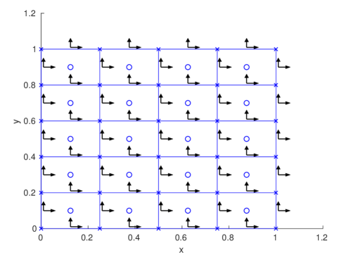
Figure 10.1: 2D primal grid tangent and normal vector fields, $Nx=4$, $Ny=5$

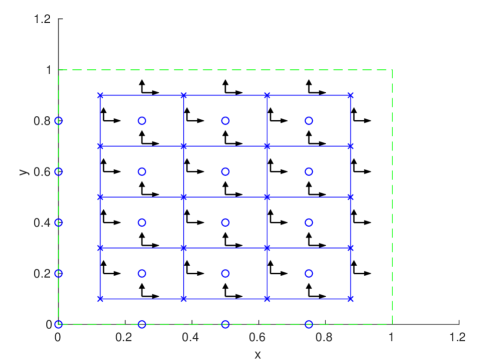
Figure 10.2: 2D dual grid tangent and normal vector fields, $Nx=4$, $Ny=5$

Let $Nx,Ny$ be positive integers and then set $dx=1/Nx$, $dy=1/Ny$. The primal grid nodes (cell corners) are given by

$$(xp(i,j),yp(i,j)) =((i-1)\,dx,(j-1)\,dy)\,,\quad 1\leq i\leq Nx+1\,,1\leq j\leq Ny+1\,,$$

and the dual grid nodes are given by

$$(xd(i,j),yd(i,j)) =((i-1/2)\,dx,(j-1/2)\,dy)\,,\quad 1\leq i\leq Nx\,,1\leq j\leq Ny\,.$$

Note that in the primal grid $Nx$ is the number of cells in $x$ direction and $Ny$ is the number of cells in the $y$ direction. For $Nx=4$ and $Ny=5$ the positions of scalar and vector function on the primal and dual grids are illustrated in Figures 10.1 and 10.2, see FigurePrimalDual2.m. Compare these to Figure 8.1 for a 3D grid.

Important points are that a primal grid cell center is given by a dual grid node and the dual grid centers are given by given by the interior primal grid nodes. Additionally the location of dual grid tangent vectors are the same as the location of the primal grid interior normal vectors and the position of the dual grid normal vectors are the same as the position of the interior grid tangent vectors. On the boundary of the primal grid the positions of points and vectors do not correspond to anything in the dual grid. As will be seen this is important for representing boundary conditions for partial differential equations.

10.2 Discretizing continuum functions on the 2D grids

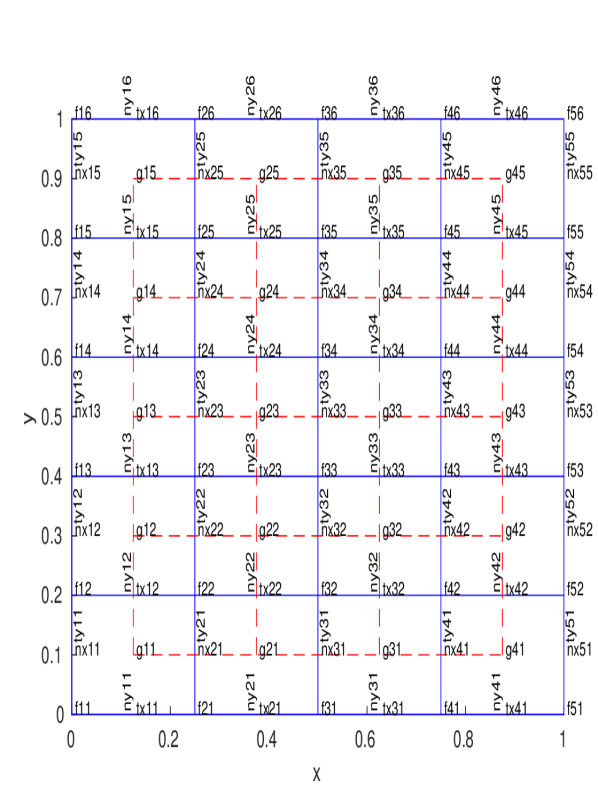
Figure 10.3: Scalar and vector fields on the primal grid.

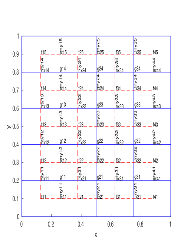
Figure 10.4: Scalar and vector fields on the dual grid,

Scalar functions will be discretized at either the nodes (corners) or cell centers of the primal and dual grids while vector fields will be discretized at the centers of the of the edges of the cells as illustrated in Figures 10.1 and 10.2 for grids in a region that is a unit square (see FigureDetailsPrimalDual2.m). There are a total of eight types of discretized functions. In the text, function names on the primal grid have a $p$ appended as in $fp$ while functions on the dual grid have a $d$ appended as in $fd$. In the figures which grid the functions are on is clear.

For the primal grid there are four cases. A scalar function $f(x,y)$ with spatial weight $1$ is discretized at primal cell nodes:

$$fp(i,j)=f(xp(i),yp(j))\,,\quad i\leq Nx+1\,,\quad j\leq Ny+1\,.$$ (10.1)

A scalar function $g(x,y)$ with spatial weights $1/d^{3}$ is discretized at primal grid cell centers:

$$gp(i,j)=g(xd(i),yd(j))\,,\quad i\leq Nx\,,\quad j\leq Ny\,.$$ (10.2)

A vector function $(tx(x,y),ty(x,y)$ with spatial weight $1/d$ (tangent on primal grid) is discretized at cell edge centers:

$$txp(i,j)= tx(xd(i),yp(j))\,,\quad i\leq Nx\,,\quad j\leq Ny+1\,;$$ (10.3)

$$typ(i,j)= ty(xp(i),yd(j))\,,\quad i\leq Nx+1\,,\quad j\leq Ny\,.$$ (10.4)

A vector function $(nx(x,y),ny(x,y)$ with spatial weight $1/d^{2}$ (normal on primal grid) is also discretized at cell edge centers:

$$nxp(i,j)= nx(xp(i),yd(i))\,,\quad i\leq Nx+1\,,\quad j\leq Ny\,;$$ (10.5)

$$nyp(i,j)= ny(xd(i),yp(j))\,,\quad i\leq Nx\,,\quad j\leq Ny+1\,.$$ (10.6)

For the dual grid there are also four cases. A scalar function $f(x,y)$ with spatial weight $1$ is discretized at the dual cell nodes:

$$fd(i,j)=f(xd(i),yd(j))\,,\quad i\leq Nx\,,\quad j\leq Ny\,.$$ (10.7)

A scalar function $g(x,y)$ with spatial weights $1/d^{3}$ is discretized at dual grid cell centers nodes:

$$gd(i,j)=g(xp(i+1),yp(j+1))\,,\quad i\leq Nx-1\,,\quad j\leq Ny-1\,.$$ (10.8)

A vector function $(tx(x,y),ty(x,y)$ with spatial weight $1/d$ (tangent on dual grid) is discretized at cell edge centers:

$$txd(i,j)= tx(xp(i+1),yd(j))\,,\quad i\leq Nx-1\,,\quad j\leq Ny\,;$$ (10.9)

$$tyd(i,j)= ty(xd(i),yp(j+1))\,,\quad i\leq Nx\,,\quad j\leq Ny\,.$$ (10.10)

A vector function $(nx(x,y),ny(x,y)$ with spatial weight $1/d^{2}$ (normal on the dual grid) is discretized at cell face centers:

$$nxd(i,j)= nx(xd(i),yp(j+1))\,,\quad i\leq Nx\,,\quad j\leq Ny-1\,;$$ (10.11)

$$nyd(i,j)= ny(xp(i+1),yd(j))\,,\quad i\leq Nx-1\,,\quad j\leq Ny\,.$$ (10.12)

Examples of 2D scalar and vector fields can be generated using ScalarField2p.m, ScalarField2d.m, TangentField2p.m, TangentField2d.m, NormalField2p.m, NormalField2d.m, DensityField2p.m, DensityField2d.m and tested using TestFields2pd.m

10.3 The Star Operators

For simplicity the discussion of star operators will begin for material properties that are constant. These star operators will map quantities defined on the primal grid to the dual grid while their inverses do the opposite. For constant and isotropic materials the star operators are multiplication by a constant for quantities that are defined at the same point in the grids. For scalar variables this is done by multiplication by a constant $a>0$ with spatial dimension $1/d^{3}$. For vectors a constant diagonal matrix

$${\bf A}=\left[\begin{matrix}A11&0\\ 0&A22\\ \end{matrix}\right]$$

with $A11>0$ and $A22>0$ spatial dimension $1/d$ will be used. If $A11\neq A22$ then there is a simple anisotropy. Away from the boundaries of the region, the two star operators are inverses of each other. For boundary value problems, the mismatch between the sizes of the primal and dual grids will be used to represent the boundary conditions. The star operators will be given in pairs that are essentially inverse of each other, first the mapping from the primal grid to the dual grid and then the inverse.

If $gd=\star fp$ then

$$gd(i,j)=a\,fp(i+1,j+1)\,,\quad 1\leq i\leq N_{x}-1\,,\quad 1\leq j\leq N_{y}-1\,.$$ (10.13)

If $fp=\star gd$ then

$$fp(i,j)=\frac{1}{a}\,gd(i-1,j-1)\,,\quad 2\leq i\leq N_{x}\,,\quad 2\leq j\leq N_{y}\,.$$ (10.14)

In this case $fp$ is not defined on the boundary of the primal grid.

If $fd=\star gp$ then

$$gp(i,j)=a\,fd(i,j)\,,\quad 1\leq i\leq N_{x}\,,\quad 1\leq j\leq N_{y}\,.$$ (10.15)

If $gp=\star fd$ then

$$gp(i,j)=\frac{1}{a}\,fd(i,j)\,,\quad 1\leq i\leq N_{x}\,,\quad 1\leq j\leq N_{y}\,.$$ (10.16)

If $(txd,tyd)=\star(nxp,nyp)$ then

$$txd(i,j) =\frac{1}{A11}\,nxp(i+1,j)\,,\quad 1\leq i\leq N_{x}-1\,,\quad 1\leq j\leq N_{y}\,.$$

$$tyd(i,j) =\frac{1}{A22}\,nyp(i,j+1)\,,\quad 1\leq i\leq N_{x}\,,\quad 1\leq j\leq N_{y}-1\,.$$ (10.17)

If $(nxp,nyp)=\star(txd,tyd)$ then

$$nxp(i,j) =A11\,txd(i-1,j)\,,\quad 2\leq i\leq N_{x}\,,\quad 1\leq j\leq N_{y}\,.$$

$$nyp(i,j) =A22\,tyd(i,j-1)\,,\quad 1\leq i\leq N_{x}\,,\quad 2\leq j\leq N_{y}\,.$$ (10.18)

If $(nxd,nyd)=\star(txp,typ)$ then

$$nxd(i,j) =A11\,txp(i,j+1)\,,\quad 1\leq i\leq N_{x}\,,\quad 1\leq j\leq N_{y}-1\,.$$

$$nyd(i,j) =A22\,typ(i+1,j)\,,\quad 1\leq i\leq N_{x}-1\,,\quad 1\leq j\leq N_{y}\,.$$ (10.19)

If $(txp,typ)=\star(nxd,nyd)$ then

$$txp(i,j) =\frac{1}{A11}\,nxd(i,j-1)\,,\quad 1\leq i\leq N_{x}\,,\quad 2\leq j\leq N_{y}\,.$$

$$typ(i,j) =\frac{1}{A22}\,nyd(i-1,j)\,,\quad 2\leq i\leq N_{x}\,,\quad 1\leq j\leq N_{y}\,.$$ (10.20)

10.4 2D Differential Operators

The 2D discrete differential operators are the gradient and divergence which are given by Grad2p.m and Grad2d.m and Div2p.m and Div2d.m. All the differential operators use centered differences. The operators on the primal and dual grids differ in their indexing. The programs TestGradDiv2p.m and TestGradDiv2d.m show that the gradient and divergence operators are second order accurate on the primal and dual grids.

10.5 Scalar Wave Equation

The discretization of the 2D scalar wave equation is the same as the discretization of 3D scalar wave equation given in (9.1) and has been implemented in Wave2D.m. The wave equation is written as a first order system of differential equations that are discretized using staggered space-time grids and Grad2p and Div2d. In general the approximate solutions of the discrete wave equation are second order accurate. For some cases the solutions are forth order accurate and there is at least one example where the solution is exact (set $m1=n1=1$ and eliminate the $m2$, $n2$ part of the test solution to see this). Both conservation laws are constant to at least 1 part in $10^{15}$ when the star operator is trivial.

What star was used in Wave2D.m? See (10.19).

10.6 Boundary Conditions

The needs a rewrite.

Figures 10.3 and 10.4 illustrates the position of the scalar field $f$ and the scalar function $g$ which is the Laplacian of $f$, that is the divergence of the gradient of $f$. It also illustrates the positions of the boundary conditions which must specify $g$ on the boundary:

$$g_{1,j}\,,\, 1\leq j\leq Ny+1\,\;$$

$$g_{Nx+1,j}\,,\, 1\leq j\leq Ny+1\,\;$$

$$g_{i,1}\,,\, 1\leq i\leq Nx+1\,\;$$

$$g_{i,Ny+1,}\,,\, 1\leq i\leq Nx+1\,.$$

Note that the values of $g$ are defined twice at the corner points of the region: $(1,1)$; $(1,Ny+1)$; $(Nx+1,1)$ and $(Nx+1,Ny+1)$. In fact in standard discrete boundary value problems these values of $g$ are not needed and can be assigned any value. On the other hand creating a data structure that doesn’t have these values creates a programming mess. The figures were generated using Figure2DDiv.m, Figure2DGrad.m and Figure2DLap.m.

The typical boundary condition is of mixed or Robin type, that is,

$$\alpha\,\vec{n}\boldsymbol{\cdot}\vec{v}+\beta f=\gamma\,,$$

which in the discrete setting becomes

$$\text{at }y=0\quad \alpha_{1,j}\,vy_{1,j}+\beta_{1,j}\,g_{1,j}=\gamma_{1,j}\,;$$

$$\text{at }y=1\quad \alpha_{Nx+1,j}\,vy_{Nx+1,j}+\beta_{Nx+1,j}\,g_{Nx+1,j}=\gamma_{Nx+1,j}\,;$$

$$\text{at }x=0\quad \alpha_{i,1}\,vy_{i,1}+\beta_{i,1}\,g_{i,1}=\gamma_{i,1}\,;$$

$$\text{at }x=1\quad \alpha_{i,Ny+1}\,vy_{i,Ny+1}+\beta_{i,Ny+1}\,g_{i,Ny+1}=\gamma_{i,Ny+1}\,.$$

These equations can be trivially solved for $g_{i,1}$, $g_{i,Ny+1}$, $g_{1,j}$, $g_{Nx+1,j}$ which could give two different values of $f$ for the corner points. In the typical explicit time stepping algorithms for wave equations, these values are never used.

Check this, probably not correct. For Dirichlet boundary conditions the program Wave2D.m confirms that the solution of the 2D wave equation is second order accurate while the program Wave2DExact.m illustrates some cases where the solutions are accurate up to some small multiple of eps.

Appendix A Energy Preserving Discretizations of the Harmonic Oscillator

Here the well-know fact that the Crank-Nicholson discretization conserves the discrete analog of the energy for the harmonic oscillator is shown. It is also shown that the methods introduced in [54] produce a discretization that is equivalent to the Crank-Nicholson discretization.

A.1 Conserving the Simple Energy

The Crank-Nicholson discretization does preserve the simple energy (2.7):

$$\frac{u_{n+1}-u_{n}}{\Delta t}=-\omega\,\frac{v_{n+1}+v_{n}}{2}\,,\quad\frac{v_{n+1}-v_{n}}{\Delta t}=\omega\,\frac{u_{n+1}+u_{n}}{2}\,.$$

This gives a discretization of the second order differential equation:

$$\frac{u_{n+2}-2\,u_{n+1}+u_{n}}{\Delta t^{2}}+\omega^{2}\frac{u_{n+2}+2\,u_{n+1}+u_{n}}{4}=0\,.$$ (A.1)

Then

$$C_{n+1}^{2}-C_{n}^{2} =\frac{1}{2}\left(v_{n+1}+v_{n}\right)\,\left(v_{n+1}-v_{n}\right)+\frac{1}{2}\left(u_{n+1}+u_{n}\right)\,\left(u_{n+1}-u_{n}\right)$$

$$=\frac{\Delta t\,\omega}{4}\,\left(v_{n+1}+v_{n}\right)\,\left(u_{n+1}+u_{n}\right)-\frac{\Delta t\,\omega}{4}\,\left(u_{n+1}+u_{n}\right)\,\left(v_{n+1}+v_{n}\right)\equiv 0\,,$$

so $C_{n}$ is conserved. Write the system as

$$u_{n+1}+\frac{\Delta t\,\omega}{2}v_{n+1} =u_{n}-\frac{\Delta t\,\omega}{2}v_{n}$$

$$v_{n+1}-\frac{\Delta t\,\omega}{2}u_{n+1} =v_{n}+\frac{\Delta t\,\omega}{2}u_{n}\,,$$

so that the scheme is implicit, that is it involves the inversion of a $2\times 2$ matrix. The coefficient matrix is always invertible, so there is no restriction on the size of $\Delta t$, that is, the scheme is unconditionally stable.

A.2 The Conservation Law First

Following the discussion in [54] it is easy to show that the only reasonable discretization that conserves the simple conservation law (2.7) is equivalent to the Crank-Nicholson discretization. First compute using (2.7) that

$$C_{n+1}^{2}-C_{n}^{2}=\left(u_{n+1}-u_{n}\right)\left(u_{n}+u_{n+1}\right)+\left(v_{n+\frac{3}{2}}-v_{n-\frac{1}{2}}\right)\frac{v_{n-\frac{1}{2}}+2v_{n+\frac{1}{2}}+v_{n+\frac{3}{2}}}{4}\,.$$

Choosing

$$\frac{u_{n+1}-u_{n}}{\Delta t}=-\omega\frac{v_{n-\frac{1}{2}}+2v_{n+\frac{1}{2}}+v_{n+\frac{3}{2}}}{4}$$

and

$$\frac{v_{n+\frac{3}{2}}-v_{n-\frac{1}{2}}}{2\,\Delta t}=\omega\frac{u_{n}+u_{n+1}}{2}$$

will make the $C_{n}$ constant. If $\alpha=\Delta t\,\omega/2$ then these equations can be written

$$u_{n+1}+\frac{\alpha}{2}v_{n+3/2} =u_{n}-\alpha v_{n+1/2}-\frac{\alpha}{2}v_{n-1/2}\,,$$

$$-2\,\alpha\,u_{n+1}+v_{n+3/2} =2\,\alpha u_{n}+v_{n-1/2}\,.$$

So the difference equations are implicit.

It is easy to check that $u_{n}$ satisfies the second order difference equation (A.1). Unfortunately, this discretization produces the same $u_{n}$ values as the Crank-Nicholson scheme but with a greater computational cost. Setting

$$v_{n}=\frac{v_{n+1/2}+v_{n-1/2}}{2}\,,$$

converts this scheme along with it’s conserved quantity to the Crank-Nicholson scheme along with it’s conserved quantity.

Appendix B Details for Discrete Conserved Quantities

B.1 Scalar Wave

As before a second order discrete equation and a second order average will be needed

$$\frac{u^{n+1}-2\,u^{n}+u^{n-1}}{\triangle t^{2}} =a^{-1}\,\frac{{{\mathcal{D}}^{\star}}v^{n+{\frac{1}{2}}}-{{\mathcal{D}}^{\star}}v^{n-{\frac{1}{2}}}}{\triangle t}$$

$$=a^{-1}\,{{\mathcal{D}}^{\star}}\frac{v^{n+{\frac{1}{2}}}-v^{n-{\frac{1}{2}}}}{\triangle t}$$

$$=a^{-1}\,{{\mathcal{D}}^{\star}}{\bf A}{\mathcal{G}}u^{n}$$

$$\frac{u^{n+1}+2\,u^{n}+u^{n-1}}{4} =u^{n}+\frac{u^{n+1}-2\,u^{n}+u^{n-1}}{4}$$

$$=u^{n}+\frac{\triangle t^{2}}{4}\frac{u^{n+1}-2\,u^{n}+u^{n-1}}{\triangle t^{2}}$$

$$=u^{n}+\frac{\triangle t^{2}}{4}a^{-1}\,{{\mathcal{D}}^{\star}}{\bf A}{\mathcal{G}}u^{n}$$

To find a conserved quantity let

$$C1_{n+1/2} =\left|\left|\frac{u^{n+1}+u^{n}}{2}\right|\right|_{\mathcal{N}}^{2}\,,$$

$$C2_{n+1/2} =\left|\left|v^{n+1/2}\right|\right|_{{\mathcal{F}}^{\star}}^{2}\,,$$

$$C3_{n+1/2} =\Delta t^{2}\left|\left|a^{-1}\,{{\mathcal{D}}^{\star}}\,v^{n+1/2}\right|\right|_{\mathcal{N}}^{2}\,.$$

As before compute:

$$C1_{n+1/2}-C1_{n-1/2} =\langle\frac{u^{n+1}+2\,u^{n}+u^{n-1}}{4},u^{n+1}-u^{n-1}\rangle_{\mathcal{N}}$$

$$=\langle u^{n}+\frac{\Delta t^{2}}{4}a^{-1}\,{{\mathcal{D}}^{\star}}\,{\bf A}{\mathcal{G}}u^{n},u^{n+1}-u^{n-1}\rangle_{\mathcal{N}}\,;$$

$$=\langle u^{n},u^{n+1}-u^{n-1}\rangle_{\mathcal{N}}+\frac{\Delta t^{2}}{4}\langle a^{-1}\,{{\mathcal{D}}^{\star}}\,{\bf A}{\mathcal{G}}u^{n},u^{n+1}-u^{n-1}\rangle_{\mathcal{N}}\,;$$

Using the adjoint equation (8.11) gives

$$C2_{n+1/2}-C1_{n-1/2} =\langle v^{n+1/2}+v^{n-1/2},v^{n+1/2}-v^{n-1/2}\rangle_{{\mathcal{F}}^{\star}}$$

$$=\langle v^{n+1/2}+v^{n-1/2},\Delta t\,{\bf A}{\mathcal{G}}u^{n}\rangle_{{\mathcal{F}}^{\star}}$$

$$=-\Delta t\,\langle a^{-1}\,{{\mathcal{D}}^{\star}}\,v^{n+1/2}+a^{-1}\,{{\mathcal{D}}^{\star}}\,v^{n-1/2},u^{n}\rangle_{\mathcal{N}}$$

$$=-\Delta t\,\langle\frac{u^{n+1}-u^{n-1}}{\Delta t},u^{n}\rangle_{\mathcal{N}}$$

$$=-\langle u^{n},u^{n+1}-u^{n-1}\rangle_{\mathcal{N}}\,;$$

Also

$$C3_{n+1/2}-C1_{n-1/2} =\Delta t^{2}\langle a^{-1}\,{{\mathcal{D}}^{\star}}\,v^{n+1/2}-a^{-1}\,{{\mathcal{D}}^{\star}}\,v^{n-1/2}\,,\,a^{-1}\,{{\mathcal{D}}^{\star}}\,v^{n+1/2}+a^{-1}\,{{\mathcal{D}}^{\star}}\,v^{n-1/2}\rangle_{\mathcal{N}}$$

$$=\Delta t^{2}\langle a^{-1}\,{{\mathcal{D}}^{\star}}\left(v^{n+1/2}-v^{n+1/2}\right)\,,\,\frac{u^{n+1}-u^{n-1}}{\Delta t}\rangle_{\mathcal{N}}$$

$$=\Delta t^{2}\langle-\Delta t\,a^{-1}\,{{\mathcal{D}}^{\star}}\,-{\bf A}{\mathcal{G}}u^{n}\,,\,\frac{u^{n+1}-u^{n-1}}{\Delta t}\rangle_{\mathcal{N}}$$

$$=\Delta t^{2}\langle a^{-1}\,{{\mathcal{D}}^{\star}}\,{\bf A}{\mathcal{G}}u^{n}\,,\,u^{n+1}-u^{n-1}\rangle_{\mathcal{N}}\,.$$

Consequently $C=C1+C2-C3/4$ is a conserved quantity:

$$C_{n+1/2}=\left|\left|\frac{u^{n+1}+u^{n}}{2}\right|\right|^{2}+\left|\left|v^{n+1/2}\right|\right|^{2}-\frac{\Delta t^{2}}{4}\left|\left|a^{-1}\,{{\mathcal{D}}^{\star}}\,v^{n+1/2}\right|\right|^{2}\,.$$

This implies that

$$C_{n+1/2}\geq\left|\left|\frac{u^{n+1}+u^{n}}{2}\right|\right|^{2}+\left(1-\frac{\Delta t^{2}}{4}\left|\left|a^{-1}\,{{\mathcal{D}}^{\star}}\right|\right|^{2}\right)\left|\left|v^{n+1/2}\right|\right|^{2}\,.$$

So $C_{n+1/2}\geq 0$ for $\Delta t$ sufficiently small provided $\left|\left|a^{-1}\,{{\mathcal{D}}^{\star}}\right|\right|$ is finite.

Next look for an analog $C_{n}$ of the scaler conserved quantity

$$C1_{n} =\left|\left|\frac{v^{n+1/2}+v^{n-1/2}}{2}\right|\right|_{{\mathcal{F}}^{\star}}^{2}\,,$$

$$C2_{n} =\left|\left|u^{n}\right|\right|_{\mathcal{N}}^{2}\,,$$

$$C3_{n} =\Delta t^{2}\left|\left|{\bf A}{\mathcal{G}}\,u^{n}\right|\right|_{{\mathcal{F}}^{\star}}^{2}\,.$$

First compute

$$C1_{n+1}-C1_{n} =\langle\frac{v^{n+3/2}+2\,v^{n1/2}+v^{n-1/2}}{4}\,,\,v^{n+3/2}-v^{n-1/2}\rangle_{{\mathcal{F}}^{\star}}$$

$$=\langle v^{n+1/2},v^{n+3/2}-v^{n-1/2}\rangle_{{\mathcal{F}}^{\star}}+\frac{\Delta t^{2}}{4}\langle{\bf A}{\mathcal{G}}\,a^{-1}\,{{\mathcal{D}}^{\star}}\,v^{n+1/2}\,,\,v^{n+3/2}-v^{n-1/2}\rangle{{\mathcal{F}}^{\star}}\,.$$

Using the adjoint equation (8.11) gives

$$C2_{n+1}-C2_{n} =\langle u^{n+1}-u^{n}\,,\,u^{n+1}+u^{n}\rangle_{\mathcal{N}}$$

$$=\langle\Delta t\,a^{-1}\,{{\mathcal{D}}^{\star}}\,v^{n+1/2}\,,\,u^{n+1}+u^{n}\rangle_{\mathcal{N}}$$

$$=\Delta t\langle v^{n+1/2}\,,\,-{\bf A}{\mathcal{G}}u^{n+1}-{\bf A}{\mathcal{G}}u^{n}\rangle$$

$$=\Delta t\langle v^{n+1/2}\,,\,-\frac{v^{n+3/2}-v^{n-1/2}}{\Delta t}\rangle$$

$$=-\langle v^{n+1/2}\,,\,v^{n+3/2}-v^{n-1/2}\rangle\,.$$

Also

$$C3_{n+1}-C3_{n} =\Delta t^{2}\langle{\bf A}{\mathcal{G}}u^{n+1}-{\bf A}{\mathcal{G}}u^{n}\,,\,{\bf A}{\mathcal{G}}u^{n+1}+{\bf A}{\mathcal{G}}u^{n}\rangle_{{\mathcal{F}}^{\star}}$$

$$=\Delta t^{2}\langle{\bf A}{\mathcal{G}}u^{n+1}-{\bf A}{\mathcal{G}}u^{n}\,,\,\frac{v^{n+3/2}-v^{n-1/2}}{\Delta t}\rangle_{{\mathcal{F}}^{\star}}$$

$$=\Delta t^{2}\langle\Delta t\,{\bf A}{\mathcal{G}}a^{-1}\,{{\mathcal{D}}^{\star}}\,v^{n+1/2}\,,\,\frac{v^{n+3/2}-v^{n-1/2}}{\Delta t}\rangle$$

$$=\Delta t^{2}\langle{\bf A}{\mathcal{G}}a^{-1}\,{{\mathcal{D}}^{\star}}\,v^{n+1/2}\,,\,v^{n+3/2}-v^{n-1/2}\rangle\,.$$

Consequently $C_{n}=C1_{n}+C2_{n}-C3_{n}/4$ is a conserved quantity:

$$C_{n}=\left|\left|u^{n}\right|\right|^{2}-\frac{\Delta t^{2}}{4}\left|\left|{\bf A}{\mathcal{G}}\,u^{n}\right|\right|^{2}+\left|\left|\frac{v^{n+1/2}+v^{n-1/2}}{2}\right|\right|^{2}\,.$$

This implies that

$$\left|\left|C_{n}\right|\right|\geq\left(1-\frac{\Delta t^{2}}{4}\left|\left|{\bf A}{\mathcal{G}}\right|\right|^{2}\right)\left|\left|u^{n}\right|\right|^{2}+\left|\left|\frac{v^{n+1/2}+v^{n-1/2}}{2}\right|\right|^{2}\,,$$

so $\left|\left|C_{n}\right|\right|$ is positive for sufficiently small $\Delta t$ if $\left|\left|{\bf A}{\mathcal{G}}\,u^{n}\right|\right|$ is finite.

B.2 Maxwell

To study conserved quantities for Maxwell’s equations the second order disctete difference and average will be needed:

$$\frac{\vec{E}^{n+1}-2\,\vec{E}^{n}+\vec{E}^{n-1}}{\triangle t^{2}} =-\epsilon^{-1}\,{{\mathcal{R}}^{\star}}\mu^{-1}{\mathcal{R}}\vec{E}^{n}$$

$$\frac{\vec{E}^{n+1}+2\,\vec{E}^{n}+\vec{E}^{n-1}}{4} =\vec{E}^{n}-\frac{\triangle t^{2}}{4}\epsilon^{-1}\,{{\mathcal{R}}^{\star}}\mu^{-1}{\mathcal{R}}\vec{E}^{n}$$

To find a conserved quantity $C_{n+1/2}$ let

$$C1_{n+1/2} =\left|\left|\frac{\vec{E}^{n+1}+\vec{E}^{n}}{2}\right|\right|_{\mathcal{E}}^{2}\,,$$

$$C2_{n+1/2} =\left|\left|\vec{H}^{n+1/2}\right|\right|_{{\mathcal{E}}^{\star}}^{2}\,,$$

$$C3_{n+1/2} =\Delta t^{2}\left|\left|\epsilon^{-1}\,{{\mathcal{R}}^{\star}}\,\vec{H}^{n+1/2}\right|\right|_{\mathcal{E}}^{2}\,.$$

As before compute:

$$C1_{n+1/2}-C1_{n-1/2} =\langle\frac{\vec{E}^{n+1}+2\,\vec{E}^{n}+\vec{E}^{n-1}}{4},\vec{E}^{n+1}-\vec{E}^{n-1}\rangle_{\mathcal{E}}$$

$$=\langle\vec{E}^{n}-\frac{\Delta t^{2}}{4}\epsilon^{-1}\,{{\mathcal{R}}^{\star}}\,\mu^{-1}{\mathcal{R}}\vec{E}^{n},\vec{E}^{n+1}-\vec{E}^{n-1}\rangle_{\mathcal{E}}\,;$$

$$=\langle\vec{E}^{n},\vec{E}^{n+1}-\vec{E}^{n-1}\rangle_{\mathcal{E}}-\frac{\Delta t^{2}}{4}\langle\epsilon^{-1}\,{{\mathcal{R}}^{\star}}\,\mu^{-1}{\mathcal{R}}\vec{E}^{n},\vec{E}^{n+1}-\vec{E}^{n-1}\rangle_{\mathcal{E}}\,;$$

Using the adjoint equation (8.11) gives

$$C2_{n+1/2}-C1_{n-1/2} =\langle\vec{H}^{n+1/2}+\vec{H}^{n-1/2}\,,\vec{H}^{n+1/2}-\vec{H}^{n-1/2}\rangle_{{\mathcal{F}}^{\star}}$$

$$=\langle\vec{H}^{n+1/2}+\vec{H}^{n-1/2}\,,-\Delta t\,\mu^{-1}{\mathcal{R}}\vec{E}^{n}\rangle_{{\mathcal{F}}^{\star}}$$

$$=-\Delta t\,\langle\epsilon^{-1}\,{{\mathcal{R}}^{\star}}\,\vec{H}^{n+1/2}+\epsilon^{-1}\,{{\mathcal{R}}^{\star}}\,\vec{H}^{n-1/2},\vec{E}^{n}\rangle_{\mathcal{E}}$$

$$=-\Delta t\,\langle\frac{\vec{E}^{n+1}-\vec{E}^{n-1}}{\Delta t},\vec{E}^{n}\rangle_{\mathcal{E}}$$

$$=-\langle\vec{E}^{n},\vec{E}^{n+1}-\vec{E}^{n-1}\rangle_{\mathcal{E}}\,;$$

Also

$$C3_{n+1/2}-C1_{n-1/2} =\Delta t^{2}\langle\epsilon^{-1}\,{{\mathcal{R}}^{\star}}\,\vec{H}^{n+1/2}-\epsilon^{-1}\,{{\mathcal{R}}^{\star}}\,\vec{H}^{n-1/2}\,,\,\epsilon^{-1}\,{{\mathcal{R}}^{\star}}\,\vec{H}^{n+1/2}+\epsilon^{-1}\,{{\mathcal{R}}^{\star}}\,\vec{H}^{n-1/2}\rangle_{\mathcal{E}}$$

$$=\Delta t^{2}\langle\epsilon^{-1}\,{{\mathcal{R}}^{\star}}\left(\vec{H}^{n+1/2}-\vec{H}^{n+1/2}\right)\,,\,\frac{\vec{E}^{n+1}-\vec{E}^{n-1}}{\Delta t}\rangle_{\mathcal{E}}$$

$$=\Delta t^{2}\langle-\Delta t\,\epsilon^{-1}\,{{\mathcal{R}}^{\star}}\,\mu^{-1}{\mathcal{R}}\vec{E}^{n}\,,\,\frac{\vec{E}^{n+1}-\vec{E}^{n-1}}{\Delta t}\rangle_{\mathcal{E}}$$

$$=-\Delta t^{2}\langle\epsilon^{-1}\,{{\mathcal{R}}^{\star}}\,\mu^{-1}{\mathcal{R}}\vec{E}^{n}\,,\,\vec{E}^{n+1}-\vec{E}^{n-1}\rangle_{\mathcal{E}}\,.$$

Consequently $C=C1+C2-C3/4$ is a conserved quantity:

$$C_{n+1/2}=\left|\left|\frac{\vec{E}^{n+1}+\vec{E}^{n}}{2}\right|\right|_{\mathcal{E}}^{2}+\left|\left|\vec{H}^{n+1/2}\right|\right|_{{\mathcal{E}}^{\star}}^{2}-\frac{\Delta t^{2}}{4}\left|\left|\epsilon^{-1}\,{{\mathcal{R}}^{\star}}\,\vec{H}^{n+1/2}\right|\right|_{\mathcal{E}}^{2}\,.$$

This implies that

$$C_{n+1/2}\geq\left|\left|\frac{\vec{E}^{n+1}+\vec{E}^{n}}{2}\right|\right|_{\mathcal{E}}^{2}+\left(1-\frac{\Delta t^{2}}{4}\left|\left|\epsilon^{-1}\,{{\mathcal{R}}^{\star}}\right|\right|^{2}\right)\left|\left|\vec{H}^{n+1/2}\right|\right|_{{\mathcal{E}}^{\star}}^{2}\,.$$

So $C_{n+1/2}\geq 0$ for $\Delta t$ sufficiently small provided $\left|\left|\epsilon^{-1}\,{{\mathcal{R}}^{\star}}\right|\right|$ is finite.

Next look for a conserved quantity $C_{n}$:

$$C1_{n} =\left|\left|\frac{\vec{H}^{n+1/2}+\vec{H}^{n-1/2}}{2}\right|\right|_{{\mathcal{F}}^{\star}}^{2}\,,$$

$$C2_{n} =\left|\left|\vec{E}^{n}\right|\right|_{\mathcal{E}}^{2}\,,$$

$$C3_{n} =\Delta t^{2}\left|\left|\mu^{-1}{\mathcal{R}}\,\vec{E}^{n}\right|\right|_{{\mathcal{F}}^{\star}}^{2}\,.$$

First compute

$$C1_{n+1}-C1_{n} =\langle\frac{\vec{H}^{n+3/2}+2\,\vec{H}^{n1/2}+\vec{H}^{n-1/2}}{4}\,,\,\vec{H}^{n+3/2}-\vec{H}^{n-1/2}\rangle_{{\mathcal{F}}^{\star}}$$

$$=\langle\vec{H}^{n+1/2},\vec{H}^{n+3/2}-\vec{H}^{n-1/2}\rangle_{{\mathcal{F}}^{\star}}+\frac{\Delta t^{2}}{4}\langle\mu^{-1}{\mathcal{R}}\,\epsilon^{-1}\,{{\mathcal{R}}^{\star}}\,\vec{H}^{n+1/2}\,,\,\vec{H}^{n+3/2}-\vec{H}^{n-1/2}\rangle_{{\mathcal{F}}^{\star}}\,.$$

Using the adjoint equation (8.11) gives

$$C2_{n+1}-C2_{n} =\langle\vec{E}^{n+1}-\vec{E}^{n}\,,\,\vec{E}^{n+1}+\vec{E}^{n}\rangle_{\mathcal{E}}$$

$$=\langle\Delta t\,\epsilon^{-1}\,{{\mathcal{R}}^{\star}}\,\vec{H}^{n+1/2}\,,\,\vec{E}^{n+1}+\vec{E}^{n}\rangle_{\mathcal{E}}$$

$$=\Delta t\langle\vec{H}^{n+1/2}\,,\,-\mu^{-1}{\mathcal{R}}\vec{E}^{n+1}-\mu^{-1}{\mathcal{R}}\vec{E}^{n}\rangle_{{\mathcal{F}}^{\star}}\quad\text{(adjoint)}$$

$$=\Delta t\langle\vec{H}^{n+1/2}\,,\,-\frac{\vec{H}^{n+3/2}-\vec{H}^{n-1/2}}{\Delta t}\rangle_{{\mathcal{F}}^{\star}}$$

$$=-\langle\vec{H}^{n+1/2}\,,\,\vec{H}^{n+3/2}-\vec{H}^{n-1/2}\rangle_{{\mathcal{F}}^{\star}}\,.$$

Also

$$C3_{n+1}-C3_{n} =\Delta t^{2}\langle\mu^{-1}{\mathcal{R}}\vec{E}^{n+1}-\mu^{-1}{\mathcal{R}}\vec{E}^{n}\,,\,\mu^{-1}{\mathcal{R}}\vec{E}^{n+1}+\mu^{-1}{\mathcal{R}}\vec{E}^{n}\rangle_{{\mathcal{F}}^{\star}}$$

$$=\Delta t^{2}\langle\mu^{-1}{\mathcal{R}}\vec{E}^{n+1}-\mu^{-1}{\mathcal{R}}\vec{E}^{n}\,,\,\frac{\vec{H}^{n+3/2}-\vec{H}^{n-1/2}}{\Delta t}\rangle_{{\mathcal{F}}^{\star}}$$

$$=\Delta t^{2}\langle\Delta t\,\mu^{-1}{\mathcal{R}}\epsilon^{-1}\,{{\mathcal{R}}^{\star}}\,\vec{H}^{n+1/2}\,,\,\frac{\vec{H}^{n+3/2}-\vec{H}^{n-1/2}}{\Delta t}\rangle_{{\mathcal{F}}^{\star}}$$

$$=\Delta t^{2}\langle\mu^{-1}{\mathcal{R}}\epsilon^{-1}\,{{\mathcal{R}}^{\star}}\,\vec{H}^{n+1/2}\,,\,\vec{H}^{n+3/2}-\vec{H}^{n-1/2}\rangle_{{\mathcal{F}}^{\star}}\,.$$

Consequently $C_{n}=C1_{n}+C2_{n}-C3_{n}/4$ is a conserved quantity:

$$C_{n}=\left|\left|\vec{E}^{n}\right|\right|_{\mathcal{E}}^{2}-\frac{\Delta t^{2}}{4}\left|\left|\mu^{-1}{\mathcal{R}}\,\vec{E}^{n}\right|\right|_{{\mathcal{F}}^{\star}}^{2}+\left|\left|\frac{\vec{H}^{n+1/2}+\vec{H}^{n-1/2}}{2}\right|\right|_{{\mathcal{F}}^{\star}}^{2}\,.$$

This implies that

$$\left|\left|C_{n}\right|\right|\geq\left(1-\frac{\Delta t^{2}}{4}\left|\left|\mu^{-1}{\mathcal{R}}\right|\right|^{2}\right)\left|\left|\vec{E}^{n}\right|\right|_{\mathcal{E}}^{2}+\left|\left|\frac{\vec{H}^{n+1/2}+\vec{H}^{n-1/2}}{2}\right|\right|_{{\mathcal{F}}^{\star}}^{2}\,,$$

so $\left|\left|C_{n}\right|\right|$ is positive for sufficiently small $\Delta t$ if $\left|\left|\mu^{-1}{\mathcal{R}}\,\vec{E}^{n}\right|\right|$ is finite.

The codes Maxwell.m and MaxwellStar.m confirm that our algorithms conserve $C_{n+1/2}$ and $C_{n}$ to two parts in $10^{16}$. Additinally, the divergence of the curl of the electric and magnetic fields are constant to one part in $10^{14}$ when there are no sources.

Appendix C Conservation Laws and Positive Solutions

Conservation laws that say the total amount of some positive substance is conserved play an important role in modeling using partial differential equations, for example the Navier-Stokes equations [41](equations 1.5, 1.6 and 1.7) can be put into this form. To provided some insight into discretizing such conservation laws, two important but simple cases will be considered. For a similar discussion see Chapeter 11 in [36].

C.1 Transport

The transport equation in one dimension is given by

$$\frac{\partial\rho}{\partial t}+\frac{\partial\,v\,\rho}{\partial x}=0\,,$$

where $\rho=\rho(x,t)$ is a density and $v=v(x)$ is the velocity of transport. An important assumption is that $\rho\geq 0$ as it typically represents the density of some substance. The general solution of this equation is

$$\rho(x,t)=w(x-vt)\,,$$

where $w(x)=\rho(x,0)$ is the initial data. This solution is a right translation of $w(x)$. This equation also has an important conservation law:

$$\int_{-\infty}^{\infty}\rho(x,t)\,dx=\int_{-\infty}^{\infty}w(x)\,dx\,.$$

The conserved quantity is the total amount of material being transported. Also note that if $w(x)\geq 0$ then $\rho(x,t)\geq 0$ for all $t$. These two properties are central to this discussion. Our interest is in finite difference discretizations of equations that have a similar conservation law and maintain the positivity of the solution.

We assume that $\Delta x>0$ and use two grids: a primal grid $x_{i}=i\,\Delta x$ that has cells $[x_{i},x_{i+1}]$ and a grid of cell centers $x_{i+{\frac{1}{2}}}=(i+{\frac{1}{2}})\,\Delta x$ where $-\infty<i<\infty$. Note that if $\rho$ is a density then it has spatial dimension $1/d^{k}$ in a space of dimension $k$ suggesting that $\rho$ should be in a cells. If a primal grid is chosen then the discretization of $\rho$ is

$$\rho^{n+{\frac{1}{2}}}_{i+{\frac{1}{2}}}\,.$$

We will use the conservation of material

$$\Delta x\,\rho^{n+{\frac{1}{2}}}_{i+{\frac{1}{2}}}$$

in a cell to discretize this equation as

$$\Delta x\,\rho^{n+3/2}_{i+{\frac{1}{2}}}=\Delta x\,\rho^{n+{\frac{1}{2}}}_{i+{\frac{1}{2}}}+\Delta t\,v_{i}\,\rho^{n+{\frac{1}{2}}}_{i-{\frac{1}{2}}}-\Delta t\,v_{i+1}\,\rho^{n+{\frac{1}{2}}}_{i+{\frac{1}{2}}}\,.$$

Rewrite this as

$$\frac{\rho^{n+3/2}_{i+{\frac{1}{2}}}-\rho^{n+{\frac{1}{2}}}_{i+{\frac{1}{2}}}}{\Delta t}+\frac{v_{i+1}\,\rho^{n+{\frac{1}{2}}}_{i+{\frac{1}{2}}}-v_{i}\,\rho^{n+{\frac{1}{2}}}_{i-{\frac{1}{2}}}}{\Delta x}=0\,,$$

to see that the discretization is a first order approximation of the differential equation. As an update of the density the equation becomes

$$\rho^{n+3/2}_{i+{\frac{1}{2}}}=\rho^{n+{\frac{1}{2}}}_{i+{\frac{1}{2}}}+\frac{\Delta t}{\Delta x}\,v_{i}\,\rho^{n+{\frac{1}{2}}}_{i-{\frac{1}{2}}}-\frac{\Delta t}{\Delta x}\,v_{i+1}\,\rho^{n+{\frac{1}{2}}}_{i+{\frac{1}{2}}}\,.$$

Now if

$$\frac{\Delta t}{\Delta x}\,v_{i}\geq 0\,,\quad 1-\frac{\Delta t}{\Delta x}\,v_{i+1}\geq 0\,,$$

that is if

$$v_{i}\geq 0\,,\quad\frac{\Delta t}{\Delta x}\,v_{i+1}\leq 1\,,$$

then the discretization preserves the positivity of the discrete solution and is the well known upwind scheme. This scheme is not useful if the velocity $v=v(x)$ has both negative and positive values. To fix this consider $v$ rather than $\rho$.

A	B

Figure C.1: A: Left transport of a square wave $v\,\Delta t/\Delta x=-1$. B: Right transport of a square wave with $v=0.4167$. (See Transport.m)

So consider the edges of the cells and compute the amount of material being transferred between the neighboring cells, that is for each time step $n$, for all $i$ compute the discrete solution as follows:

$$\text{if }v_{i}\geq 0\text{ then}\quad \rho^{n+3/2}_{i-{\frac{1}{2}}}=\rho^{n+3/2}_{i-{\frac{1}{2}}}-v_{i}\frac{\Delta t}{\Delta x}\,\rho^{n+{\frac{1}{2}}}_{i-{\frac{1}{2}}}\,;$$

$$\rho^{n+3/2}_{i+{\frac{1}{2}}}=\rho^{n+3/2}_{i+{\frac{1}{2}}}+v_{i}\frac{\Delta t}{\Delta x}\,\rho^{n+{\frac{1}{2}}}_{i-{\frac{1}{2}}}\,;$$

$$\text{if }v_{i}\leq 0\text{ then}\quad \rho^{n+3/2}_{i-{\frac{1}{2}}}=\rho^{n+3/2}_{i-{\frac{1}{2}}}-v_{i}\frac{\Delta t}{\Delta x}\,\rho^{n+{\frac{1}{2}}}_{i+{\frac{1}{2}}}\,;$$

$$\rho^{n+3/2}_{i+{\frac{1}{2}}}=\rho^{n+3/2}_{i+{\frac{1}{2}}}+v_{i}\frac{\Delta t}{\Delta x}\,\rho^{n+{\frac{1}{2}}}_{i+{\frac{1}{2}}}\,.$$

If $v_{i}$ is positive then this removes some material from cell $i-{\frac{1}{2}}$ and put it into cell $i+{\frac{1}{2}}$ and conversely if $v_{i}$ is negative. If $V=\max(|v_{i}|)$ then the most material that can be removed from cell $i-{\frac{1}{2}}$ is

$$V\,\frac{\Delta t}{\Delta x}\rho^{n+{\frac{1}{2}}}_{i-{\frac{1}{2}}}\,,$$

so to keep $\rho\geq 0$ it must be that

$$V\,\frac{\Delta t}{\Delta x}\leq 1\,.$$

An interesting feature of this algorithm is that for $v_{i}\,\Delta t/\Delta x=\pm 1$ it gives an exact solution of solution as shown in Figure C.1. This is an upwind scheme for velocities that change direction that keeps that preserves $\rho\geq 0$ and conserves the amount material being transported. As done in Transport.m this scheme can be implemented with out the conditional in the update loop.

A	B

Figure C.2: A: Collapse with $v=-x$. B: Expand with $v=x$. (See Transport.m)

Not all discretizations preserve positive solutions, for example the Lax-Wendroff, Richtmyer, and MacCormac schemes do not for linear equations (see Lax-Wendroff-Positive.nb). This can also be seen by by choosing initial data $f_{i}$ that are all zero except for one $i$ where $f_{i}=1$. For linear equations the Richtmyer and MacCormac schemes produce the same solution as the Lax-Wendroff scheme.

C.2 Diffusion

The diffusion equation in one dimension is given by

$$\frac{\partial\rho}{\partial t}=\frac{\partial}{\partial x}D\,\frac{\partial\rho}{\partial x}\,,$$

where $\rho=\rho(x,t)$ is the heat density $D=D(x)\geq 0$ is the diffusion coefficient. For this discussion $t\geq 0$ and $\rho$ is smooth and zero for large values of $|x|$. Then integrating the differential equation gives

$$\int_{-\infty}^{\infty}\rho(x,t)\,dx=0\,.$$

If $\rho(x,0)\geq 0$ then the solution of the equation is given by convolution with a Gaussian so then $\rho(x,t)\geq 0$ for $t\geq 0$.

The standard forward time center space finite difference discretization of this equation is given by

$$\frac{\rho_{i+{\frac{1}{2}}}^{n+{\frac{1}{2}}}-\rho_{i+{\frac{1}{2}}}^{n-{\frac{1}{2}}}}{\Delta t}=\frac{1}{\Delta x}\left(D_{i+1}\frac{\rho_{i+{\frac{3}{2}}}^{n-{\frac{1}{2}}}-\rho_{i+{\frac{1}{2}}}^{n-{\frac{1}{2}}}}{\Delta x}-D_{i}\frac{\rho_{i+{\frac{1}{2}}}^{n-{\frac{1}{2}}}-\rho_{i-{\frac{1}{2}}}^{n-{\frac{1}{2}}}}{\Delta x}\right)$$

or in computational form

$$\rho_{i+{\frac{1}{2}}}^{n+{\frac{1}{2}}}=\rho_{i+{\frac{1}{2}}}^{n-{\frac{1}{2}}}+\frac{\Delta t}{\Delta x^{2}}\left(D_{i+1}\,\rho_{i+{\frac{3}{2}}}^{n-{\frac{1}{2}}}-\left(D_{i+1}+D_{i}\right)\,\rho_{i+{\frac{1}{2}}}^{n-{\frac{1}{2}}}+D_{i}\,\rho_{i-{\frac{1}{2}}}^{n-{\frac{1}{2}}}\right).$$

This algorithm will preserve positive solutions for

$$\left(D_{i+1}+D_{i}\right)\,\frac{\Delta t}{\Delta x^{2}}\leq 1\,,$$

which is the standard stability constraint for this discretization.

References

• [1] Donu Arapura. Introduction to differential forms. https://www.math.purdue.edu/~dvb/preprints/diffforms.pdf. Accessed: 2017-01-06.
• [2] Douglas Arnold, Richard Falk, and Ragnar Winther. Finite element exterior calculus, homological techniques, and applications. Acta Numerica, 15:1 – 155, 05 2006.
• [3] Douglas Arnold, Richard Falk, and Ragnar Winther. Finite element exterior calculus: from hodge theory to numerical stability. Bulletin of the American mathematical society, 47(2):281–354, 2010.
• [4] Marc Gerritsma Artur Palha. Mimetic spectral element method for hamiltonian systems, May 2015. arXiv:1505.03422 [math.NA].
• [5] Pavel B. Bochev and James M. Hyman. Principles of mimetic discretizations of differential operators. In Douglas N. Arnold, Pavel B. Bochev, Richard B. Lehoucq, Roy A. Nicolaides, and Mikhail Shashkov, editors, Compatible Spatial Discretizations, pages 89–119, New York, NY, 2006. Springer New York.
• [6] F. Brezzi, A. Buffa, and G. Manzini. Mimetic scalar products of discrete differential forms. Journal of Computational Physics, 257, Part B:1228 – 1259, 2014. Physics-compatible numerical methods.
• [7] Franco Brezzi, Konstantin Lipnikov, and Valeria Simoncini. A family of mimetic finite difference methods on polygonal and polyhedral meshes. Mathematical Models and Methods in Applied Sciences, 15(10):1533–1551, 2005.
• [8] Francesco Capuano. Development of high-fidelity numerical methods for turbulent flows simulation. PhD thesis, Universitá degli Studi di Napoli Federico II, Napoli, Italy, 2015.
• [9] Wenbin Chen, Xingjie Li, and Dong Liang. Energy-conserved splitting fdtd methods for maxwell’s equations. Numerische Mathematik, 108(3):445–485, 2008.
• [10] Andrew J. Christlieb, James A. Rossmanith, and Qi Tang. Finite difference weighted essentially non-oscillatory schemes with constrained transport for ideal magnetohydrodynamics, Mar. 2014. 1309.3344 [math.NA].
• [11] E. R. Crain. Electromagnetic concepts - maxwell’s equations. https://www.spec2000.net/06-electromag.htm. Accessed: 2017-08-3.
• [12] Lourenco Beirao da Veiga, Luciano Lopez, and Giuseppe Vacca. Mimetic finite difference methods for hamiltonian wave equations in 2d. Computers and Mathematics with Applications, 74:1123–1141, September 2017.
• [13] Robert D. Engle, Robert D. Skeel, and Matthew Drees. Monitoring energy drift with shadow hamiltonians. Journal of Computational Physics, 206(2):432 – 452, 2005.
• [14] John T Etgen. Finite-difference elastic anisotropic wave propagation. http://sepwww.stanford.edu/public/docs/sep56/56_03.pdf. Accessed: 2017-07-3.
• [15] David C. Del Rey Fernández, Jason E. Hicken, and David W. Zingg. Review of summation-by-parts operators with simultaneous approximation terms for the numerical solution of partial differential equations. Computers and Fluids, 95(Supplement C):171 – 196, 2014.
• [16] Jason Gans and David Shalloway. Shadow mass and the relationship between velocity and momentum in symplectic numerical integration. Phys. Rev. E, 61:4587–4592, Apr 2000.
• [17] LiPing Gao and Bo Zhang. Optimal error estimates and modified energy conservation identities of the adi-fdtd scheme on staggered grids for 3d maxwell’s equations. Science China Mathematics, 56(8):1705–1726, 2013.
• [18] Ernst Hairer. Numerical geometric integration. http://www.dmae.upct.es/~amat/simplecticos2.pdf. Accessed: 2016-08-28.
• [19] Ernst Hairer, Christian Lubich, and Gerhard Wanner. Geometric Numerical Integration, Structure-Preserving Algorithms for Ordinary Differential Equations, Second Edition. Springer Series in Computational Mathematics, Springer-Verlag Berlin Heidelberg, 2005.
• [20] J. Hyman, J. Morel, M. Shashkov, and S. Steinberg. Locally conservative numerical methods for flow in porous media. Journal of Computational Geosciences, 6:333–352, 2002.
• [21] James Hyman, Mikhail Shashkov, and Stanly Steinberg. The numerical solution of diffusion problems in strongly heterogeneous non-isotropic materials. Journal of Computational Physics, 132(1):130 – 148, 1997.
• [22] James M. Hyman, J. Morel, Mikhail J. Shashkov, and Stanly Steinberg. Mimetic finite difference methods for diffusion equations. Comput. Geosci., 6(3):333–352, 2002. LA-UR-01-2434.
• [23] James M. Hyman and Mikhail Shashkov. Adjoint operators for the natural discretizations of the divergence, gradient, and curl on logically rectangular grids. APPL. NUMER. MATH, 25:413–442, 1997.
• [24] J.M. Hyman and M. Shashkov. Natural discretizations for the divergence, gradient, and curl on logically rectangular grids. Computers & Mathematics with Applications, 33(4):81 – 104, 1997.
• [25] J.M. Hyman and M. Shashkov. Mimetic finite difference methods for maxwell’s equations and the equations of magnetic diffusion. PIER, 32:89–121, 2001.
• [26] Heiner Igel. The elastic wave equation. https://www.geophysik.uni-muenchen.de/~igel/Lectures/Sedi/sedi_weq.pdf. Accessed: 2017-07-4.
• [27] Barry Koren, Rémi Abgrall, Pavel Bochev, Jason Frank, and Blair Perot. Physics-compatible numerical methods. Journal of Computational Physics, 257, Part B:1039 –, 2014. Physics-compatible numerical methods.
• [28] Michael Kraus. Variational integrators for inertial magnetohydrodynamics, Feb. 2018. arXiv:1802.09676v1.
• [29] Michael Kraus, Emanuele Tassi, and Daniela Grasso. Variational integrators for reduced magnetohydrodynamics. Journal of Computational Physics, 321:435 – 458, 2016.
• [30] K. Lipnikov, L. Beirao da Veiga, and G. Manzini. The Mimetic Finite Difference Method for Elliptic PDEs. Springer, New York, 2014.
• [31] Konstantin Lipnikov, Gianmarco Manzini, and Mikhail Shashkov. Mimetic finite difference method. Journal of Computational Physics, 257, Part B:1163 – 1227, 2014. Physics-compatible numerical methods.
• [32] Mamdouh S. Mohamed, Anil N. Hirani, and Ravi Samtaney. Discrete exterior calculus discretization of incompressible navier–stokes equations over surface simplicial meshes. Journal of Computational Physics, 312:175 – 191, 2016.
• [33] Y. Morinishi, T.S. Lund, O.V. Vasilyev, and P. Moin. Fully conservative higher order finite difference schemes for incompressible flow. Journal of Computational Physics, 143(1):90 – 124, 1998.
• [34] Jan Nordström and Tomas Lundquist. Summation-by-parts in time. Journal of Computational Physics, 251(Supplement C):487 – 499, 2013.
• [35] J.F. Nye. Physical Properties of Crystals: Their representation by tensors and matrices. Oxford University Press, London, England, 1960.
• [36] Peter J. Olver. Numerical analysis lecture notes. [Online; accessed 25-Oct-2016].
• [37] Artur Palha and Marc Gerritsma. A mass, energy, enstrophy and vorticity conserving (meevc) mimetic spectral element discretization for the 2d incompressible navier-stokes equations, Apr. 2016. arXiv:1604.00257 [math.NA].
• [38] Artur Palha, Pedro Pinto Rebelo, René Hiemstra, Jasper Kreeft, and Marc Gerritsma. Physics-compatible discretization techniques on single and dual grids, with application to the poisson equation of volume forms. Journal of Computational Physics, 257, Part B:1394 – 1422, 2014. Physics-compatible numerical methods.
• [39] J. Blair Perot. Discrete conservation properties of unstructured mesh schemes. Annual Review of Fluid Mechanics, 43(1):299–318, 2011.
• [40] J. Blair Perot and Christopher J. Zusi. Differential forms for scientists and engineers. Journal of Computational Physics, 257, Part B:1373 – 1393, 2014. Physics-compatible numerical methods.
• [41] Roger Peyret and Thomas D. Taylor. Computational Methods for Fluid Flow. Springer-Verlag, New York, 1983.
• [42] G.R.W. Quispel and D.I. McLaren. A new class of energy-preserving numerical integration methods. Journal of Physics A: Mathematical and Theoretical, 41(4):045206, 2008. Stan: methods probably implicit.
• [43] Nicolas Robidoux and Stanly Steinberg. A discrete vector calculus in tensor grids. CMAM, 11:23–66, 2011.
• [44] Rick Salmon. A general method for conserving energy and potential enstrophy in shallow-water models. JAS, 73(6):515–531, 2007.
• [45] Eduardo Sanchez, Christopher Paolini, Peter Blomgren, Jose Castillo, Martin Berzins, and S. Jan Hesthaven. Spectral and High Order Methods for Partial Differential Equations ICOSAHOM 2014: Selected papers from the ICOSAHOM conference, June 23-27, 2014, Salt Lake City, Utah, USA, chapter Algorithms for Higher-Order Mimetic Operators, pages 425–434. Springer International Publishing, Cham, 2015. Kirby, M. Robert.
• [46] B. Sanderse. Energy-conserving runge–kutta methods for the incompressible navier–stokes equations. Journal of Computational Physics, 233:100 – 131, 2013.
• [47] R. Schuhmann and T. Weiland. Conservation of discrete energy and related laws in the finite integration technique. PIER, 32:301–316, 2001.
• [48] M. Shashkov. SIAM featured minisymposium: Physics-compatible numerical methods, 2015. [Online; accessed 27-May-2016].
• [49] Ari Stern, Yiying Tong, Mathieu Desbrun, and Jerrold E. Marsden. Geometric computational electrodynamics with variational integrators and discrete differential forms. In Dong Eui Chang, Darryl D. Holm, George Patrick, and Tudor Ratiu, editors, Geometry, mechanics, and dynamics, volume 73 of Fields Institute Communications, pages 437–475. Springer, New York, 2015.
• [50] Molei Tao. Explicit symplectic approximation of nonseparable hamiltonians: Algorithm and long time performance. Phys. Rev. E, 94:043303, Oct 2016.
• [51] Mark A. Taylor and Aimé Fournier. A compatible and conservative spectral element method on unstructured grids. Journal of Computational Physics, 229(17):5879 – 5895, 2010.
• [52] F. L. Teixeira. Random lattice guage theories and differential forms, Aug. 2013. arXiv:1304.3485v2 [math-ph].
• [53] Enzo Tonti. Why starting from differential equations for computational physics? Journal of Computational Physics, 257, Part B:1260 – 1290, 2014. Physics-compatible numerical methods.
• [54] Andy T.S. Wan, Alexander Bihlo, and Jean-Christophe Nave. The multiplier method to construct conservative finite difference schemes for ordinary and partial differential equations. SIAM Journal on Numerical Analysis, 54(1):86–119, 2016.
• [55] Siyang Wang and Gunilla Kreiss. Convergence of summation-by-parts finite difference methods for the wave equation. Journal of Scientific Computing, 71(1):219–245, Apr 2017.
• [56] Wikipedia. Finite-difference time-domain method, 2016. [Online; accessed 22-May-2016].
• [57] K. S. Yee. Numerical solution of initial boundary value problems involving Maxwell’s equations in isotropic media. IEEE Transactions of Antennas and Propagation, AP-14(3):302–307, 1966.