Estimating Large Correlation Matrices for International Migration
Abstract
The United Nations is the major organization producing and regularly
updating probabilistic population projections for all countries.
International migration is a critical component of such projections,
and between-country correlations are important
for forecasts of regional aggregates.
However, there are 200 countries and only 12 data points, each one
corresponding to a five-year time period. Thus a
correlation matrix must be estimated on the basis of 12 data points.
Using Pearson correlations produces many spurious correlations.
We propose a maximum a posteriori estimator for the correlation matrix with an interpretable informative prior distribution.
The prior serves to regularize the correlation matrix, shrinking a priori untrustworthy elements towards zero.
Our estimated correlation structure improves projections of net migration for regional aggregates, producing narrower projections of migration for Africa as a whole and wider projections for Europe.
A simulation study confirms that our estimator outperforms both the Pearson correlation matrix and a simple shrinkage estimator when estimating a sparse correlation matrix.
Keywords: Correlation, High-dimensional matrices, International Migration, World Population Prospects.
1 Introduction
International migration is a major contributor to population change, but is hard to project, making proper quantification of uncertainty especially important. Existing global models for migration are well-calibrated marginally, i.e. for individual countries (Azose and Raftery, 2015), but typically rely on an unrealistic modeling assumption that forecast errors are uncorrelated across countries. If correlations exist, but are not modeled, the resulting projections may still be well calibrated for countries individually, but can under- or overestimate variance in projections of migration for regions that span multiple countries. We present a method for estimating a correlation matrix from a small number of data points that uses informative priors, shrinking elements of the correlation matrix which we expect a priori to be small. In applying this method to migration, we choose priors based on empirical evidence of non-zero correlations among classes of countries which are “close” to one another according to a variety of distance covariates. Our method improves projections of migration for regional aggregates while mitigating the issue of spurious correlations that arises from trying to estimate a large correlation matrix based on many short time series.
1.1 Illustrative example
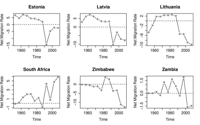
In this section we focus on six selected countries—Estonia, Latvia, Lithuania, South Africa, Zimbabwe, and Zambia—to highlight the need for regularization of the correlation matrix.
Migration rates in Estonia, Latvia, and Lithuania over the period from 1950 to 2010 look quite similar (top row of Figure 1.) All three countries share a spike in out-migration during the 1990–1995 time period, which appears as a large negative forecast error in a first-order autoregressive (AR(1)) model. This sudden jump in out-migration among the Baltic states shares a common cause, namely the fall of the Soviet Union, which both induced westward migration and prompted many ethnic Russians to return to Russia (Fassmann and Munz, 1994; Okólski, 1998)
Meanwhile, several countries in Southern Africa also experienced big shifts in migration rates during the 1990–1995 time period (bottom row of Figure 1.) From 1990 to 1995, South Africa received substantially more in-migration than it had in previous decades, while Zimbabwe and Zambia both switched from being net receivers of migrants to net senders. For these three countries, at least some of the change in migration was due to political shifts related to the end of South Africa’s apartheid policy. For example, the number of legal entrants to South Africa who overstayed their visas grew dramatically during the 1990s, with many such entrants coming from other countries of the Southern African Development Community (Crush, 1999).
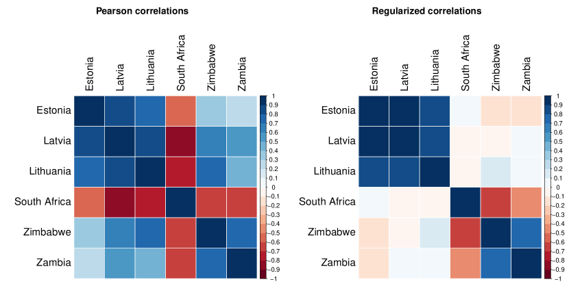
Because all six countries experienced pronounced changes in migration rates during the same time period, the usual Pearson estimates of the correlation in forecast errors are relatively large for these six countries (left panel of Figure 2.) Knowledge of world affairs, however, suggests that some of these correlations may be spurious. There are plausible explanations for the correlations within the three Baltic nations and within the Southern African nations, but the cross-regional correlations are suspect. In fact, the cross-regional correlations seem to have arisen largely from a coincidental synchrony in the timing of disparate geopolitical events, and do not represent correlations that we would expect to continue to exist in future migration data. Our method is designed to shrink these seemingly spurious cross-regional correlations, producing the estimated correlation matrix shown in the right panel of Figure 2. Cross-regional correlations decrease substantially in magnitude, while correlations within regions remain largely unchanged.
1.2 Background
Country-specific projections of international migration are an important input in policy-making decisions (Bijak et al., 2007; Brown and Bean, 2012). Projected migration figures are commonly used in long-term planning of social welfare programs (U.S. Social Security Administration, 2013; Wright, 2010). However, projection of migration is difficult—Bijak and Wiśniowski (2010) describe migration as “barely predictable”—and global modeling of migration remains somewhat rudimentary. The United Nations Population Division produces global projections of fertility, mortality, and migration for all countries (United Nations, 2012). For most countries, the 2012 revision of the World Population Prospects (WPP) deterministically projects net migration to persist at current levels until 2050 and decline linearly thereafter.
To produce fully probabilistic population projections, one must incorporate probabilistic projections of fertility and mortality with a global probabilistic model of migration. It follows from the demographic balancing equation that the contribution of migration to population change is given by net migration (that is, in-migration minus out-migration.) Probabilistic models exist for both net migration (Azose and Raftery, 2015; Azose et al., 2016) and in- and out-migration separately (Wiśniowski et al., 2015). Both of these models are Bayesian hierarchical autoregressive models which treat forecast errors in migration as independent across countries, conditional on model parameters. This leads to projections that are well calibrated for individual countries, but may not be for multi-country aggregates. Our method aims to relax this independence assumption.
It is worth noting that a strong correlation in migration rates themselves need not translate to a strong correlation in forecast errors. For example, from 1960 through 2000, Mexico was consistently either the largest or second-largest source of migration flows to the US, with nearly 5 million Mexicans migrating to the US during the 1990’s (Abel, 2013). While we estimate that net migration rates for the USA and Mexico have a correlation of -0.56 based on quinquennial WPP data from 1950-2010, we estimate a correlation in forecast errors of only -0.07. That is, most of the relationship between the USA and Mexico is already captured by the autoregressive model parameters, and the “random” components of migration rates for the two countries are nearly independent conditional on the AR(1) model.
In this high-dimensional setting with short time series, the empirical correlation matrix is a poor estimator, in that it can include many spuriously large estimated correlations. Our goal is to use regularization to improve an empirical correlation matrix for forecast errors in migration. There is a large body of literature on regularized estimation of covariance matrices, with applications in genomics, image processing, and finance, among other fields (Fan et al., 2014). The novelty of our method is that it allows the incorporation of available prior information in an easily interpretable way.
Existing covariance estimators based on penalized likelihood maximization are typically maximum a posteriori (MAP) estimates under some prior belief about covariance, but these formulations are not well suited to specifying beliefs directly about elements of the correlation matrix. Perhaps the most similar method to ours is that of Bien and Tibshirani (2011), which allows informative priors on elements of the covariance matrix rather than the correlation matrix. Their method is not directly applicable to our setting, as our goal is to augment existing marginal variances with a suitable correlation structure. Other proposed MAP estimators include the graphical lasso (Friedman et al., 2008), which can be used to place an informative prior on the inverse covariance, and the method of Chi and Lange (2014), which penalizes covariance estimates that have very large or very small eigenvalues. An extreme example is given by Chaudhuri et al. (2007), who provide a method for covariance estimation in the presence of known zeroes. Zhang and Zou (2012) propose a variant on penalized likelihood maximization that replaces the negative log-likelihood with a simpler loss function.
A related class of covariance estimators relies on shrinkage of an empirical covariance matrix towards a simpler estimator, typically trading some bias for lower mean squared error (Ledoit and Wolf, 2003, 2004, 2012). A strength of these methods is that so long as the empirical covariance matrix is positive semi-definite and the shrinkage target is positive definite, a linear combination of the two will naturally be positive definite. Applying a shrinkage method to the migration setting would be difficult, as the elements we would like to penalize do not define a positive definite shrinkage target.
A form of regularization that is straightforward to implement is applying thresholding directly to elements of a covariance or correlation matrix (Bickel and Levina, 2008a; El Karoui, 2008); these authors show that a hard-thresholded covariance matrix is consistent in operator norm. Generalized thresholding (Antoniadis and Fan, 2001), developed in the context of wavelet applications, provides a class of related regularized estimators. A key difficulty with such estimators is that care must be taken to ensure that the resulting estimator is positive definite. In some problems, this can be handled by selecting a thresholding constant from an appropriate range (Fan et al., 2013). Unfortunately, such an approach is not easily adapted to our problem. The structure of the elements we wish to penalize is such that we can tolerate only a small amount of shrinkage of all penalized elements before our estimated correlation matrix loses positive definiteness.
One fully Bayesian treatment is proposed by Liechty et al. (2004), who include substantive prior information by specifying clusters of correlations which they expect to be similar. This is unfortunately unsuitable to our setting, since geographical and cultural proximity can give rise to either positive or negative correlations. Huang et al. (2013) describe a computationally attractive non-informative prior on covariances which does not easily extend to the informative priors we would like to include. Other fully Bayesian treatments are given by Barnard et al. (2000), who propose a prior on the correlation matrix which is either marginally or jointly uniform, and Leonard and Hsu (1992) and Deng and Tsui (2013), who propose Bayesian estimation of the logarithm of the covariance matrix, which is unfortunately hard to interpret.
In scenarios where there is a natural ordering to the variables, it is often reasonable to make the assumption that large values of imply near independence or conditional independence. When this is the case, one can regularize by banding or tapering of the covariance or inverse covariance matrix (Bickel and Levina, 2008b; Fan et al., 2007; Furrer and Bengtsson, 2007; Chen et al., 2013; Levina et al., 2008). These approaches are not suitable to our problem, as there is no natural ordering of countries.
2 Methods
We start with an established, well-calibrated autoregressive model on net migration rates for all countries (Azose and Raftery, 2015). This model has the form:
| (1) | ||||
| (2) | ||||
| (3) | ||||
| (4) | ||||
| (5) |
Notationally, is a length- vector of net migration rates for all countries during the time period from to , where is the number of countries analyzed. The quantities , , and are vectors of model parameters, and is a length- vector of zeroes. (We have omitted here the specifics of hyperpriors on , , , and , which Azose and Raftery selected to reflect the ranges of plausible values.) Notably, forecast errors in their model are treated as independent, conditional on the model’s other parameters. Our method augments this model with an estimated correlation structure. Although this paper focuses on the migration context, the same technique could be applied to probabilistic models of other demographic indicators.
From this point forward, we refer to Azose and Raftery’s model as the Bayesian Hierarchical Model with Independent Forecast Errors (BHM+IFE). In principle, the methodology we describe here provides a means of estimating a correlation matrix to be adjoined to any probabilistic model with conditionally independent forecast errors.
The outline of our procedure for estimating a correlation matrix is as follows:
-
1.
From the BHM+IFE model, draw a posterior sample of realizations of model parameters, , , , …, , , .
-
2.
Convert the estimated forecast errors from the posterior sample of model parameters to a single empirical correlation matrix, .
-
3.
Combine the empirical correlation matrix with informative priors on correlations to obtain a maximum a posteriori (MAP) correlation estimate, .
This procedure can be viewed as performing a single step of the Monte Carlo EM (MCEM) algorithm (Wei and Tanner, 1990).
The posterior sampling in stage 1 can be performed using any reasonable sampling procedure. In practice, we performed our posterior sampling with a combination of Gibbs sampling and Metropolis-Hastings steps.
In the following sections, we first discuss the details of obtaining an MAP estimator (Section 2.1) and then the question of what to use for an empirical correlation matrix (Section 2.2). This is followed by an algorithm for computing the MAP estimator (Section 2.3), and finally discussion of a criterion for selecting a regularization parameter (Section 2.4).
2.1 MAP correlation estimate
Our goal is to estimate the correlation structure, , of forecast errors, . We assume a model of the form
| (6) |
where the variance matrix, , decomposes into standard deviations, , and a correlation matrix, , as . To determine a MAP estimator for , we express the posterior distribution for as a product of likelihood and prior.
2.1.1 Data Likelihood
Equation (6) implies a likelihood function for of the form
| (7) |
restricted to the space of valid correlation matrices (i.e. positive semi-definite matrices with ones on the diagonal.) Matrix trace identities simplify this likelihood to
| (8) |
where
| (9) |
The evidence from the data is encapsulated in , which is something akin to an empirical correlation matrix. Note that would be a sufficient statistic for if the ’s and were known. In fact neither the ’s nor are known, and must be replaced with a sensible estimate in order to proceed. Details of the estimation of are given in Section 2.2.
2.1.2 Prior
Our choice of prior distribution on is motivated by a desire to incorporate informative prior beliefs about which country pairs are likely to be nearly uncorrelated. As such, we choose a prior of the form
| (10) |
again restricted to . The matrix with entries is a penalty matrix that encodes the extent to which we believe that countries and may be correlated. In our application to migration, we constrain all the entries in to be equal to 0 or 1, although in general may be allowed to have arbitrary non-negative entries. The parameter is an overall regularization parameter that encodes how strongly we want to penalize correlations.
The key benefit of this prior is its ease of interpretability. Setting expresses a belief that should be close to zero, with the strength of that belief controlled by . Setting implies that all values of are equally believable, a priori. Other penalized likelihood estimators have been proposed, corresponding to MAP estimators under implied priors on precision (Friedman et al., 2008), covariance (Bien and Tibshirani, 2011), or eigenvalues of the covariance matrix (Chi and Lange, 2014). None of these allow one to specify prior beliefs about correlations directly.
Note that under this specification, the prior distribution of the correlation is either uniform or truncated Laplace conditional on the rest of the correlation matrix, but marginal distributions will not be uniform or double exponential. Although it is possible to specify a marginally uniform prior on all elements of the correlation matrix (Barnard et al., 2000), we know of no way to specify a distribution that is marginally uniform for some elements and marginally peaked at zero for others.
Because the prior density is a product of Laplace densities on correlations, we will refer to our eventual correlation estimator as the LPoC (Lapalace Prior on Correlations) estimator. Augmenting the BHM+IFE with the LPoC correlation estimate produces the BHM+LPoC model.
2.1.3 Posterior
Combining the likelihood and prior, we obtain the log posterior distribution for , equal to
| (11) |
where denotes elementwise matrix multiplication, and gives the sum of the absolute value of the elements of a matrix.
Thus, finding the MAP estimator for is equivalent to solving the minimization problem
| (12) |
Algorithmic details of a numerical solution are given in Section 2.3.
Note that if the penalty parameter, , is zero, then this minimization problem yields the maximum likelihood estimator (MLE) of R conditional on . So long as is itself positive definite, this MLE is just , the empirical correlation matrix. Similarly, if is held fixed as grows, the penalty term in (12) goes to zero and the LPoC estimator converges to . Since is consistent for , the LPoC estimator is also consistent.
2.2 Estimating
Since the forecast errors and model parameters of the BHM+IFE model are unknown, we do not have access to the true value of . Instead we use an estimate of . For practical reasons, we would prefer to have itself be a valid correlation matrix so that (12) will have a known analytic solution in the limiting scenarios where grows or goes to zero. Accordingly, we might choose an estimator with elements defined by
| (13) |
where is the posterior mean of from the BHM+IFE model. This estimate, , is the MLE for estimating the correlation matrix of a multivariate normal random variable with mean known to be zero and unknown marginal variance terms. By construction, is guaranteed to be positive semi-definite and to have ones on the diagonal.
However, in our application, is low rank, since is small relative to the dimension of the matrix. For computational reasons, we would prefer to have a strictly positive definite matrix, so we estimate by
| (14) |
This change can be viewed as augmenting our estimates of with a small amount of additional uncorrelated data.
2.3 Solving the minimization problem
We apply a majorize-minimize algorithm similar to that used by Bien and Tibshirani (2011) to the minimization problem in (12). The function being minimized over is the sum of a convex and a concave component. The majorize-minimize algorithm repeatedly iterates through the following steps:
-
1.
Replace the concave component with its tangent plane to obtain a fully convex function.
-
2.
Find the global minimum of the convex function from Step 1.
-
3.
Update the estimate of the tangent plane.
Notationally, we label our starting point for this algorithm as and subsequent iterations of this majorize-minimize algorithm are denoted with subscripts .
In (12), the concave component is , which we replace with the tangent plane . After simplifying and removing terms which are constant in , the convex minimization problem in the th iteration of the algorithm is
| (15) |
Now all of the terms the objective function in (15) are convex, and all but are differentiable, so we can apply the generalized gradient descent algorithm (Beck and Teboulle, 2009). Each generalized gradient descent step takes the form
| (16) |
If the restriction to were not present, this problem would have a simple analytic solution, given by
| (17) |
where is the element-wise soft-thresholding operator defined by
| (18) |
(This move is actually restricted to the off-diagonal elements only, as the diagonal elements of a correlation matrix are constrained to equal 1.) Thus, if there were no positive definiteness constraint, each update step would consist of a gradient descent step according to the gradient of the differentiable component followed by soft-thresholding the result.
Although we do have to satisfy a positive definiteness constraint, we can start by trying the update step in (17). If this update results in a valid correlation matrix, then that matrix is our solution to (16), and we replace with . However, sometimes the soft-thresholded gradient step results in a matrix that is not positive definite. In that case, it is possible to appeal to a slower, iterative solution to (16). One such solution is given by Cui et al. (2016). In practice, as long as we are looking for a solution in the interior of , it is good enough to simply reduce step size rather than appealing to the relatively costly iterative algorithm whenever the generalized gradient descent suggestion lies outside of .
Step size selection has a large impact on performance and convergence of this algorithm. Details of step size selection are discussed in Appendix A.
2.4 Selecting the regularization parameter
Although the penalty matrix can be selected on the basis of world knowledge, we are less likely to have genuine prior beliefs about the value of the regularization parameter . Accordingly, we need some procedure for selecting a value for . In regularization problems, it is common to select the regularization parameter via cross-validation (Bien and Tibshirani, 2011; Chi and Lange, 2014; Huang et al., 2006). This approach is too computationally intensive to be feasible for our application. Among shrinkage estimators, it is common to choose the amount of shrinkage in order to minimize an expected loss function (James and Stein, 1961; Ledoit and Wolf, 2003). However, no suitable analytic result exists that allows us to approximately minimize expected loss in our scenario.
Consequently, we developed a heuristic criterion that selects in a way that aligns with the goal of our regularization process. Our method’s intent is to shrink the magnitude of penalized elements of the correlation matrix while leaving unpenalized elements more or less unchanged. In practice, although we succeed at bringing penalized elements towards zero, this shrinkage usually comes at the cost of inflating other elements. We have observed that this inflation tends to grow more pronounced as grows. For very large values of , our estimated correlation matrix may shrink nearly all penalized entries to zero at the expense of inflating a few elements (both penalized and unpenalized) to nearly . This is not a desirable outcome.
Although it may seem counterintuitive at first, the observed inflation is not an artifact of a coding error or poor convergence of our algorithm. A simple reproducible example of inflation in a matrix is provided in Appendix B. In this low-dimensional setting, standard numerical optimization routines agree with the results from our code and both display inflation of unpenalized elements.
Our criterion for selecting compares the off-diagonal elements of and . We choose the value of which maximizes the difference between average shrinkage and average inflation. Formally, our criterion is defined by
| (19) |
Large positive values of are desirable, as they correspond to values of for which we induce a lot of shrinkage and not much inflation.
3 Results
In this section, we first report results from applying our method to global migration data in Section 3.1. Section 3.2 then provides a simulation study which demonstrates that our method outperforms Pearson correlations and the Ledoit-Wolf shrinkage estimator (Ledoit and Wolf, 2003) in the scenario where the penalty matrix is appropriate to the true correlation structure.
3.1 Application to migration
3.1.1 Data
We use data on net migration from the 2012 revision of the World Population Prospects (WPP) United Nations (2012). The WPP contains estimates of net migration for all countries in five-year time periods from 1950 until 2010, a total of 12 time periods. We compute the net migration rate as the net number of migrants in country over the five year period starting at time , divided by thousands of individuals in country at time .
Because we want to express prior beliefs as a function of distance covariates, we restrict the set of modeled countries to the 191-country overlap between the WPP 2012 and the set of countries included in CEPII’s GeoDist database, a database of bilateral distance covariates defined on pairs of countries (Mayer and Zignago, 2011).
3.1.2 Selection of
Our estimation technique requires that we choose a penalty matrix, , that reflects our prior beliefs about which country pairs are likely to be correlated. Although it would be possible to elicit expert opinion about each of the roughly 18,000 country pairs, we instead choose a that can be characterized in terms of just a few covariates. Our matrix penalizes a pair of countries if none of the following conditions is met:
-
1.
The two countries are contiguous.
-
2.
The two countries’ most important cities are located less than 3000 km apart.
-
3.
The two countries are in the same region according to the United Nations Population Division’s division of the world into 22 regions, based on both geographical contiguity and cultural affinity (United Nations, 2012).
-
4.
The two countries are currently in a colonial relationship.
This definition of is in line with migration theory, which suggests that migrant flows are more likely when monetary and social costs of movement are low (Harris and Todaro, 1970; Lee, 1966; Sjaastad, 1962; Stark and Bloom, 1985), as will be the case with countries which are geographically proximate or share administrative ties. This definition penalizes 85% of country pairs, leaving 15% unpenalized. The average country is considered to be “close” to 29 other countries, and “distant” from the remaining 161.
In selecting these conditions, we examined nine candidate distance covariates. The first eight such covariates come from CEPII’s GeoDist database (Mayer and Zignago, 2011), while the ninth is derived from the United Nations division into 22 regions. The left column of Table 1 gives the complete list of covariates considered. As an empirical basis for determining which criteria to include in defining our penalty matrix, we examined the elements of the sample correlation matrix for all pairs of countries meeting each criterion. Using a Kolmogorov-Smirnov test, we tested whether the distribution of these sample correlations was different from the distribution of elements of the sample correlation matrix under a null hypothesis of uncorrelated errors. The right column of Table 1 shows the -values from these Kolmogorov-Smirnov tests. Our definition of the penalty matrix includes all covariates with a -value less than 0.05.
| Covariate | -value |
|---|---|
| Contiguous | 0.019 |
| Common language (official) | 0.23 |
| Common language (spoken by 9% of pop.) | 0.58 |
| Geodesic distance less than 3000 km | 0.0003 |
| Colonial relationship after 1945 | 0.57 |
| Common colonizer after 1945 | 0.11 |
| Current colonial relationship | 0.035 |
| Ever had a colonial link | 0.36 |
| Same UN Region | 0.036 |
3.1.3 Selection of the regularization parameter,
We computed values of for all values of from 0 to 3 in increments of 0.1. Figure 3 shows the value of over a range of values. We found that peaked at , where we find average shrinkage of 0.13 compared with average inflation of 0.07. Increasing from 0.6 to 0.7 induces additional shrinkage, but at the cost of greatly inflating some correlations. Accordingly, we choose as our estimate of .

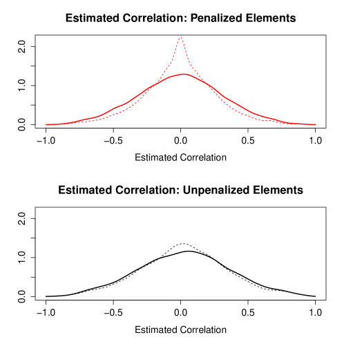
Figure 4 shows the impact of regularization on the correlation matrix. Among penalized elements (top panel), we see significant shrinkage towards zero, although many penalized elements remain large in magnitude, even after regularization. The bottom panel shows the unpenalized elements of the correlation matrix before regularization (solid curve) and after (dashed curve). On average we induce some shrinkage in the unpenalized elements, but the distribution is largely unchanged.
3.1.4 Projection and evaluation
We augment the BHM+IFE model with the LPoC estimate to produce probabilistic projections of migration for any collection of countries. Figure 5 contains medians and 80% prediction intervals of projected migration for all continents. In Africa, negative correlations narrow our projections. In Europe, positive correlations cause forecasts to widen. For the other continents, we see little change in projected migration.

For evaluation, we compare true migration rates for regional aggregates in 1995–2010 with projections of the same regional aggregates based only on migration data from 1950–1995. This procedure entails re-estimation of the BHM+IFE model using only the 1950–1995 data, followed by construction of an empirical correlation matrix, selection of , and extraction of . We compare the performance of the BHM+IFE model on regional aggregates to a model using the same sampled values of , , and , but augmented with .
As an evaluation metric, we use the negatively oriented continuous ranked probability score (CRPS) (Hersbach, 2000; Gneiting and Raftery, 2007). The CRPS compares the cumulative distribution function, , of a probabilistic forecast to an observation, , and is defined by
| (20) |
In our application the two probabilistic forecasts under consideration have the same mean as one other, by design. One approximate way of looking at CRPS in this setting is that when is close to the mean of the forecast, we reward for having low variance; when is far from the mean, we reward for having high variance.
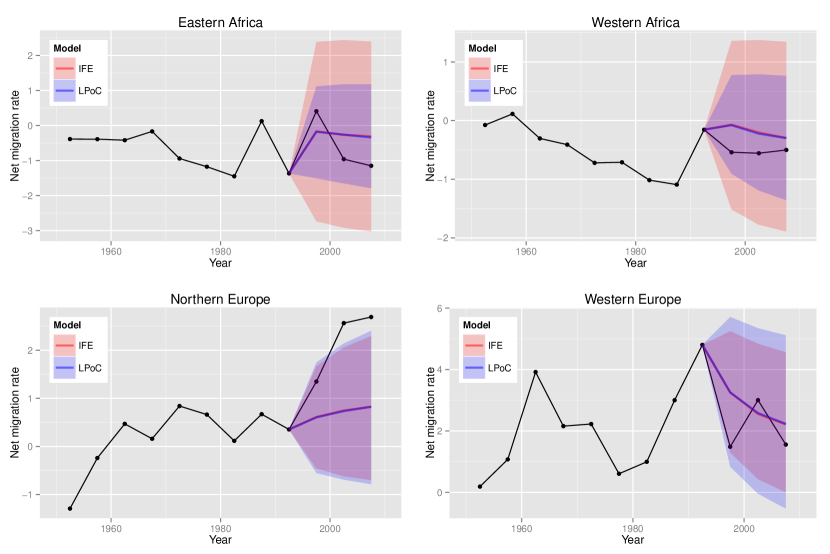
Table 2 gives CRPS for projections of aggregate migration for the six continents. Our model improves the quality of projections in Africa and Europe, while projections for the other four continents are more or less unchanged. Figure 6 illustrates the change in projections of net migration in 1995–2010 for four subregions of Africa and Europe. Projections from the BHM+IFE model are in red; projections from BHM+LPoC are in blue. Our method narrows prediction intervals in Eastern and Western Africa, bringing the width of the 80% prediction intervals more into line with the range of observed variability. In both regions, true migration rates for the projected period stayed within our narrower intervals. In contrast, our method widens projections in Northern and Western Europe, where the 80% intervals from the BHM+IFE model either miss or nearly miss capturing some of the observed data points.
| IFE | LPoC | |
|---|---|---|
| Africa | 1.66 | 1.49 |
| Asia | 0.73 | 0.74 |
| Europe | 3.92 | 3.76 |
| Latin America and the Caribbean | 1.62 | 1.62 |
| Northern America | 5.02 | 4.99 |
| Oceania | 8.53 | 8.49 |
3.2 Simulation study
In this section we show by simulation that our regularization procedure improves correlation estimates in a low-dimensional setting. To match the application of interest, we simulate 12 observed time points from an AR(1) process with correlated errors. For computational tractability, we decrease the number of simulated countries from 191 in the real data to 9 in the simulation. For each of 100 simulations, we perform the following procedure:
-
1.
Generate a set of simulated migration rates from an AR(1) process with errors correlated as described below.
-
2.
Produce point estimates of via MCMC sampling of , , and .
-
3.
Convert ’s to a matrix using the procedure in Section 2.2.
-
4.
Solve the minimization problem (12) to obtain a regularized estimate for the correlation matrix.
Since the procedure for selecting is computationally intensive, we perform this procedure only once and use the same value of for all subsequent simulations.
3.2.1 Simulation details
We simulate a collection of nine countries with true migration rates governed by the AR(1) process
| (21) |
For simplicity we take , , and
| (22) |
We fix to be block diagonal. Compound symmetric correlation structure within each block is given by
| (23) |
and the full covariance matrix by
| (24) |
We then simulate observations and attempt to make inference on the correlation structure of .
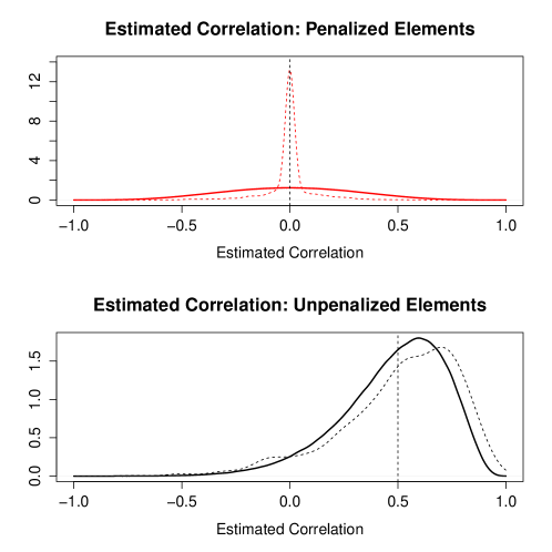
Because we are basing inference on a small number of time points, Pearson estimates of correlation are highly variable. Solid curves in Figure 7 show the distributions of the off-diagonal elements of the unregularized Pearson correlation matrix in the ideal scenario where the values of can be perfectly estimated. The top panel shows the distribution of the elements for which the true correlation is zero. The bottom panel shows elements for which the true correlation is 0.5. In both cases, high variability makes inference difficult. Our method is designed to decrease variability among estimated correlations for those country pairs where prior knowledge suggests that correlation should be close to zero.
To illustrate a best case scenario, we choose a penalty matrix which is well suited to the true correlation structure. The simplest such is the one which penalizes the off-diagonal elements of the correlation matrix if and only if the true correlation is zero. That is given by
| (25) |
3.2.2 Initial run to select
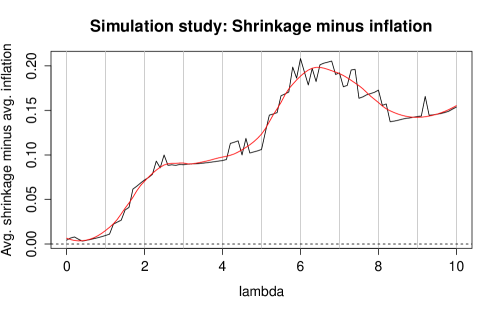
Our procedure to select is computationally expensive, as it requires us to compute repeatedly as varies. We therefore perform this procedure only once and use the same for estimation of in all subsequent simulated data sets. Figure 8 plots our -selection criterion based on a single simulated data set over the range . The exact curve, shown in black, exhibits some jumpiness in this low-dimensional setting, a problem which naturally becomes less severe in the high-dimensional setting of interest. Because of this jumpiness, we base our selection of on a Lowess-smoothed curve, selecting the maximizing value of .
3.2.3 Evaluation of repeated estimation of
We produced 100 estimates of from 100 different sets of simulated migration rates, all using the same block diagonal correlation structure. Dashed lines in Figure 7 show the distribution of off-diagonal elements of , split into those elements where the true correlation is 0 and elements where the true correlation is 0.5 (top and bottom panel, respectively).
Our method is successful in shrinking penalized elements towards zero. Among elements where the true correlation is zero, we correctly estimate an exact zero in 62% of cases in this simulation. Among unpenalized elements, our method produces estimates with slightly more variability (the standard deviation is 0.256 for Pearson correlations versus 0.272 for our estimates). Both methods produce estimates for unpenalized elements that are within two standard errors of the true mean value of 0.5. The mean estimated correlation is 0.489 for Pearson correlations (standard error 0.009) versus 0.514 for our estimates (standard error of 0.009). On the whole, the LPoC estimator greatly improves estimates of penalized elements at the expense of slightly increasing variability in unpenalized elements.
Table 3 compares mean absolute error and mean squared error from our method with two competing estimators. We compare our results against both Pearson correlation matrices and correlation matrices that have been regularized using the Ledoit-Wolf method, which shrinks Pearson estimates towards a spherical correlation structure (Ledoit and Wolf, 2003). In the top panel, we estimate with a Bayesian hierarchical model, as is done in our real application to migration. In the bottom panel, we assume instead a scenario where we have direct access to , as would be suitable in other applications where the interest is in estimating correlations of directly observed quantities. In both cases, our method provides an overall reduction in mean squared error by at least two thirds when compared against the Pearson sample correlation matrix. A large reduction in error from shrinking penalized elements is offset by a mild increase in error among unpenalized elements. We also outperform the Ledoit-Wolf estimator in terms of overall error.
| Values of estimated with MCMC | |||
|---|---|---|---|
| Estimator | MAE | MSE | |
| All elements | Pearson | 0.253 | 0.098 |
| Ledoit-Wolf | 0.193 | 0.055 | |
| LPoC | 0.090 | 0.028 | |
| True correlation = 0 | Pearson | 0.270 | 0.109 |
| Ledoit-Wolf | 0.190 | 0.053 | |
| LPoC | 0.049 | 0.012 | |
| True correlation = 0.5 | Pearson | 0.201 | 0.066 |
| Ledoit-Wolf | 0.200 | 0.060 | |
| LPoC | 0.214 | 0.074 | |
| True values of used | |||
| Estimator | MAE | MSE | |
| All elements | Pearson | 0.227 | 0.079 |
| Ledoit-Wolf | 0.182 | 0.047 | |
| LPoC | 0.078 | 0.022 | |
| True correlation = 0 | Pearson | 0.244 | 0.089 |
| Ledoit-Wolf | 0.162 | 0.039 | |
| LPoC | 0.041 | 0.010 | |
| True correlation = 0.5 | Pearson | 0.176 | 0.051 |
| Ledoit-Wolf | 0.243 | 0.073 | |
| LPoC | 0.190 | 0.058 | |
4 Discussion
Our method augments probabilistic projections of migration that are well-calibrated for individual countries, with a correlation structure that reflects prior knowledge of between-country correlations. By combining a high-dimensional empirical correlation matrix with an informative prior that shrinks spurious correlations, we produce an estimated correlation matrix that is in line with migration theory and improves projections of regional aggregates. When compared with a simple model that assumes uncorrelated forecast errors, our method narrows projections of net migration for Africa and widens projections for Europe. Out-of-sample evaluation confirms that these changes produce better probabilistic forecasts as measured by continuous ranked probability score. Mechanically, the novelty of our method is our prior on correlations, which benefits from being interpretable and simple in form, and converts MAP estimation to an -penalized regularization problem which is computationally tractable.
Our analysis focuses on modeling net migration, but an attractive alternative would be to model a full matrix of bilateral migration flows. Such a model would naturally imply correlations in migration—if out-migrants from country tend to go to country , then net migration in countries and will be negatively correlated. However, modeling the global bilateral flow matrix is currently not feasible. Flows are hard to estimate, even in countries with good data (De Beer et al., 2010; Raymer et al., 2011). Abel (2013) produces global estimates of migration flows based on migrant stock data, but for only a small number of time periods at which migrant stock data exist. His method involves minimizing the total number of migrants subject to the available data on migrant stocks. This induces many structural zeroes in his estimates, making modeling difficult. Because of the lack of good data on migration flows, we choose instead to work with net migration rates.
Although our method produces a MAP estimator in the presence of informative priors, we are not able to leverage any of the usual Bayesian machinery to produce a sample from the posterior distribution. While it would in theory be possible to use MCMC methods to produce a posterior sample by updating one element of the correlation matrix at a time, an updating procedure would need to iterate through some 18,000 elements of the correlation matrix, checking for positive definiteness after each proposed step. Such an algorithm is therefore likely to move around the parameter space too slowly to be of any use. In some settings a Laplace approximation centered at the posterior mode can provide a good approximation of marginal posterior distributions (Tierney and Kadane, 1986). However, the double-exponential priors in our setting render this procedure impracticable. Within each orthant of the parameter space, a quadratic approximation to the log likelihood is reasonable, but because of the penalty term, a different quadratic approximation is required for each of the roughly orthants, which is not feasible.
Given our interest in combining data with prior beliefs, an inverse Wishart prior on covariance is tempting because it allows easy sampling from the full posterior. However, the inverse Wishart distribution is restrictive in form (Barnard et al., 2000) and does not provide a straightforward way to describe prior beliefs about correlations.
Another tempting alternative is that of Liu et al. (2014), who give a simple thresholding method for producing a penalized correlation matrix that is guaranteed to be positive definite. Their estimator solves
| (26) |
to produce an estimator among the set of valid correlation matrices with minimum eigenvalue no smaller than . Although the weight matrix, , is in principle arbitrary, they use to induce greater shrinkage where empirical correlations are weakest, not as a means of conveying prior information. We would be hesitant to replace with our penalty matrix , as that off-license use of their method would not incorporate prior information in a principled way.
Our method can be generalized to shrink estimated correlations towards non-zero values by replacing the penalty term with for some target matrix . This may be desirable in cases where heavily structured estimates of correlations are available, as is the case for modeling of fertility (Fosdick and Raftery, 2014).
References
- Abel (2013) Abel, G. (2013). Estimating global migration flow tables using place of birth data. Demographic Research, 28:505–546.
- Antoniadis and Fan (2001) Antoniadis, A. and Fan, J. (2001). Regularization of wavelet approximations. Journal of the American Statistical Association, 96(455):939–955.
- Azose and Raftery (2015) Azose, J. J. and Raftery, A. E. (2015). Bayesian probabilistic projection of international migration. Demography, 52(5):1627–1650.
- Azose et al. (2016) Azose, J. J., Ševčíková, H., and Raftery, A. E. (2016). Probabilistic population projections with migration uncertainty. Proceedings of the National Academy of Sciences. Published ahead of print May 23, 2016, doi: 10.1073/pnas.1606119113.
- Barnard et al. (2000) Barnard, J., McCulloch, R., and Meng, X.-L. (2000). Modeling covariance matrices in terms of standard deviations and correlations, with application to shrinkage. Statistica Sinica, 10(4):1281–1312.
- Beck and Teboulle (2009) Beck, A. and Teboulle, M. (2009). A fast iterative shrinkage-thresholding algorithm for linear inverse problems. SIAM Journal of Imaging Sciences, 2(1):183–202.
- Bickel and Levina (2008a) Bickel, P. J. and Levina, E. (2008a). Covariance regularization by thresholding. The Annals of Statistics, 36(6):2577–2604.
- Bickel and Levina (2008b) Bickel, P. J. and Levina, E. (2008b). Regularized estimation of large covariance matrices. The Annals of Statistics, 36(1):199–227.
- Bien and Tibshirani (2011) Bien, J. and Tibshirani, R. J. (2011). Sparse estimation of a covariance matrix. Biometrika, 98(4):807.
- Bijak et al. (2007) Bijak, J., Kupiszewska, D., Kupiszewski, M., Saczuk, K., and Kicinger, A. (2007). Population and labour force projections for 27 European countries, 2002–2052: Impact of international migration on population ageing. European Journal of Population, 23(1):1–31.
- Bijak and Wiśniowski (2010) Bijak, J. and Wiśniowski, A. (2010). Bayesian forecasting of immigration to selected European countries by using expert knowledge. Journal of the Royal Statistical Society: Series A (Statistics in Society), 173(4):775–796.
- Brown and Bean (2012) Brown, S. K. and Bean, F. D. (2012). Population growth. In Gans, J., Replogle, E. M., and Tichenor, D. J., editors, Debates on U.S. Immigration. SAGE, Thousand Oaks, California.
- Chaudhuri et al. (2007) Chaudhuri, S., Drton, M., and Richardson, T. S. (2007). Estimation of a covariance matrix with zeros. Biometrika, 94(1):199–216.
- Chen et al. (2013) Chen, X., Xu, M., Wu, W. B., et al. (2013). Covariance and precision matrix estimation for high-dimensional time series. The Annals of Statistics, 41(6):2994–3021.
- Chi and Lange (2014) Chi, E. C. and Lange, K. (2014). Stable estimation of a covariance matrix guided by nuclear norm penalties. Computational Statistics & Data Analysis, 80:117–128.
- Crush (1999) Crush, J. (1999). Fortress South Africa and the deconstruction of Apartheid’s migration regime. Geoforum, 30(1):1–11.
- Cui et al. (2016) Cui, Y., Leng, C., and Sun, D. (2016). Sparse estimation of high-dimensional correlation matrices. Computational Statistics & Data Analysis, 93:390–403.
- De Beer et al. (2010) De Beer, J., Raymer, J., Van der Erf, R., and Van Wissen, L. (2010). Overcoming the problems of inconsistent international migration data: A new method applied to flows in Europe. European Journal of Population, 26(4):459–481.
- Deng and Tsui (2013) Deng, X. and Tsui, K.-W. (2013). Penalized covariance matrix estimation using a matrix-logarithm transformation. Journal of Computational and Graphical Statistics, 22(2):494–512.
- El Karoui (2008) El Karoui, N. (2008). Operator norm consistent estimation of large-dimensional sparse covariance matrices. The Annals of Statistics, 36(6):2717–2756.
- Fan et al. (2014) Fan, J., Han, F., and Liu, H. (2014). Challenges of big data analysis. National Science Review, 1(2):293–314.
- Fan et al. (2007) Fan, J., Huang, T., and Li, R. (2007). Analysis of longitudinal data with semiparametric estimation of covariance function. Journal of the American Statistical Association, 102(478):632–641.
- Fan et al. (2015) Fan, J., Liao, Y., and Liu, H. (2015). An overview on the estimation of large covariance and precision matrices. arXiv preprint arXiv:1504.02995.
- Fan et al. (2013) Fan, J., Liao, Y., and Mincheva, M. (2013). Large covariance estimation by thresholding principal orthogonal complements. Journal of the Royal Statistical Society: Series B (Statistical Methodology), 75(4):603–680.
- Fassmann and Munz (1994) Fassmann, H. and Munz, R. (1994). European East-West migration, 1945-1992. International Migration Review, 28(3):520–538.
- Fosdick and Raftery (2014) Fosdick, B. K. and Raftery, A. E. (2014). Regional probabilistic fertility forecasting by modeling between-country correlations. Demographic Research, 30(35):1011.
- Friedman et al. (2008) Friedman, J., Hastie, T., and Tibshirani, R. (2008). Sparse inverse covariance estimation with the graphical lasso. Biostatistics, 9(3):432–441.
- Furrer and Bengtsson (2007) Furrer, R. and Bengtsson, T. (2007). Estimation of high-dimensional prior and posterior covariance matrices in Kalman filter variants. Journal of Multivariate Analysis, 98(2):227–255.
- Gneiting and Raftery (2007) Gneiting, T. and Raftery, A. E. (2007). Strictly proper scoring rules, prediction, and estimation. Journal of the American Statistical Association, 102(477):359–378.
- Harris and Todaro (1970) Harris, J. R. and Todaro, M. P. (1970). Migration, unemployment and development: A two-sector analysis. American Economic Review, 60(1):126–142.
- Hersbach (2000) Hersbach, H. (2000). Decomposition of the continuous ranked probability score for ensemble prediction systems. Weather and Forecasting, 15(5):559–570.
- Huang et al. (2013) Huang, A., Wand, M. P., et al. (2013). Simple marginally noninformative prior distributions for covariance matrices. Bayesian Analysis, 8(2):439–452.
- Huang et al. (2006) Huang, J. Z., Liu, N., Pourahmadi, M., and Liu, L. (2006). Covariance matrix selection and estimation via penalised normal likelihood. Biometrika, 93(1):85–98.
- James and Stein (1961) James, W. and Stein, C. (1961). Estimation with quadratic loss. In Proceedings of the Fourth Berkeley Symposium on Mathematical Statistics and Probability, volume 1, pages 361–379.
- Ledoit and Wolf (2003) Ledoit, O. and Wolf, M. (2003). Improved estimation of the covariance matrix of stock returns with an application to portfolio selection. Journal of Empirical Finance, 10(5):603–621.
- Ledoit and Wolf (2004) Ledoit, O. and Wolf, M. (2004). A well-conditioned estimator for large-dimensional covariance matrices. Journal of Multivariate Analysis, 88(2):365–411.
- Ledoit and Wolf (2012) Ledoit, O. and Wolf, M. (2012). Nonlinear shrinkage estimation of large-dimensional covariance matrices. The Annals of Statistics, 40(2):1024–1060.
- Lee (1966) Lee, E. S. (1966). A theory of migration. Demography, 3(1):47–57.
- Leonard and Hsu (1992) Leonard, T. and Hsu, J. S. (1992). Bayesian inference for a covariance matrix. The Annals of Statistics, 20(4):1669–1696.
- Levina et al. (2008) Levina, E., Rothman, A., Zhu, J., et al. (2008). Sparse estimation of large covariance matrices via a nested lasso penalty. The Annals of Applied Statistics, 2(1):245–263.
- Liechty et al. (2004) Liechty, J. C., Liechty, M. W., and Müller, P. (2004). Bayesian correlation estimation. Biometrika, 91(1):1–14.
- Liu et al. (2014) Liu, H., Wang, L., and Zhao, T. (2014). Sparse covariance matrix estimation with eigenvalue constraints. Journal of Computational and Graphical Statistics, 23(2):439–459.
- Mayer and Zignago (2011) Mayer, T. and Zignago, S. (2011). Notes on CEPII’s distances measures: The GeoDist database.
- Nocedal and Wright (2006) Nocedal, J. and Wright, S. (2006). Numerical Optimization. Springer Science & Business Media.
- Okólski (1998) Okólski, M. (1998). Regional dimension of international migration in Central and Eastern Europe. Genus, 54(1):11–36.
- Pourahmadi (2011) Pourahmadi, M. (2011). Covariance estimation: The glm and regularization perspectives. Statistical Science, 26(3):369–387.
- Raymer et al. (2011) Raymer, J., de Beer, J., and van der Erf, R. (2011). Putting the pieces of the puzzle together: Age and sex-specific estimates of migration amongst countries in the EU/EFTA, 2002–2007. European Journal of Population, 27(2):185–215.
- Sjaastad (1962) Sjaastad, L. A. (1962). The costs and returns of human migration. Journal of Political Economy, 70(5):80–93.
- Stark and Bloom (1985) Stark, O. and Bloom, D. E. (1985). The new economics of labor migration. American Economic Review, 75(2):173–178.
- Tierney and Kadane (1986) Tierney, L. and Kadane, J. B. (1986). Accurate approximations for posterior moments and marginal densities. Journal of the American Statistical Association, 81(393):82–86.
- United Nations (2012) United Nations (2012). World Population Prospects: The 2012 Revision. United Nations, New York.
- United Nations (2015) United Nations (2015). World Population Prospects: The 2015 Revision. United Nations, New York.
- U.S. Social Security Administration (2013) U.S. Social Security Administration (2013). The 2013 Annual Report of the Board of Trustees of the Federal Old-age and Survivors Insurance and Federal Disability Insurance Trust Funds. Board of Trustees, Federal Old-Age and Survivors Insurance and Federal Disability Insurance Trust Funds.
- Wei and Tanner (1990) Wei, G. C. and Tanner, M. A. (1990). A Monte Carlo implementation of the EM algorithm and the poor man’s data augmentation algorithms. Journal of the American Statistical Association, 85(411):699–704.
- Wiśniowski et al. (2015) Wiśniowski, A., Smith, P. W., Bijak, J., Raymer, J., and Forster, J. J. (2015). Bayesian population forecasting: Extending the Lee-Carter method. Demography, 52(3):1035–1059.
- Wright (2010) Wright, E. (2010). 2008-based national population projections for the United Kingdom and constituent countries. Population Trends, 139(1):91–114.
- Zhang and Zou (2012) Zhang, T. and Zou, H. (2012). Sparse precision matrix estimation via lasso penalized D-trace loss. Biometrika, 99(1):1–18.
Appendix A Determining step size
Step size selection is necessary in high dimensions for the general gradient descent algorithm to converge quickly enough to be useful. Complex methods for step size selection are available, but we obtained reasonable results with the backtracking line search algorithm, which starts with a large step size and decreases step size whenever a proposed step results in too little improvement in the objective function.
Say we have an objective function which we are trying to minimize. The core of the backtracking line search algorithm is as follows (Nocedal and Wright, 2006).
-
1.
Fix a backtracking coefficient , a starting step size , and a starting location .
-
2.
Propose a step of length in direction . (The backtracking line search algorithm is a generic algorithm that will work regardless of how the direction is determined.)
-
3.
If the improvement in the objective function is enough to meet the Armijo condition given in (27) below, then take the proposed step. That is, take . Keep the step size constant (i.e., ).
-
4.
Otherwise, if there is any improvement in the objective function, take the proposed step, but also decrease the step size for the next iteration (specifically, set ).
-
5.
Otherwise, there must have been no improvement in the objective function. Don’t take a step, but do decrease step size. ( and .)
-
6.
Repeat steps 2-5 until convergence.
The Armijo condition, which is used to determine whether to decrease step size, is as follows. The Armijo condition is met if the following inequality is satisfied:
| (27) |
( is a constant chosen from that controls how strictly the change in must match the gradient at .)
In our application, there’s a missing component—we can’t actually compute the gradient of our objective function. The relevant objective function is given by
| (28) |
The first two terms in the sum are differentiable, but the third is not.
We rewrite the Armijo condition as
| (29) |
and then approximate with
| (30) |
Appendix B Inflation of correlation estimates
We provide here an example of our correlation estimation procedure which produces inflation in some unpenalized elements of the correlation matrix. We solved the minimization problem in (12) with three different methods, finding identical answers each time, up to small numerical tolerances. Those methods are:
-
1.
Estimate using our code, which appeals to the generalized gradient descent algorithm.
-
2.
Estimate using a black-box numerical optimization algorithm, which has access to the function we’re minimizing, but not its derivative.
-
3.
Estimate by finding an analytic expression for the gradient of the function we’re minimizing, and solve for a point where the gradient is zero.
One case in which inflation manifests if we take our evidence from the data to be given by
| (31) |
and the penalty matrix by
| (32) |
We denote the unknown true correlation matrix by
| (33) |
We fix the regularization parameter at . The problem is then to estimate the three parameters , , and .
With all three methods we find an estimate of
| (34) |
Note that the second element, which is penalized, experiences shrinkage towards zero, as expected. The first element is inflated, while the third is both inflated and changes sign.