Generalized linear sampling method for elastic-wave sensing of heterogeneous fractures
Abstract
A theoretical foundation is developed for active seismic reconstruction of fractures endowed with spatially-varying interfacial condition (e.g. partially-closed fractures, hydraulic fractures). The proposed indicator functional carries a superior localization property with no significant sensitivity to the fracture’s contact condition, measurement errors, and illumination frequency. This is accomplished through the paradigm of the -factorization technique and the recently developed Generalized Linear Sampling Method (GLSM) applied to elastodynamics. The direct scattering problem is formulated in the frequency domain where the fracture surface is illuminated by a set of incident plane waves, while monitoring the induced scattered field in the form of (elastic) far-field patterns. The analysis of the well-posedness of the forward problem leads to an admissibility condition on the fracture’s (linearized) contact parameters. This in turn contributes toward establishing the applicability of the -factorization method, and consequently aids the formulation of a convex GLSM cost functional whose minimizer can be computed without iterations. Such minimizer is then used to construct a robust fracture indicator function, whose performance is illustrated through a set of numerical experiments. For completeness, the results of the GLSM reconstruction are compared to those obtained by the classical linear sampling method (LSM).
Keywords: Generalized linear sampling method, inverse scattering, seismic imaging, elastic waves, fractures, specific stiffness, hydraulic fractures.
1 Introduction
Most recent advancements in the waveform tomography of discontinuity surfaces reside in the context of acoustic and electromagnetic inverse scattering. Spurred by the early study in [22], such developments include: i) the Factorization Method (FM) [8, 13]; ii) the Linear Sampling Method (LSM) [19, 11] and MUSIC algorithms [30, 20]; iii) the subspace migration technique [32], and iv) the method of Topological Sensitivity (TS) [18, 7, 31]. In general, the LSM and FM techniques are applicable to a wide class of interfacial conditions and inherently carry a superior localization property – potentially leading to high-fidelity geometric reconstruction. These methods, however, may suffer from the sensitivity to measurement uncertainties. In contrast the TS approach, that is inherently robust to noisy data, fails to adequately recover the shape of a scatterer at long illuminating wavelengths. The subspace migration methods offer another alternative for a high-fidelity reconstruction, even from partial-aperture data, while requiring some a priori knowledge about the geometry of a discontinuity surface. Among the aforementioned methods, the LSM has been applied to the problem of elastic-wave imaging of fractures with homogeneous (traction-free) boundary condition [9], while the TS approach was recently extended to cater for qualitative elastodynamic sensing of fractures endowed with a more general class of contact laws [5, 33]. In geophysics, major strides [36, 37, 27, 28, 17] have been made toward a robust reconstruction of fractures via seismic waveform tomography. So far the proposed methods, often reliant upon a rudimentary parameterization of the fracture geometry (e.g. planar fractures) and nonlinear minimization, entail a number of impediments including: i) high computational cost; ii) sensitivity to the assumed parametrization; iii) computational instabilities [28], and iv) major restrictions in terms of the seismic sensing configuration [17, 27], namely the location of sources and receivers relative to the (planar) fracture surface. One recent study aiming to mitigate such limitations can be found in [37] that makes use of focused Gaussian beams emitted from the surface source/receiver arrays to non-iteratively assess the orientation, spacing, and compliance of systems of parallel planar fractures.
This work aims to develop a non-iterative, full-waveform approach to 3D elastic-wave imaging of fractures with non-trivial (generally heterogeneous and dissipative) interfacial condition. To this end, the sought indicator map – targeting geometric fracture reconstruction – is preferably (i) agnostic with respect to the fracture’s interfacial condition, (ii) robust against measurement errors, and (iii) flexible in terms of sensing parameters, e.g. the illumination frequency. This is pursued by drawing from the theories of inverse scattering [12, 14] and, in particular, by building upon the Factorization Method [21, 8] and the recently developed Generalized Linear Sampling Method (GLSM) [2, 3] which completes the theoretical foundation of its LSM predecessor. First, the inverse problem is formulated in the frequency domain where the illuminating wavefield is described by the elastic Herglotz wave function [16] with its inherent compressional (P) and shear (S) wave components. On characterizing the induced scattered wavefield in terms of its far-field P- and S-wave patterns [25], the far-field operator is then defined as a map from the Herglotz densities to the far-field measurements. In this setting, the GLSM indicator functional is introduced as in [3] on the basis of (i) a custom factorization of the far-field operator, and (b) a sequence of approximate solutions to the LSM integral equation, seeking Herglotz densities whose far-field pattern matches that of a point-load solution radiating from the sampling point. The latter sequence is essentially a set of penalized least-squares misfit functionals – aimed at producing nearby solutions to the LSM equation, where the penalty term is constructed using a factorization component of . Minimizing this class of cost functionals in their most general form requires an optimization procedure [3]. Thanks to the premise of a linear contact law, however, this study takes advantage of the so-called -factorization [21, 8] of the far-field operator to formulate the penalty term. This results in a sequence of convex GLSM cost functionals whose minimizers can be computed without iterations.
2 Problem statement
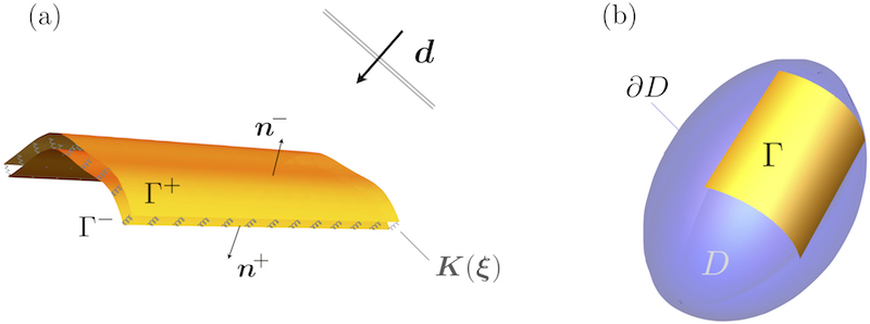
With reference to Fig. 1(a), consider the elastic-wave sensing of a partially closed fracture embedded in a homogeneous, isotropic, elastic solid endowed with mass density and Lamé parameters and . The fracture is characterized by a heterogeneous contact condition synthesizing the spatially-varying nature of its rough and/or multi-phase interface. Next, let denote the unit sphere centered at the origin. For a given triplet of vectors and such that and , the obstacle is illuminated by a combination of compressional and shear plane waves
| (1) |
propagating in direction , where and denote the respective wave numbers. The interaction of with gives rise to the scattered field , solving
| in | (2) | |||||
| on |
where is the frequency of excitation; is the jump in across , hereon referred to as the fracture opening displacement (FOD);
| (3) |
is the fourth-order elasticity tensor; denotes the th-order symmetric identity tensor; is the free-field traction vector; is the unit normal on , and represents a heterogeneous bijective contact law over the fracture surface, physically relating the displacement jump to surface traction. In many practical situations, the fracture’s contact law is linearized about a dynamic equilibrium state as
| (4) |
where is a symmetric (due to reciprocity considerations) and possibly complex-valued matrix of specific stiffness coefficients.
Remark 1.
In what follows, the analysis is based on the linear contact condition (4) over . Under the premise of bijectivity, most of the ensuing developments (except for the factorization method) can be adapted to handle nonlinear contact laws; such extension, however, is beyond the scope of this study.
The formulation of the direct scattering problem can now be completed by requiring that satisfies the Kupradze radiation condition at infinity [24]. On uniquely decomposing the scattered field into an irrotational part and a solenoidal part as where
| (5) |
the Kupradze condition can be stated as
| (6) |
uniformly with respect to .
Dimensional platform.
In what follows, all quantities are rendered dimensionless by taking , , and – the characteristic size of a region sampled for fractures – as the respective scales for mass density, elastic modulus, and length – which amounts to setting [4].
Function spaces.
To assist the ensuing analysis, the fracture surface is arbitrarily extended, as shown in Fig. 1(b), to a piecewise smooth, simply connected, closed surface of a bounded domain such that the normal vector to the fracture surface coincides with the outward normal vector to – likewise denoted by . We also assume that is an open set (relative to ) with positive surface measure. Following [26], we define
| (7) | ||||
and recall that and are respectively the dual spaces of and . Accordingly, the following embeddings hold
| (8) |
Remark 2.
In the context of fracture mechanics, it is well known that continuously as (typically as , [35] where is a normal distance to when is smooth), which lends credence to the assumption used hereon.
3 On the well-posedness of the forward scattering problem
Serving as a prerequisite for the analysis of the inverse scattering problem, this section investigates the well-posedness of the direct scattering problem (2)–(6). Let be sufficiently large so that the ball of radius contains , and consider the Dirichlet-to-Neumann operator associated with the scattering problem in , namely
where is the unique radiating solution, satisfying (6), of
| in | (9) | |||||
| on |
The scattering problem (2)–(6) can now be equivalently written in terms of as
| in | (10) | |||||
| on | ||||||
| on |
where on . This problem can be written variationally in terms of as
| (11) | ||||
where and respectively denote the and duality products that extend inner products. The analysis of the forward scattering problem is based on the following properties of the Dirichlet-to-Neumann operator (see also [10]). For clarity, we will use an abbreviated notation of relevant vector norms where e.g. is denoted by and so on.
Lemma 3.1.
There exists a bounded, non-negative and self-adjoint operator such that is compact. Moreover,
| (12) |
Proof.
Let and . Multiplying the first equation in (9) by and integrating by parts on yields
where for . Using the well-posedness of (9) and the Riesz representation theorem, we define by
On demonstrating that for some constant independent of , the compactness of then follows from the compactness of mapping (resp. ) from into (resp. ) thanks to the compact embedding of into and the standard regularity results for scattering problems [26], which can be recovered from the boundary integral representation of in in terms of boundary data on . As shown in A, the sign of the imaginary part of is a consequence of the asymptotic behavior of at infinity [24] which implies
| (13) |
The sign-definiteness of the imaginary part is a consequence of the Rellich lemma [14] applied to and , which requires that whenever . ∎
Theorem 3.2.
Assume that and that is symmetric such that on , i.e. that , and a.e. on . Then problem (11) has a unique solution that continuously depends on .
Proof.
Since , the antilinear form may be understood as a duality pairing . The continuity of this form comes from the continuity of the trace mapping from into .
On the basis of the adopted dimensional platform i.e. (see Section 2), the sesquilinear form on the left hand side of (11) can be decomposed into a coercive part
| (14) |
and a compact part
| (15) |
The coercivity of follows from the Korn inequality [26] and the non negative sign of (Lemma 3.1). Now, in order to prove that the antilinear form B defines a compact perturbation of , one may observe that
for a constant independent of and . The claim then follows from Lemma 3.1, the compact embedding of into and the compactness of the trace operator as an application from into where the latter comes from the compact embedding of into .
4 Elements of the inverse scattering solution
This section is devoted to the introduction of the far-field operator – relevant to the scattering problem (2), and the derivation of its first and second factorizations. In the sequel, we assume that the hypotheses of Theorem 3.2 hold.
Elastic Herglotz wave function.
For given density , we consider the unique decomposition
| (16) |
such that and , . In dyadic notation, one has
| (17) |
Next, we define the elastic Herglotz wave function [16] as
| (18) |
in terms of the compressional and shear wave densities and .
The far-field pattern.
As shown in [25], any scattered wave solving (2)-(6) has the asymptotic expansion
| (19) |
where is the unit direction of observation, while and denote respectively the far-field patterns of and – see (5), which satisfy and . In this setting, we define the far-field pattern of by
| (20) |
By way of the integral representation theorem in elastodynamics [6] and the far-field representation of the elastodynamic fundamental stress tensor (see Appendix), one can show that if satisfies (2)-(6), then
| (21) | ||||
The far-field operator.
Definition 1.
When the contact law specified by is linear as in (4), the far-field operator can be expressed as a linear integral operator. To examine this case, consider an incident plane wave (1) propagating in direction with amplitude , and denote the induced far-field pattern (20) by . Next, let us define the far-field kernel so that
| (23) |
Then one easily verifies that
| (24) |
Lemma 4.1.
The far-field kernel satisfies the reciprocity identity
| (25) |
Proof.
See C. ∎
5 Key properties for the application of sampling methods
Factorization of the far-field operator .
Consider the Herglotz operator given by
| (26) |
where is the Herglotz wave function (18). Next, define as the map taking the traction vector over to the far-field pattern, , of satisfying (2)-(6). Then from Definition 1, the far-field operator (22) becomes
| (27) |
Lemma 5.1.
With reference to decomposition (20), the adjoint Herglotz operator takes the form
| (28) | ||||
Proof.
see D. ∎
On the basis of (21) and (28), map can be further decomposed as where the middle operator is given by
| (29) |
such that satisfies (2)-(6) or equivalently (11). Thanks to this new decomposition of , the second factorization of is obtained
| (30) |
which provides the second important ingredient for the ensuing analysis.
Properties of the Herglotz operator .
Lemma 5.2.
Operator in Lemma 5.1 is compact and injective.
Proof.
Integral operator has a smooth kernel and is therefore compact from into . Next, suppose that there exists such that . In light of (19) and (21), it is apparent that is nothing else but the far-field operator stemming from the double-layer potential
| (31) |
where is the (third-order) elastodynamic fundamental stress tensor given in B. By virtue of definition (19), vanishing far-field pattern of implies, by the Rellich Lemma and the unique continuation principle, that in . Owing to the fundamental jump property of double-layer potentials by which , one obtains which guarantees the injectivity of . ∎
One additional property that is needed for the analysis of sampling methods is the densness of the range of , which is equivalent to the injectivity of . Unfortunately the latter cannot be guaranteed in general, and one has to impose this property as an assumption on and .
Assumption 1.
We assume that and are such that the Herglotz operator is injective, i.e. that has a dense range.
The following lemma indicates why we expect that for a given fracture geometry , Assumption 1 holds for all possibly excluding a discrete set of values without finite accumulation points.
Lemma 5.3.
Assume that contains (possibly disjoint) analytic surfaces , , and consider the unique analytic continuation of identifying “interior” domain . Then Assumption 1 holds as soon as for any such , is not a “Neumann” eigenfrequency of the Navier equation in , i.e. as long as every function satisfying
| (32) | |||||
vanishes identically in . Further if is bounded, the real eigenfrequencies of (32) form a discrete set.
Proof.
Let denote the th analytic piece of . Recalling (18) and invoking the analyticity of with respect to the surface coordinates on , we deduce that if on then
This means that in since is not a “Neumann” eigenvalue of the Navier equation in . The unique continuation principle then implies that in . Accordingly, we deduce that the Herglotz density vanishes, i.e. that as in the scalar case [14]. The proof of discreteness of the set of real eigenfrequencies characterizing (32) when is bounded can be found in [24], Chapter 7, Theorem 1.4. ∎
Properties of the middle operator .
Lemma 5.4.
Operator in (29) is bounded and satisfies
| (33) |
Proof.
Lemma 5.5.
Operator can be decomposed into a compact part and a coercive and self-adjoint part such that . The coercive part is defined by
| (35) |
where is a solution to
| (36) |
A being the coercive sesquilinear form defined by (14).
Proof.
We first observe from (14) that
| (37) | ||||||
| , |
where is a Dirichlet-to-Neumann operator, , stemming from the elastostatic problem in with Dirichlet data on and homogeneous “Neumann” data on .
Using standard trace theorems for vector fields with square-integrable divergence [29], one finds that
| (38) |
for a positive constant independent from . Thanks to the first equation in (37) we then deduce
for some independent from . On taking in (36), deploying the coercivity of , and recalling from (14) that , we find
| (39) |
for a positive constant independent from , which establishes the coercivity of . The self-adjointness of follows immediately from that of A.
To complete the argument, consider the compactness of , given by
where solves (11). On subtracting (36) from (11) with , one finds that
where A is coercive while B, given by (15), is compact on . As a result, the induced mapping from into is compact, whereby the compactness of follows directly from the continuity of with respect to and the trace theorem. ∎
Lemma 5.6.
Operator has a bounded (and thus continuous) inverse.
Proof.
The idea is to show that , given by (29), is injective and Fredholm of index zero. The second claim follows immediately from Lemma 5.5. To demonstrate the injectivity of (29), one may recall a double-layer potential representation of elastodynamic fields solving (2)-(6) which demonstrates that for any , one has
where on thanks to the fundamental property of double-layer potentials. Thus, on assuming that there exists so that , one finds that in and consequently, by the second of (2) and trace theorems, that . ∎
Lemma 5.7.
Operator is coercive, i.e. there exists constant independent of such that
| (40) |
6 Application of sampling methods
6.1 Linear sampling method (LSM)
The essential idea behind the LSM [11] and also the factorization method (FM) [8] for geometrical obstacle reconstruction stems from the particular nature of an approximate solution, , to the far-field equation
| (41) |
where is the far-field pattern of a trial radiating field, see Definition 2. In this setting, the behavior of in the sampling region is exposed by characterizing the range of or , which then forms the basis for approximating the characteristic function of a scatterer. This section presents an adaptation of the key LSM results for the problem of elastic-wave imaging of heterogeneous fractures, which provides a foundation for the GLSM developments in Section 6.3.
Definition 2.
With reference to (28), for every admissible FOD profile specified over a smooth, non-intersecting trial fracture , the induced far-field pattern is given by
| (42) | ||||
and is the unit normal on .
Remark 3.
On the basis of Definition 2, one may interpret the LSM reconstruction philosophy as follows. Let (containing the origin) denote a reference fracture surface whose characteristic size is small relative to the length scales describing the forward scattering problem, and let where and is a unitary rotation matrix. Given an admissible FOD profile , solving the far-field equation (41) over a grid of trial pairs sampling is simply an effort to probe the far-field kernel (23) – through synthetic rearrangement of the illuminating plane waves – for fingerprints in terms of . As shown by Theorems 6.2, 6.7 and 6.9, such fingerprint is found in the data if and only if . Otherwise, the norm of any approximate solution to (41) can be made arbitrarily large, which then provides a criterion for the reconstruction of .
Theorem 6.1.
Provided that is not a “Neumann” eigenvalue of the Navier equation (32) and that , for every smooth and non-intersecting trial crack and some density function , one has
Proof.
Consider the following:
- •
-
•
Assume that and that . Then there exists such that
associated with the layer potential
(43) On the other hand, owing to Definition 2 of , potential should coincide with
(44) over . Now, let and let be a small ball centered at such that . In this case is analytic in , while has a singularity at – which by contradiction completes the proof.
∎
On the basis of the above result, one arrives at the following statement which inspires most of the LSM-based indicator functionals.
Theorem 6.2.
Proof.
-
Let us first assume , whereby thanks to Theorem 6.1. Then, by definition, there exists such that . By invoking Lemma 5.6 on the boundedness i.e. continuity of and Lemma 5.2 which (by the injectivity of ) guarantees the range denseness of , one finds that , such that . Thanks to (i) the continuity of and (ii) the fact that , this establishes the first part of the claim.
Next, consider the case where and consequently by Theorem 6.1. Then, thanks to Lemma 5.3 which implies the denseness of , for every and some regularization parameter where is a constant independent of , a nearby solution can be built e.g. via Tikhonov regularization [23] such that and – due to the compactness of established in Lemma 5.2. At this point, the same argument as in the first part of the proof – deploying the continuity of and the range denseness of – can be used to show establish the second claim.
∎
6.2 Factorization method (FM)
To facilitate the ensuing developments, we recall elements of the factorization method [21] as they pertain to our inverse problem.
Definition 3.
Remark 4.
Theorem 6.3.
Proof.
Lemma 6.4.
Operator in the factorization (47) has the following properties:
-
•
has a bounded (and thus continuous) inverse.
-
•
is selfadjoint and is positively coercive, i.e. there exists a constant independent of so that
(49)
On the basis of Theorem 6.2, one sees that can be used to characterize from the far-field measurements. In what follows, it is in particular shown that the GLSM cost functionals based on (i) are convex, (ii) have closed-form minimizers, and (iii) enable fast and robust reconstruction of – especially when the data (and thus the far-field operator) are contaminated by noise.
6.3 Generalized Linear Sampling Method (GLSM)
Theorem 6.2 of the linear sampling method poses two fundamental challenges in that: i) the featured anomaly indicator inherently depends on the unknown fracture support , and ii) construction of the Herglotz density vector is implicit in the theorem [3]. Conventionally, these issues are addressed by replacing with which is, in turn, computed by way of Tikhonov regularization [23]. Such treatment, however, has proven to be particularly sensitive to perturbations in the data due to e.g. measurement errors.
To help meet the challenge, the GLSM takes advantage of the second factorization (30) of the far-field operator and the mathematical properties of its components to properly construct a stable approximate solution to the far-field equation (41). This is accomplished through a sequence of penalized least-squares problems where the principal ingredient of the penalty term is , reformulated in a computable way in terms of the far-field operator . More specifically, by invoking factorizations (30) and (47), one may observe that
where denotes the usual inner product on . Then, thanks to the coercivity of the middle operator (see Lemma 5.7), quantity – which is computable without prior knowledge of – may be safely substituted for in constructing a penalty term for the GLSM cost functional. Similarly, the positive coercivity (See Lemma 6.4) and factorization (47) of demonstrate that may serve as a replacement for , giving birth to a convex GLSM cost functional whose minimizer can be computed without iterations. This shines light on the GLSM approach to elastodynamic reconstruction of heterogeneous fractures, whose specificities are presented next.
GLSM cost functional.
-
•
Unperturbed (noise-free) operators. Let be a regularization parameter, and consider the far-field pattern as in Definition 2. Then the GLSM cost functional is defined by a sequence of penalized least-squares misfit functionals , namely
(50) whose minimizers can be computed non-iteratively by solving
(51) For completeness, a more general form of the GLSM cost functional, namely
(52) is also considered. Note that (52) does not demand to be applicable (see Theorem 6.3), and thus may cater for a wider class of contact laws, , over the fracture surface in (2).
-
•
Perturbed operators. When the measurements are contaminated with noise (e.g. sensing errors, fluctuations in the medium properties), one has to deal with noisy operators and satisfying
(53) where is a measure of perturbation in data – independent of and . Assuming that and are compact, a regularized version of the GLSM cost functional is defined in spirit of the Tikhonov regularization method as
(54) Note that is again convex and that its minimizer solves the linear system
(55) In this vein, the (regularized) cost functional affiliated with the general form (52) may be recast as
(56)
With the above definitions in place, the main GLSM theorems are based on the following lemmas.
Lemma 6.5.
Operator is compact over .
Proof.
Lemma 6.6.
The far-field operator is injective, compact and, under the assumptions of Lemma 5.3, has a dense range.
Proof.
Injectivity. Let . Then, recalling the factorization and the injectivity of and (due respectively to Lemma 5.3 and Lemma 5.6), one finds that on . Under the assumptions of Lemma 5.3, this requires that in , i.e. that which establishes the first claim.
Compactness. The compactness of follows immediately from the compactness of – and thus that of (Lemma 5.2), and the boundedness of (Lemma 5.4).
Range densenes. This claim is conveniently verified by establishing the injectivity of . To this end, recall (24) and consider the -inner product
| (57) |
where . Thanks to the reciprocity identity (25), inner product (57) exposes the adjoint far-field operator as
| (58) |
where on . Owing to the injectivity of , one finds from (58) that setting necessitates and thus . ∎
We are now in position to establish the main result of the GLSM approach, given by Theorem 6.7 and Theorem 6.9, catering for the elastodynamic reconstruction of heterogeneous fractures.
Theorem 6.7.
Lemma 6.8.
Proof.
Existence of a minimizer. For any and given by (42), any sequence constructed to minimize is bounded in , and thus weakly convergent to some . Thanks to the lower semi-continuity of a norm with respect to the weak convergence and the postulated compactness of , one has
| (63) |
which proves that is a minimizer of in .
Limiting behavior. Let us first observe from (53), (59) and (61) that
| (64) |
For any ( fixed), on can chose such that . Then by the definition of one finds via triangle inequality that
The proof of (62) is now completed by noting that (i) given , the term inside the brackets is bounded for any , and (ii) . ∎
Theorem 6.9.
6.3.1 The GLSM criteria for imaging heterogeneous fractures
On the basis of Theorem 6.9, a robust GLSM-based criterion for the elastic-wave reconstruction of heterogeneous fractures can be designed as
| (66) |
where is a minimizer of (61) in the sense of (62). In this setting, it is particularly instructive to focus on the case where , since in this case can be obtained non-iteratively by explicitly solving (55). Accordingly, the GLSM indicator functional used is the sequel is taken as
| (67) |
For future reference, let us also recall the classical LSM/FM solution (see Theorem 6.2) obtained by way of Tikhonov regularization [23], namely
| (68) |
where is a regularization parameter computable by the Morozov discrepancy principle.
Remark 7.
It is worth noting that the GLSM characterization of from the far-field data (via the range of ) is deeply rooted in geometrical considerations, so that the fracture indicator functionals (66) and (67) may exhibit only a minor dependence on its heterogeneous contact condition – given by the distribution of on . This behavior can be traced back to Remark 3, where the opening displacement profile – intimately related to the interface law – is deemed arbitrary (within the constraints of admissibility). This quality makes the GLSM imaging paradigm particularly attractive in situations where the fracture’s contact law is unknown beforehand, which opens up possibilities for the sequential geometrical reconstruction and interfacial characterization of partially-closed fractures.
7 Computational treatment and results
To illustrate the theoretical developments, this section examines the performance of (67) through a set of numerical experiments and compares the results of the GLSM reconstruction to those obtained by two alternative approaches, namely the linear sampling method (LSM) [11] and the method of topological sensitivity (TS) [33]. In what follows the synthetic sensory data, namely the far-field patterns (21) over the unit sphere, are generated by way of an elastodynamic boundary integral method [33].
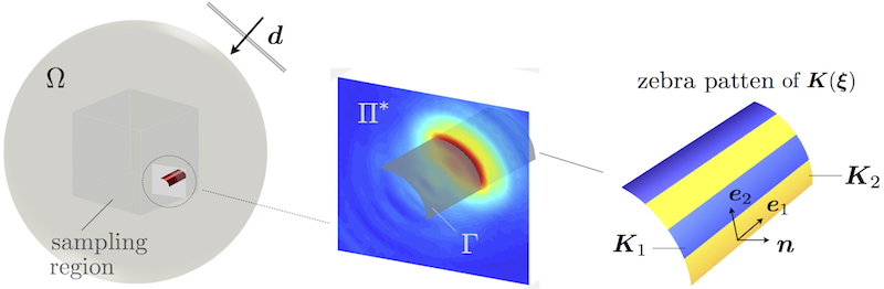
Testing configuration. The sensing setup, shown in Fig. 2, features a “true” cylindrical fracture of length and radius . The fracture is endowed with a piecewise-constant (“zebra”) distribution of interfacial stiffness on , alternating between and , where
in terms of the orthonormal basis shown in the figure. The shear modulus, mass density, and Poisson’s ratio of the background solid are taken as , and , whereby the shear and compressional wave speeds read and , respectively. The interaction of with incident (P- and S-) plane waves, propagating in direction , gives rise to the scattered wavefield solving (2) – whose far-field pattern is then computed on the basis of (21).
Far-field operator. For both illumination and sensing purposes, the unit sphere is sampled by a uniform grid of observation directions, specified by the polar () and azimuthal () angle values. With reference to (86), note that both the polarization vector of an incident plane wave and the far-field pattern of the scattered wave each have only three nontrivial components. In this setting, the discretized far-field operator F is represented as a matrix () with components
| (69) |
where
| (70) |
and are specified in (86). Unless stated otherwise, we assume and .
Noisy data. To account for the presence of noise in measurements, we consider the perturbed far-field operator
| (71) |
where is the identity matrix, and is the noise matrix of commensurate dimension whose components are uniformly-distributed (complex) random variables in . On the basis of definition (53), one has which in the sequel takes values of up to . With reference to Remark 3, the region of interest
Trial far-field pattern. With reference to Remark 3, the GLSM indicator map (67) is constructed by solving (55) for the minimizer of (54) over a grid of trial infinitesimal fractures , where denotes the sampling point and is a unitary rotation matrix. In what follows, this is accomplished by taking L to be a vanishing penny-shaped fracture with unit normal , i.e. by setting the FOD in (42) as . Writing for brevity , one in particular finds that
| (72) |
Recalling (86), one may note that for each observation direction , (72) has only three non-trivial components in the reference orthonormal basis, which are for consistency with (70) arranged as a vector
| (73) |
Accordingly, the far-field equation (41) takes the discretized form
| (74) |
thus forming the basis for computing GLSM and LSM indicator functionals.
7.1 Fracture indicators
As shown in Fig. 2, the search area i.e. the sampling region is a cube of side 2 where the featured (GLSM and LSM) indicator functionals are evaluated. The resulting distributions are plotted either in three dimensions, or in the mid-section of the “true” cylindrical fracture (see Fig. 2).
Sampling. In what follows, the search cube is probed by a uniform grid of sampling points , while the unit sphere – spanning possible fracture orientations – is sampled by a grid of trial normal directions . Accordingly, the fracture indicator map is constructed by solving (74) for a total of trial pairs .
GLSM indicator. With reference to (55) and (69)-(74), a discretized version of the GLSM solution vector, , is computed by solving the linear system
| (75) |
where is the Hermitian operator; is evaluated on the basis of definitions (45) and (46); and, following [3],
| (76) |
Here is a regularization parameter of the classical LSM solution (78), computed via the Morozov discrepancy principle [23]. With reference to (67), the GLSM indicator function is then obtained as
| (77) |
LSM indicator. To gain better insight into the effectiveness of the proposed approach, the GLSM reconstruction is compared to a corresponding LSM map. The latter is computed on the basis of a Tikhonov-regularized solution to (74), namely
| (78) |
where the regularization parameter is obtained by way of Morozov discrepancy principle [23]. On the basis of (78), the LSM indicator functional is constructed following [11] as
| (79) |
7.2 Results
In the sequel, the arclength () of a “true” cylindrical fracture in its mid-plane, see Fig. 2, is used as a reference length to gauge the illuminating shear wavelength .
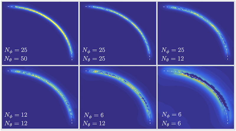
Density of the sensing grid. Taking , Fig. 3 illustrates the sensitivity of the GLSM indicator (77) to the spatial density of sensory data, given by incident/observation directions over the unit sphere. This is done by gradual downsampling of the default sensing grid. From the panels, it is apparent that for satisfactory geometric reconstruction, the sensing grid should carry at least 100 test directions over . In what follows, the (full-aperture) reconstructions are implemented using a grid.
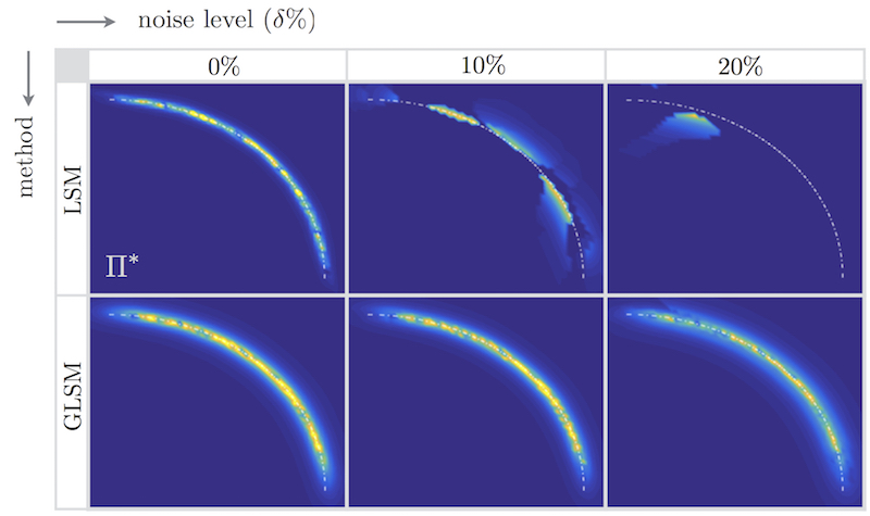
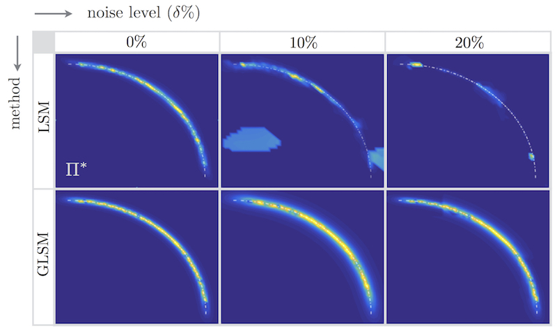
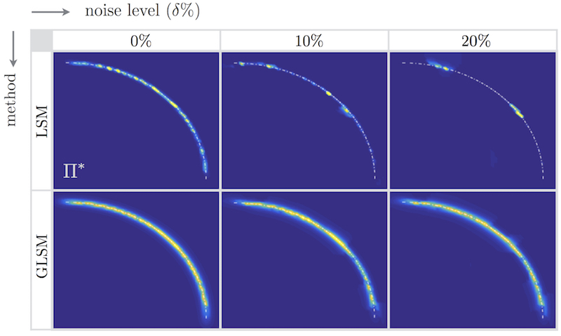
Sensitivity to measurement noise. Assuming full-aperture illumination and sensing, the GLSM and LSM indicators are next compared in terms of their robustness against noise in the far-field data. With reference to (71), the levels of “white” noise used to contaminate the boundary integral simulations of the forward scattering problem are taken . On focusing the comparison on the mid-section of a “true” fracture, the results are shown in Figs. 6, 6, and 6 assuming the illuminating wavelengths of , , and , respectively. Note that . As can be seen from the display, the GLSM indicator (77) inherits the superior localization ability of its LSM predecessor (79), while carrying far greater robustness to noise in the sensory data.
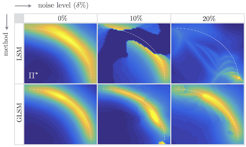
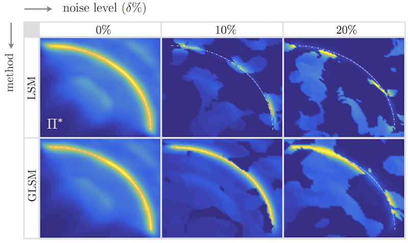
Effect of the sensing aperture. The ramifications of an incomplete aperture on the quality of fracture reconstruction are illustrated in Figs. 9 and 9, where only the “upper” half of in Fig. 2 is available for the purposes of illumination and observation. More specifically, Figs. 9 and 9 depict the GLSM and LSM fields in the mid-section of at “long” () and “short” () excitation wavelengths, respectively, constructed from the half-aperture sensory data. While the loss of resolution in both GLSM and LSM maps is clear relative to Figs. 6 and 6, it is noted that (for the problem under consideration) the GLSM indicator offers far better robustness to noise, providing acceptable reconstruction of for as high as .
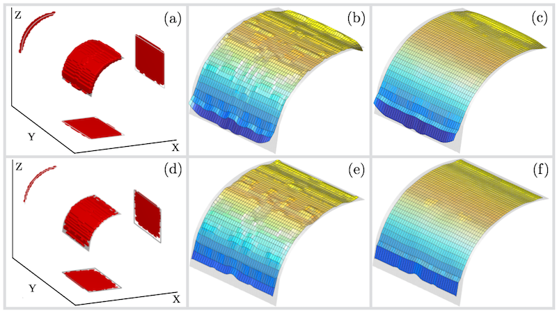
3D reconstruction. For completeness, Fig. 9 illustrates the full-aperture GLSM reconstruction of inside the sampling region , assuming and (top panels) and and (bottom panels). For clarity, the indicator maps are thresholded by , i.e. only the sampling points whose values are higher than ten percent of the global maximum value are shown (left panels). Then, a scattered interpolant is constructed based on thus obtained 3D cloud of points, giving an optimal reconstruction of the fracture surface. The latter is generated by (i) projecting the thresholded GLSM map onto a reference plane (the plane in this example), and (ii) defining a suitable grid of points covering the projected area. This forms the sought-for input for the scattered interpolant providing a 3D reconstruction of the fracture interface, as shown in the middle panels of Fig. 9. Due in part to a scattered nature of the interpolant, thus obtained fracture surface will suffer from some artificial roughness – that depends for example on the density of sampling points and an ad-hoc thresholding parameter. This issue may be mitigated by implementing a suitable spatial (e.g. moving average) filter, as shown in the right panels of Fig. 9.
8 Conclusions
The Generalized Linear Sampling Method (GLSM) combined with the -factorization technique form a fast, yet robust, platform for the geometric reconstruction of heterogeneous (and dissipative) discontinuity surfaces from scattered wavefield data. It is illustrated that the GLSM indicator possesses little sensitivity to (the reasonable levels of) measurement noise – that is comparable to the robustness of TS, while inheriting the top-tier localization property of the classical LSM, which guarantees a high-quality geometric characterization of the fracture – notwithstanding the frequency regime of excitation and the unknown (generally heterogeneous) interfacial stiffness . Such attributes carries a remarkable potential for developing a GLSM-based hybrid approach for not only geometric reconstruction of hidden fractures, but also identification of their interfacial condition (e.g. retrieval of in the present work) from scattered field data. Furthermore, this approach may be naturally and rigorously extended to other sensing configurations and to more sophisticated background-domain geometries. It should also be noted that the analysis in this study does not require the fracture surface to be connected, so one should be able to use the GLSM for simultaneous imaging of multiple fractures in the medium.
Appendix A Proof of equation (13)
Appendix B Elastodynamic fundamental stress tensor
Appendix C Proof of Lemma 4.1
Consider the orthonormal bases and , where and denote respectively the directions of observation and plane-wave incidence. On representing the far-field pattern (resp. the polarization vector ) in the (resp. ) basis, definition (23) of the far-field kernel can be written in matrix form as
| (86) |
In this setting, the reciprocity statement (25) can be rewritten as
| (87) |
This section aims to extend Lemma 1 in [15] to cater for the scattering problem (2)-(6) with its particular boundary condition, (4), at the fracture interface . With such result in place, the distilled reciprocity claim (87) follows immediately as a consequence of Theorem 1 and its corollaries in [15]. To this end, consider two distinct total fields
where satisfies (2)-(6) with . On adopting Twersky’s notation [34]
Lemma 1 in [15] states that , where is a ball of radius sufficiently large so that . By substituting the Navier equation
into Betti’s third formula [24] written for domain , one finds that
| (88) |
where, thanks to the jump condition on in (2) and contact law (4), one has
| (89) | ||||
Due to symmetry of , one has and consequently thanks to (88).
Appendix D Proof of Lemma 5.1
With reference to the Herglotz operator given by (26) and a fracture opening displacement (FOD) profile , consider the duality product
| (90) |
Thanks to (18) and the linearity of , the right-hand side of (90) can be recast as
On recalling that for arbitrary smooth surface
where is given by (3) and is the unit normal on , one finds that
As a result,
By virtue of (16) and (20) which verify , one finds that
which establishes (28).
Appendix E Proofs of Theorem 6.7 and Theorem 6.9
Proof of Theorem 5.7.
Consider the following:
-
•
Let . By definition, such that . Then, by recalling the continuity of (Lemma 5.6) and the range denseness of (Lemma 5.2), one may find for every such that . Now, let us observe that
-
i) by the continuity of (Lemma 6.5), one has
-
iii) thanks to the definitions of and , one has
As a result, it immediately follows that
(91) whereby which implies .
-
-
•
Next, let . Let us by contradiction assume that ; then, for some constant independent of , one has for an extracted subsequence of . The coercivity of then implies that is also bounded. As is reflexive, one may suppose that up to an extracted subsequence, weakly converges to some . In fact, since the latter set is convex. Now, since is compact, strongly converges to as . Recalling the definition of and the fact that as thanks to the range denseness of , one may observe that as . Thus, which is a contradiction. Accordingly, necessitates which in turn implies .
Proof of Theorem 5.9.
The logic of this proof follows that of Theorem 6.7, and entails the following steps.
- •
-
•
Let , and assume to the contrary that . Using the coercivity of and triangle inequality, one finds
whereby . Then, there exists a subsequence such that and is bounded independently from . In light of Lemma 6.8, one may design this subsequence such that as , and thus as . The compactness of and boundedness of imply that a subsequence of converges to some in . The uniqueness of this limit implies that , which is a contradiction.
References
- [1] J.D. Achenbach. Reciprocity in Elastodynamics. North-Holland, Amsterdam, 1984.
- [2] L. Audibert. Qualitative methods for heterogeneous media. PhD thesis, Ecole Doctorale Polytechnique, 2015.
- [3] L. Audibert and H. Haddar. A generalized formulation of the linear sampling method with exact characterization of targets in terms of farfield measurements. Inverse Problems, 30:035011, 2014.
- [4] G. I. Barenblatt. Scaling (Cambridge texts in applied mathematics). Cambridge University Press, Cambridge, UK, 2003.
- [5] C. Bellis and M. Bonnet. Qualitative identification of cracks using 3d transient elastodynamic topological derivative: formulation and fe implementation. Comput. methods Appl. Mech. Engrg, 253:89–105, 2013.
- [6] M Bonnet. Boundary integral equations methods for solids and fluids. Wiley, 1999.
- [7] M. Bonnet. Fast identification of cracks using higher-order topological sensitivity for 2-d potential problems. Eng. Anal. Bound. Elem., 35:223–235, 2011.
- [8] Y. Boukari and H. Haddar. The factorization method applied to cracks with impedance boundary conditions. Inverse Probl Imag, 7:1123–1138, 2013.
- [9] L Bourgeois and E Lun ville. On the use of the linear sampling method to identify cracks in elastic waveguides. Inverse Problems, 29(2):025017, 2013.
- [10] James H. Bramble and Joseph E. Pasciak. A note on the existence and uniqueness of solutions of frequency domain elastic wave problems: a priori estimates in . J. Math. Anal. Appl., 345(1):396–404, 2008.
- [11] F. Cakoni and D. Colton. The linear sampling method for cracks. Inverse Problems., 19:279–295, 2003.
- [12] F. Cakoni and D. Colton. A qualitative approach to inverse scattering theory. Springer, Berlin, 2008.
- [13] M. Chamaillard, N. Chaulet, and H. Haddar. Analysis of the factorization method for a general class of boundary conditions. J. Inverse Ill-posed Probl., 22:643 – 670, 2014.
- [14] D. Colton and R. Kress. Inverse acoustic and electromagnetic scattering teory. Springer, Berlin, 1992.
- [15] G. Dassios, K. Kiriaki, and D. Polyzos. On the scattering amplitudes for elastic waves. Z. Angew. Math. Phys., 38:856–873, 1987.
- [16] G. Dassios and Z. Rigou. Elastic herglotz functions. SIAM J Appl Math, 55:1345–1361, 1995.
- [17] X. Fang, M. C. Fehler, Z. Zhu, Y. Zheng, and D. R. Burns. Reservoir fracture characterization from seismic scattered waves. Geophys. J. Int., 196:481 – 492, 2014.
- [18] B. B. Guzina and M. Bonnet. Topological derivative for the inverse scattering of elastic waves. Quart. J. Mech. Appl. Math., 57:161–179, 2004.
- [19] F. B. Hassen, Y. Boukari, and H. Haddar. Application of the linear sampling method to identify cracks with impedance boundary conditions. Inverse Probl. Sci. Eng., 21:210 – 234, 2013.
- [20] Park W. K. Music-type imaging of small perfectly conducting cracks with an unknown frequency. J Phys Conf Ser, 633(1):012005, 2015.
- [21] A. Kirsch and N. Grinberg. The factorization methods for inverse problems. Oxford University Press, Oxford, 2008.
- [22] R. Kress. Inverse scattering from an open arc. Math. Methods Appl. Sci., 18:267–293, 1995.
- [23] R. Kress. Linear integral equation. Springer, Berlin, 1999.
- [24] V. D. Kupradze, T. G. Gegelia, M. O. Basheleishvili, and T. V. Burchuladze. Three-dimensional problems of the mathematical theory of elasticity and thermoelasticity. North-Holland Publishing, Netherlands, 1979.
- [25] P. A. Martin and G. Dassios. Karp s theorem in elastodynamic inverse scattering. Inverse Problems, 9:97–111, 1993.
- [26] W. McLean. Strongly Elliptic Systems and Boundary Integral Equations. Cambridge University Press, Cambridge, 2000.
- [27] S. Minato and R. Ghose. Inverse scattering solution for the spatially heterogeneous compliance of a single fracture. Geophys. J. Int., 195:1878–1891, 2013.
- [28] S. Minato and R. Ghose. Imaging and characterization of a subhorizontal non-welded interface from point source elastic scattering response. Geophys. J. Int., 197:1090–1095, 2014.
- [29] P. Monk. Finite Element Methods for Maxwell’s Equations. Clarendon Press, Oxford, 2003.
- [30] W-K. Park. Inverse scattering from two dimensional thin inclusions and cracks. PhD thesis, Ecole Polytechnique, 2009.
- [31] W-K. Park. Multi-frequency topological derivative for approximate shape acquisition of curve-like thin electromagnetic inhomogeneities. J. of Math. Analy. and Appl., 404:501–518, 2013.
- [32] W. K. Park. Multi-frequency subspace migration for imaging of perfectly conducting, arc-like cracks in full- and limited-view inverse scattering problems. J comp phys, 283:52 – 80, 2015.
- [33] F. Pourahmadian and B. B. Guzina. On the elastic-wave imaging and characterization of fractures with specific stiffness. int. J Solids Struct., 71:126–140, 2015.
- [34] V. Twersky. Multiple scattering by arbitrary configuration in three dimensions,. J. Math. Phys., 3:83, 1962.
- [35] S. Ueda, S. Biwa, K. Watanabe, R. Heuer, and C. Pecorari. On the stiffness of spring model for closed crack. Int. J. Eng. Sci., 44:874–888, 2006.
- [36] M. Willis, D. Burns, R. Rao, B. Minsley, M. Toksoz, and L. Vetri. Spatial orientation and distribution of reservoir fractures from scattered seismic energy. Geophysics, 71:O43 – O51, 2006.
- [37] Y. Zheng, X. Fang, M. C. Fehler, and D. R. Burns. Seismic characterization of fractured reservoirs by focusing gaussian beams. Geophysics, 78:A23 – A28, 2013.