Stabilising Model Predictive Control for Discrete-time Fractional-order Systems

Abstract

In this paper we propose a model predictive control scheme for constrained fractional-order discrete-time systems. We prove that all constraints are satisfied at all time instants and we prescribe conditions for the origin to be an asymptotically stable equilibrium point of the controlled system. We employ a finite-dimensional approximation of the original infinite-dimensional dynamics for which the approximation error can become arbitrarily small. We use the approximate dynamics to design a tube-based model predictive controller which steers the system state to a neighbourhood of the origin of controlled size. We finally derive stability conditions for the MPC-controlled system which are computationally tractable and account for the infinite dimensional nature of the fractional-order system and the state and input constraints. The proposed control methodology guarantees asymptotic stability of the discrete-time fractional order system, satisfaction of the prescribed constraints and recursive feasibility.

,

1 Introduction

1.1 Background and Motivation

Derivatives and integrals of non-integer order, often referred to as fractional, are natural extensions of the standard integer-order ones which enjoy certain favourable properties: they are linear operators, preserve analyticity, and have the semigroup property [26, 15]. Nonetheless, fractional derivatives are non-local operators, that is, unlike integer-order ones, they cannot be evaluated at a given point by mere knowledge of the function in a neighbourhood of this point and for that reason they are suitable for describing phenomena with infinite memory [26].

Fractional dynamics seems to be omnipresent in nature. Examples of fractional systems include, but are not limited to, semi-infinite transmission lines with losses [4], viscoelastic polymers [15], magnetic core coils [38], anomalous diffusion in semi-infinite bodies [14] and biomedical applications [21] for which Magin et al. provided a thorough review [20]. A good overview of the applications of fractional systems in physics is given in [15] and [42].

A shift towards fractional-order dynamics in the field of pharmacokinetics may be observed after the classical in-vitro-in-vivo correlations theory proved to have faced its limitations [18]. Non-linearities, anomalous diffusion, deep tissue trapping, diffusion across capillaries, synergistic and competitive action and other phenomena give rise to fractional-order pharmacokinetics [7]. In fact, Pereira derived fractional-order diffusion laws for media of fractal geometry [25]. Increasing attention has been drawn on modelling and control of such systems [8, 9, 41], especially in presence of state and input constraints.

Model predictive control (MPC) is an advanced, successful and well recognized control methodology and its adaptation to fractional systems is of particular interest. The current model predictive control framework for fractional-order systems has been developed in a series of papers where integer-order approximations are used to formulate the control problem [33, 32, 1, 5, 34]. CARIMA (controlled auto-regressive moving average) models are often used in predictive control formulations for the approximation of the fractional dynamics [33, 32, 34, 16]. The CARIMA-based approach has been used in various applications such as the heating control of a semi-infinite rod [29], the power regulation of a solid oxide fuel cell [5] and various applications in automotive technology [35]. The celebrated Oustaloup approximation has also been used in MPC settings [33]. It should, however, be noted that such approximations aim at capturing the system dynamics in a range of operating frequencies and, as a result, are not suitable for a rigorous analysis and design of controllers for constrained systems. Additionally, all of the aforementioned works provide examples of unconstrained systems; this shortcoming was in fact identified in the recent paper [16].

Nevertheless, this profusion of purportedly successful paradigms of MPC for fractional-order systems is not accompanied by a proper stability analysis especially when input and state constraints are present. A common denominator of all approaches in the literature is that they approximate the actual fractional dynamics by integer-order dynamics and design controllers for the approximate system using standard techniques. No stability and constraint satisfaction guarantees can be deduced for the original fractional-order system. Currently, one of the very few works on constrained control for fractional-order systems is due to Mesquine et al. where, however, only input constraints are taken into account for the design of a linear feedback controller [23].

Hitherto, two approaches can be found in the literature in regard to the stability analysis of discrete-time fractional systems. The first one considers the stability of a finite-dimensional linear time-invariant (LTI) system, known as practical stability, but fails to provide conditions for the actual fractional-order system to be (asymptotically) stable [3, 13]. This approach is tacitly pursued in many applied papers where stability is established only for a finite-dimensional approximation of the fractional-order system [33, 36]. On the other hand, fractional systems can be treated as infinite-dimensional systems for which various stability conditions can be derived (See for example [12, Thm. 2]), but conditions are difficult to verify in practice let alone to use for the design of model predictive — or other — controllers.

1.2 Contribution

In this paper we describe a stabilising MPC framework for fractional-order systems (of the Grünwald-Letnikov type) subject to state and input constraints. We discretise linear continuous-time fractional dynamics using the Grünwald-Letnikov scheme which leads to infinite-dimensional linear systems. Using a finite-dimensional approximation we arrive at a linear time-invariant system with an additive uncertainty term which casts the discrepancy with the infinite-dimensional system. We then introduce a tube-based MPC control scheme which is known to steer the state to a neighbourhood of the origin which can become arbitrarily small as the order of the approximation of the fractional-order system increases. In our analysis, we consider both state and input constraints which we show that are respected by the MPC-controlled system. We finally prove that under a certain contraction-type condition the origin is an asymptotically stable equilibrium point for the MPC-controlled fractional-order system (see Section 3.2). In this work we provide, for the first time, asymptotic stability conditions (Theorem 4) and we propose a control methodology which guarantees the satisfaction of the prescribed state and input constraints.

This paper builds up on [39] where the unmodelled part of the system dynamics was cast as a bounded additive uncertainty term and used existing MPC theory to drive the system’s state in a neighbourhood of the origin without, however, providing any (asymptotic) stability conditions for the origin.

1.3 Mathematical preliminaries

The following definitions and notation will be used throughout the rest of this paper. Let $\mathbb{N}$, $\mathbb{R}^{n}$, $\mathbb{R}_{+}$, $\mathbb{R}^{m\times n}$ denote the set of non-negative integers, the set of column real vectors of length $n$, the set of non-negative numbers and the set of $m$-by-$n$ real matrices respectively. For any nonnegative integers $k_{1}\leq k_{2}$ the finite set $\{k_{1},\ldots,k_{2}\}$ is denoted by $\mathbb{N}_{[k_{1},k_{2}]}$. Let $x$ be a sequence of real vectors of $\mathbb{R}^{n}$. The $k$-th vector of the sequence is denoted by $x_{k}$ and its $i$-th element is denoted by $x_{k,i}$. We denote by $\mathcal{B}_{\epsilon}^{n}=\{x\in\mathbb{R}^{n}:\|x\|<\epsilon\}$ the open ball of $\mathbb{R}^{n}$ with radius $\epsilon$ and we use the shorthand $\mathcal{B}^{n}=\mathcal{B}_{1}^{n}$. We define the point-to-set distance of a point $z\in X$ from $A$ as $\mathrm{dist}(z,A)=\inf_{a\in A}\|z-a\|$. The space of bounded real sequences is denoted by $\ell^{\infty}$. We define the space $\ell^{\infty}_{n}$ of all sequences of real $n$-vectors $z$ so that $(z_{k,i})_{k}\in\ell^{\infty}$ for $i\in\mathbb{N}_{[1,n]}$.

Let $\Gamma$ be a topological real vector space and $A,B\subseteq\Gamma$. For $\lambda\in\mathbb{R}$ we define the scalar product $\lambda C=\{\lambda c:c\in C\}$ and the Miknowski sum $A\oplus B=\{a+b:a\in A,b\in B\}$. The Minkowski sum of a finite family of sets $\{A_{i}\}_{i=1}^{k}$ will be denoted by $\bigoplus_{i=1}^{k}A_{i}$. The Minkowski sum of a sequence of sets $\{A_{i}\}_{i\in\mathbb{N}}$ is denoted by $\bigoplus_{i\in\mathbb{N}}A_{i}$ or $\bigoplus_{i=0}^{\infty}A_{i}$ and is defined as the Painlevé-Kuratowski limit of $\bigoplus_{i=1}^{k}A_{i}$ as $k{\to}\infty$ [31]. The Pontryagin difference between two sets $A,B\subseteq\Gamma$ is defined as $A\ominus B=\{a\in A:a+b\in A,\forall b\in B\}$. A set $C$ is called balanced if for every $x\in C$, $-x\in C$.

2 Fractional-order Systems

2.1 Discrete-time fractional-order systems

Let $x:\mathbb{R}\to\mathbb{R}^{n}$ be a uniformly bounded function, i.e., there is a $M>0$ so that $\|x(t)\|\leq M$ for all $t\in\mathbb{R}$. The Grünwald-Letnikov fractional-order difference of $x$ of order $\alpha>0$ and step size $h>0$ at $t$ is defined as the linear operator [24, 30] $\Delta^{\alpha}_{h}:\ell_{n}^{\infty}\to\ell_{n}^{\infty}$:

$$\Delta^{\alpha}_{h}x(t)=\sum_{j=0}^{\infty}(-1)^{j}{\alpha\choose j}x(t-jh),$$ (1)

where ${\alpha\choose 0}=1$ and for $j\in\mathbb{N}$, $j>0$

$${\alpha\choose j}=\prod_{i=0}^{j-1}\frac{\alpha-i}{i+1}=\frac{\Gamma(\alpha+1)}{\Gamma(\alpha-j+1)j!}.$$ (2)

The forward-shifted counterpart of $\Delta^{\alpha}_{h}$ is defined as ${{}_{F}\Delta^{\alpha}_{h}}x(t)=\Delta^{\alpha}_{h}x(t+h)$. Now, define

$$c^{\alpha}_{j}=(-1)^{j}{\alpha\choose j}={j-\alpha-1\choose j},$$ (3)

and notice for all $j\in\mathbb{N}$ that $|c^{\alpha}_{j}|\leq\alpha^{j}/j!$, thus, the sequence $(c^{\alpha}_{j})_{j}$ is absolutely summable and, because of the uniform boundedness of $x$, the series in (1) converges, therefore, $\Delta^{\alpha}_{h}$ is well-defined. It is worth noticing that for $\alpha\in\mathbb{N}$ it is $c_{j}^{\alpha}=0$ for $j\geq\lceil\alpha\rceil$, but this property does not hold for $\alpha\notin\mathbb{N}$. As a result, at time $t$ and for non-integer orders $\alpha$ the whole history of $x$ is needed in order to estimate $\Delta^{\alpha}_{h}x(t)$.

The Grünwald-Letnikov difference operator gives rise to the Grünwald-Letnikov derivative of order $\alpha$ which is defined as [37, Sec. 20]

$$D^{\alpha}x(t)=\lim_{h\to 0^{+}}\frac{{}_{F}\Delta^{\alpha}_{h}x(t)}{h^{\alpha}}=\lim_{h\to 0^{+}}\frac{\Delta^{\alpha}_{h}x(t)}{h^{\alpha}},$$ (4)

insofar as both limits exist. This derivative is then used to describe fractional-order dynamical systems with state $x:\mathbb{R}\to\mathbb{R}^{n}$ and input $u:\mathbb{R}\to\mathbb{R}^{m}$ as follows:

$$\sum_{i=1}^{l}A_{i}D^{\alpha_{i}}x(t)=\sum_{i=1}^{r}B_{i}D^{\beta_{i}}u(t),$$ (5)

where $l,r\in\mathbb{N}$, $A_{i}$ are $B_{i}$ are matrices of opportune dimensions, all $\alpha_{i}$ and $\beta_{i}$ are nonnegative, and by convention $D^{0}x(t)=x(t)$ for any $x$.

In an Euler discretisation fashion we approximate the $D^{\alpha}$ in (5) using either $h^{-\alpha}{{}_{F}}\Delta^{\alpha}_{h}$ or $h^{-\alpha}\Delta^{\alpha}_{h}$ for a fixed step size $h$ as in [24]. In particular, we use ${{}_{F}}\Delta^{\alpha}_{h}$ for the derivatives of the state and $\Delta^{\alpha}_{h}$ for the input variables. We define $x_{k}=x(kh)$ and $u_{k}=u(kh)$ for $k\in\mathbb{Z}$ so the discretisation of (5) becomes

$$\sum_{i=1}^{l}\bar{A}_{i}\Delta_{h}^{\alpha_{i}}x_{k+1}=\sum_{i=1}^{r}\bar{B}_{i}\Delta_{h}^{\beta_{i}}u_{k},$$ (6)

with $\bar{A}_{i}=h^{-\alpha_{i}}A_{i}$ and $\bar{B}_{i}=h^{-\beta_{i}}B_{i}$. The involvement of infinite-dimensional operators in the system dynamics deem these systems computationally intractable and call for approximation methods for their simulation and the design of feedback controllers.

In what follows, we will approximate (6) by a finite-dimensional state-space system treating the approximation as a bounded additive disturbance. We then propose a control setting which guarantees robust stability properties for (6).

2.2 Finite-dimension approximation

Discrete-time fractional-order dynamical systems are essentially systems with infinite memory and an infinite number of state variables. As a result, standard stability theorems and control design methodologies for finite-dimensional systems cannot be applied directly. To this end we introduce the following truncated Grünwald-Letnikov difference operator of length $\nu$ given by

$$\Delta^{\alpha}_{h,\nu}x_{k}=\sum_{j=0}^{\nu}c_{j}^{\alpha}x_{k-j},$$ (7)

System (6) is the approximated by the following system using $\nu\geq 1$

$${\sum_{i=1}^{l}\bar{A}_{i}\Delta_{h,\nu}^{\alpha_{i}}x_{k+1}=\sum_{i=1}^{r}\bar{B}_{i}\Delta_{h,\nu}^{\beta_{i}}u_{k}}.$$ (8)

System (8) can be written in state space format as a linear time-invariant system with a proper choice of state variables $\tilde{x}_{k}$ as we shall explain in this section. In the common case where the right-hand side of (8) is of the simple form $Bu_{k}$, it is straightforward to recast the system in state-space form. Here, we study the more general case of equation (8), which can be written in the form

$$\sum_{j=0}^{\nu}\hat{A}_{j}x_{k-j+1}=\sum_{j=0}^{\nu}\hat{B}_{j}u_{k-j},$$ (9)

with $\hat{A}_{j}=\sum_{i=1}^{l}\bar{A}_{i}c_{j}^{\alpha_{i}}$ and $\hat{B}_{j}=\sum_{i=1}^{r}\bar{B}_{i}c_{j}^{\beta_{i}}$ for $j\in\mathbb{N}_{[0,\nu]}$. We hereafter assume that matrix $\hat{A}_{0}$ is nonsingular. With this assumption, the discrete-time dynamical system (9) becomes a normal system, that is, future states can be determined using past states in a unique fashion and can be written as a linear time-invariant system [10, Chap. 1]. Defining $\tilde{A}_{j}=-\hat{A}_{0}^{-1}\hat{A}_{j}$ and $\tilde{B}_{j}=\hat{A}_{0}^{-1}\hat{B}_{j}$, the dynamic equation (9) becomes

$$x_{k+1}=\sum_{j=0}^{\nu-1}\tilde{A}_{j}x_{k-j}+\sum_{j=1}^{\nu}\tilde{B}_{j}u_{k-j}+\tilde{B}_{0}u_{k}.$$ (10)

This can be written in state space form with state variable $\tilde{x}_{k}=(x_{k},x_{k-1},\ldots,x_{k-\nu+1},u_{k-1},\ldots,u_{k-\nu})^{\prime}$ as

$$\tilde{x}_{k+1}=A\tilde{x}_{k}+Bu_{k}.$$ (11)

System (11) is an ordinary finite-dimensional LTI system which will be used in the next section to formulate a model predictive control problem. Throughout the rest of the paper we assume that the pair $(A,B)$ is stabilisable.

The truncated difference operator $\Delta_{h,\nu}^{\alpha}$ introduces some error in the system dynamics. In particular, the fractional-order difference operator ${\Delta_{h}^{\alpha}}$ can be written as

$${\Delta_{h}^{\alpha}}=\Delta_{h,\nu}^{\alpha}+R^{\alpha}_{h,\nu},$$ (12)

where $R^{\alpha}_{h,\nu}:\ell^{\infty}_{n}\to\ell^{\infty}_{n}$ is the operator $R^{\alpha}_{h,\nu}(x_{k})=\sum_{j=\nu+1}^{\infty}c_{j}^{\alpha}x_{k-j}$. Let $X$ be a compact convex subset in $\mathbb{R}^{n}$ containing $0$ in its interior and at time $k$ assume that $x_{k-j}\in X$ for all $j\in\mathbb{N}$. Then, by the assumption that $x_{k-j}\in X$ for all $j\in\mathbb{N}$,

$$R^{\alpha}_{h,\nu}(x_{k})\in\bigoplus_{j=\nu+1}^{\infty}c_{j}^{\alpha}X.$$ (13)

For all $\nu\in\mathbb{N}$, the right-hand side of (13) is a convex compact set with the origin in its interior. Equation (6) can now be rewritten using the augmented state variable $\tilde{x}$ (cf. (11)) leading to the following linear uncertain system

$$\tilde{x}_{k+1}=A\tilde{x}_{k}+Bu_{k}+Gd_{k},$$ (14)

where $d_{k}$ is a (bounded) additive disturbance term (which depends on $x_{k-\nu-j}$ and $u_{k-\nu-j}$ for $j\in\mathbb{N}$) with $G=\left[\begin{smallmatrix}I&0&\ldots&0\end{smallmatrix}\right]^{\prime}$. Assume that $u_{k-j}\in U$ for $j=1,2,\ldots$ and $x_{k-j}\in X$ for $j\in\mathbb{N}$, where $X$ and $U$ are convex compact sets containing $0$ in their interiors. Then, $d_{k}$ is bounded in a compact set $D_{\nu}$ given by

$$D_{\nu}{=}D_{\nu}^{x}\oplus D_{\nu}^{u},$$ (15)

where

$$D_{\nu}^{x} =\bigoplus_{i=1}^{l}-\hat{A}_{0}^{-1}\bar{A}_{i}\bigoplus_{j=\nu+1}^{\infty}c_{j}^{\alpha_{i}}X,$$ (16a)

$$D_{\nu}^{u} =\bigoplus_{i=1}^{r}\hat{A}_{0}^{-1}\bar{B}_{i}\bigoplus_{j=\nu+1}^{\infty}c_{j}^{\beta_{i}}U.$$ (16b)

Under the prescribed assumptions $D_{\nu}$ is a compact set. Hereafter, we shall use the notation $A^{\ast}_{i}=-\hat{A}_{0}^{-1}\bar{A}_{i}$ and $B^{\ast}_{i}=\hat{A}_{0}^{-1}\bar{B}_{i}$.

Recall that for a balanced set $C\subseteq\mathbb{R}^{n}$ and scalars $\lambda_{1},\lambda_{2}$ it is $\lambda_{1}C\oplus\lambda_{2}C=(|\lambda_{1}|+|\lambda_{2}|)C$. In case $X$ and $U$ are balanced sets, the above expressions for $D_{\nu}^{x}$ and $D_{\nu}^{u}$ can be simplified. First, for $\nu\in\mathbb{N}$, we define the function $\Psi_{\nu}:\mathbb{R}_{+}\to\mathbb{R}_{+}$ as follows

$$\Psi_{\nu}(\alpha)=\sum_{j=\nu+1}^{\infty}|c_{j}^{\alpha}|.$$ (17)

Then, $D_{\nu}^{x}$ is written as the finite Minkowski sum

$$D_{\nu}^{x}=\bigoplus_{i\in\mathbb{N}_{[1,l]}}A^{\ast}_{i}\Psi_{\nu}(\alpha_{i})X,$$ (18)

and of course the same simplification applies to $D_{\nu}^{u}$ if $U$ is a balanced set. Notice that the computation of $D_{\nu}^{x}$ by (18) boils down to determining a finite Minkowski sum, which is possible when constraints are polytopic [11], while overapproximations exists when they are ellipsoidal [17].

The size of $D_{\nu}$ is controlled by the choice of $\nu$; $D_{\nu}$ can become arbitrarily small provided that a sufficiently large $\nu$ is chosen. Notice also that $D_{\nu}\to\{0\}$ as $\nu\to\infty$. In light of (14), the fractional system can be controlled by standard methods of robust control such as min-max [6] or tube-based MPC [28]; here we use the latter approach. In what follows, we elaborate on how the tube-based MPC methodology can be applied for the control of fractional-order systems.

Various integer-order approximation methodologies have been proposed in the literature such as continued fraction expansions of the system’s transfer function, the approximation methods of Carlson, Matsuda, Oustaloup, Chareff and more (see [43] for an overview). Methods which are based on the approximation of the system dynamics in a given frequency range cannot lead to the formulation of an LTI system with a bounded disturbance as in (14) and, as a result, cannot be used to guarantee stability for constrained systems as we will present in the next section.

3 Model Predictive Control

3.1 Tube-based Model Predictive Control

Model predictive control is a class of advanced control algorithms where the control action is calculated at every time instant by solving a constrained optimisation problem where a performance index is optimised. This performance index is used to choose an optimal sequence of control actions among the set of such admissible sequences, while corresponding state sequences are produced using a system model. The first element of the optimal sequence is applied to the system; this control scheme defines the receding horizon control approach [28]. When the process model is inaccurate, the modelling error must be taken into account to guarantee the satisfaction of state constraints and closed-loop stability properties. Tube-based MPC is a flavour of MPC which leads to robust closed-loop stability while the accompanying optimisation problem is computationally tractable (unlike the min-max version of MPC [28]).

Here, we require that the state and input variables are constrained in the sets $X\subseteq\mathbb{R}^{n}$ and $U\subseteq\mathbb{R}^{m}$ respectively, both convex, compact and contain the origin in their interior. The constraints are written as follows, this time involving $\tilde{x}$:

$$\tilde{x}_{k} \in\tilde{X},$$ (19a)

$$u_{k} \in U,$$ (19b)

for all $k\in\mathbb{N}$ and where $\tilde{X}=X^{\nu}\times U^{\nu}$, i.e., $\tilde{x}=(x_{k},x_{k-1},\ldots,x_{k-\nu+1},u_{k-1},\ldots,u_{k-\nu})^{\prime}\in\tilde{X}$ if and only if $x_{k-i}\in X$ for $i\in\mathbb{N}_{[0,\nu-1]}$ and $u_{k-i}\in U$ for all $i\in\mathbb{N}_{[1,\nu]}$. Typically, in MPC $\tilde{X}$ and $U$ can be polytopes or ellipsoids, but for our analysis no particular assumptions on $X$ and $U$ need to be imposed.

The fractional-order system is controlled by an input $u$ which is computed according to

$$u_{k}=v_{k}+Ke_{k},$$ (20)

where $v_{k}$ is a control action computed by the tube-based MPC controller and $e_{k}$ is defined as the deviation between the actual system state and the response of the nominal system, that is $e_{k}=\tilde{x}_{k}-\tilde{z}_{k}$. In particular, the nominal dynamics in terms of the nominal state $\tilde{z}_{k}$ with input $v_{k}$ is

$$\tilde{z}_{k}=A\tilde{z}_{k-1}+Bv_{k-1}.$$ (21)

Matrix $K$ in (20) is chosen so that the matrix $A_{K}=A+BK$ is strongly stable. For $k\in\mathbb{N}$ let

$$S_{k}^{\nu}=\bigoplus_{i=0}^{k}A_{K}^{i}GD_{\nu}.$$ (22)

The set $S_{\infty}^{\nu}=\lim_{k\to\infty}S_{k}^{\nu}$, is well-defined (the limit exists), is compact, and is positive invariant for the deviation dynamics $e_{k+1}=A_{K}e_{k}+Gd_{k}$. In what follows, $S_{\infty}^{\nu}$ will be assumed to contain the origin in its interior. For the needs of tube-based MPC, any over-approximation of $S_{\infty}^{\nu}$ may be used instead [27].

Having chosen $\tilde{z}_{0}=\tilde{x}_{0}$, it is $\tilde{x}_{k}\in\{\tilde{z}_{k}\}\oplus S_{\infty}^{\nu}$ for all $k\in\mathbb{N}$. This implies that constraint (19a) is satisfied if $\tilde{z}_{k}\in X\ominus S_{\infty}^{\nu}$ and constraint (19b) is satisfied if $v_{k}\in U\ominus KS_{\infty}^{\nu}$. These constraints will then be involved in the formulation of the MPC problem which produces the control actions $v_{k}=v_{k}(\tilde{z}_{k})$.

The MPC problem amounts to the minimisation of a performance index $V_{N}$ along an horizon of future time instants, known as the prediction horizon, given the state of the nominal system $\tilde{z}_{k}$ at time $k$. Let $N$ be the prediction horizon. We use the notation $\tilde{z}_{k+i\mid k}$ for the predicted state of the nominal system at time $k+i$ using feedback information at time $k$. Let $\mathbf{v}_{k}=\{v_{k+i\mid k}\}_{i\in\mathbb{N}_{[0,N-1]}}$ be a sequence of input values and $\{\tilde{z}_{k+i\mid k}\}_{i\in\mathbb{N}_{[1,N]}}$ the corresponding predicted states obtained by (21), i.e., it is

$$\tilde{z}_{k+i+1\mid k}=A\tilde{z}_{k+i\mid k}+Bv_{k+i\mid k},\text{ for }i\in\mathbb{N}_{[0,N-1]}$$ (23)

We introduce a performance index $V_{N}:\mathbb{R}^{\bar{n}}{\times}\mathbb{R}^{mN}{\to}\mathbb{R}_{+}$ given the current state of the system $\tilde{z}_{k\mid k}=\tilde{z}_{k}$

$$V_{N}(\tilde{z}_{k\mid k},\mathbf{v}_{k}){=}V_{f}(\tilde{z}_{k+N\mid k}){+}\sum_{i=0}^{N-1}\ell(\tilde{z}_{k+i\mid k},v_{k+i\mid k}),$$ (24)

where $\ell$ and $V_{f}$ are typically quadratic functions. We assume that $\ell(z,v)=z^{\prime}Qz+v^{\prime}Rv$, where $Q$ is symmetric, positive semidefinite and $R$ is symmetric positive definite and $V_{f}(z)=z^{\prime}Pz$, where $P$ is symmetric and positive definite. The following constrained optimisation problem is then solved:

$$\mathbb{P}_{N}{:}\ V_{N}^{\star}(\tilde{z}_{k})=\min_{\mathbf{v}_{k}\in\mathcal{V}_{N}(\tilde{z}_{k})}V_{N}(\tilde{z}_{k},\mathbf{v}_{k}),$$ (25)

where $\mathcal{V}_{N}(\tilde{z}_{k})$ is the set of all input sequences $\mathbf{v}_{k}$ with $v_{k+i\mid k}\in U\ominus KS$ for all $i{\in}\mathbb{N}_{[0,N-1]}$ so that $\tilde{z}_{k+i\mid k}\in\tilde{X}\ominus S$, for all $i{\in}\mathbb{N}_{[0,N{-}1]}$ and $\tilde{z}_{k+N\mid k}\in\tilde{X}_{f}$ given that $\tilde{z}_{k\mid k}=\tilde{z}_{k}$, where $S$ is any over-approximation of $S_{\infty}^{\nu}$, i.e., $S\supseteq S_{\infty}^{\nu}$ and $\tilde{X}_{f}\subseteq\tilde{X}$ is the terminal constraints set. In what follows we always assume that $\tilde{X}\ominus S$ and $U\ominus KS$ are nonempty sets with the origin in their interior. In regard to the terminal cost function $V_{f}$ and the terminal constraints set $\tilde{X}_{f}$ we assume the following:

Assumption 1.

$V_{f}$ and $\tilde{X}_{f}$ satisfy the standard stabilising conditions in [22] which are (i) $\tilde{X}_{f}\subseteq\tilde{X},$ $0\in\tilde{X}_{f}$, $\tilde{X}_{f}$ is closed, (ii) there is a controller $\kappa_{f}:\tilde{X}_{f}\to U$ so that $\tilde{X}_{k}$ is positively invariant for the nominal system (21) under $\kappa_{f}$, i.e., $A\tilde{x}+B\kappa_{f}(\tilde{x})\in\tilde{X}_{f}$ for all $\tilde{x}\in\tilde{X}_{f}$, and (iii) $V_{f}$ is a local Lyapunov function in $\tilde{X}_{f}$ for the $\kappa_{f}$-controlled system.

Remark 2.

Matrix $P$ in $V_{f}$ is typically chosen to be the (unique) solution of the discrete-time algebraic Riccatti equation $P=(A+BF)^{\prime}P(A+BF)+Q+F^{\prime}RF$ with $F=-(B^{\prime}PB+R)^{-1}B^{\prime}PA$ and $\tilde{X}_{f}$ to the maximal invariant constraint admissible set for the system $\tilde{z}_{k+1}=(A+BF)\tilde{z}_{k}$. Alternatively, one may choose $\tilde{X}_{f}$ to be an ellipsoid of the form $\tilde{X}_{f}=\{z:V_{f}(z)\leq\gamma\}$ and $\gamma>0$ is chosen so that $\tilde{X}_{f}\subseteq\tilde{X}$ and $K\tilde{X}_{f}\subseteq U$; such a set can be computed according to [2, Sec. 8.4.2]. The latter is a better choice from a computational point of view especially in high dimensional spaces although the optimisation problem becomes a quadratically-constrained quadratic problem.   $\diamond$

The solution of $\mathbb{P}_{N}$, namely the optimiser

$$v^{\star}(\tilde{z}_{k})=\operatorname*{argmin}\limits_{\mathbf{v}_{k}\in\mathcal{V}_{N}(\tilde{z}_{k})}V_{N}(\tilde{z}_{k},\mathbf{v}_{k}),$$ (26)

defines the control law $\kappa_{N}(\tilde{z}_{k})=v_{0}^{\star}(\tilde{z}_{k})$ and leads to the closed-loop dynamics

$$\tilde{x}_{k+1} =A\tilde{x}_{k}+B\rho(\tilde{z}_{k},\tilde{x}_{k})+Gd_{k},$$ (27a)

$$\tilde{z}_{k+1} =A\tilde{z}_{k}+B\kappa_{N}(\tilde{z}_{k}).$$ (27b)

Stability properties of the closed-loop system are hereafter derived and stated with respect to the composite system (27) with state variable $(\tilde{x},\tilde{z})$.

3.2 Stabilising conditions

In this section we study the stability properties of the controlled closed-loop system presented previously. Apart from the well-known stability results in robust MPC, we prove that, under certain conditions, the controlled trajectories of the system are asymptotically stable to the origin (see Theorem 4).

The following result, which readily follows from [28, Prop. 3.15], states that the system’s state converges towards $S_{\infty}$ exponentially provided that $S=S_{\infty}$ is used in the formulation of the MPC problem.

Theorem 3 (Rawlings & Mayne [28]).

Assume that the MPC control law $\kappa_{N}$ stabilises the nominal dynamical system (27b). The set $S_{\infty}\times\{0\}$ is exponentially stable for system (27) with region of attraction $(Z_{N}\oplus S_{\infty})\times Z_{N}$, where $Z_{N}$ is the domain of $\mathcal{V}_{N}$, i.e., $Z_{N}=\{x:\mathcal{V}_{N}(x)\neq\varnothing\}$.

In addition, the controlled trajectory of the system’s state $x_{k}$ and input $u_{k}$ satisfy constraints (19) at all time instants $k\in\mathbb{N}$.

Notice that $S_{\infty}$ can become arbitrarily small with an appropriate choice of $\nu$ and the system’s state can be steered this way very close to the origin, although, in practice large values of $\nu$ should be avoided to limit the computation complexity of optimisation problem $\mathbb{P}_{N}$. In addition to Theorem 3, we are going to prove that the state converges exactly to the origin and the origin is an asymptotically stable equilibrium point of the controlled system under certain conditions. The stability conditions we are about to postulate are easy to verify and can be used for the design of stabilising model predictive controllers. Hereafter, we shall assume that there are no derivatives acting on system’s inputs, i.e., $r=1$, $\beta_{1}=0$. The main result of this section is stated as follows:

Theorem 4 (Asymptotic stability).

Assume that $X$ is compact and balanced, Assumption 1 is satisfied and there is an $\epsilon\in(0,1)$ so that the following condition holds:

$$\bigoplus_{j\in\mathbb{N}}A_{K}^{j}GD \subseteq\mathcal{B}_{\epsilon}^{\bar{n}},$$ (28)

where $D$ is the set

$$D=\bigoplus_{i{\in}\mathbb{N}_{[1,l]}}\Psi_{\nu}(\alpha_{i})A^{\ast}_{i}\mathcal{B}^{n}.$$ (29)

Assume also that there is a $\sigma>0$ so that $S_{\infty}\subseteq\mathcal{B}_{\sigma}^{\bar{n}}\subseteq Z_{N}\oplus S_{\infty}$. Then, the origin is an asymptotically stable equilibrium point for (27).

The proof can be found in the appendix.

Remark 5.

The vector space $\mathbb{R}^{\bar{n}}$ can be written as the direct sum of vector spaces $L_{1},\ldots,L_{\nu}$, each of dimension $n$, so that $\tilde{x}_{k}\in\mathbb{R}^{\bar{n}}$ if and only if $x_{k-j+1}\in L_{j}$ for $j\in\mathbb{N}_{[1,\nu]}$. Assume that $S_{\infty}\cap L_{i}$ has nonempty interior in the topology of $L_{i}$. Then, in Theorem 4 one may drop the requirement that $S_{\infty}\subseteq\mathcal{B}_{\sigma}^{\bar{n}}$ by replacing the norm $\|\cdot\|$ of $\mathbb{R}^{\bar{n}}$ by the Minkowski functional of $S_{\infty}$, that is

$$\mathrm{p}[S_{\infty}](\tilde{x})=\inf_{\lambda>0}\{\lambda S_{\infty}\ni\tilde{x}\}.$$ (30)

The norm-ball $\mathcal{B}_{\epsilon}^{\bar{n}}$ becomes $\mathcal{B}_{\epsilon}^{\bar{n}}=\{x:\mathrm{p}[S_{\infty}](x)<\epsilon\}$ and the induced matrix norm is modified accordingly, while on $L_{i}$ we replace the norm by $\mathrm{p}[S_{\infty}\cap L_{i}](x)$. This is based on a useful property of $\mathrm{p}[S_{\infty}\cap L_{i}](x)$ which is stated in Appendix B.  $\diamond$

Remark 6.

Assume that $D$ in Theorem 4 is a polytope (for example, the 1-norm or the infinity-norm is used). Using the results presented in [27], given a tolerance $t>0$, there is a $\beta>1$ and an $s\in\mathbb{N}$ so that the polytope

$$F_{\beta,s}=\beta\bigoplus_{i=0}^{s}A_{K}^{i}GD$$

be an $t$-outer approximation of

$$F=\bigoplus_{i=0}^{\infty}A_{K}^{i}GD,$$ (31)

in the sense that $F\subseteq F_{\beta,s}\subseteq F\oplus\mathcal{B}_{t}^{\bar{n}}$. Then, the stabilising condition of Theorem 4 is satisfied if $F_{\beta,s}\subseteq\mathcal{B}_{\epsilon}^{\bar{n}}$ and this condition is easier to check computationally.  $\diamond$

Remark 7.

Since $A_{K}$ is a strictly Hurwitz matrix, there is a finite $a\in\mathbb{N}$ so that $\|A_{K}^{j}\|<1$ for all $j>a$. Then $F$ can be written as

$$F=\bigoplus_{i=0}^{a}A_{K}^{i}GD\oplus\bigoplus_{i=0}^{\infty}A_{K}^{a+1+i}GD,$$ (32)

where the first term is finitely determined and in case $D$ is a polytope, it is also a polytope. Let $\delta^{\ast}=\max_{d\in D}\|d\|$ (which is well-defined and finite because $D$ is compact). The second term of $F$ in (32) can be over-approximated

$$\bigoplus_{i=0}^{\infty}A_{K}^{a+1+i}GD \subseteq\bigoplus_{i=0}^{\infty}A_{K}^{a+1+i}G\mathcal{B}_{\delta^{\ast}}\subseteq\bigoplus_{i=0}^{\infty}\mathcal{B}_{\delta^{\ast}\|A_{K}^{a+1}\|^{i}}$$

$$\subseteq\mathcal{B}_{\delta^{\ast}\sum_{i=0}^{\infty}\|A_{K}^{a+1}\|^{i}}=\mathcal{B}_{\frac{\delta^{\ast}}{1-\|A_{K}^{a+1}\|}}.$$

This is based on the observation that for a matrix $B\in\mathbb{R}^{n\times m}$ it is $B\mathcal{B}^{m}\subseteq\mathcal{B}_{\|B\|}^{n}$, where $\|B\|$ is the operator norm defined in Section 1.3. As a result we have that for $B_{1},B_{2}\in\mathbb{R}^{n\times m}$, it is $B_{1}\mathcal{B}^{m}\oplus B_{2}\mathcal{B}^{m}\subseteq\mathcal{B}^{n}_{\|B_{1}\|}\oplus\mathcal{B}^{n}_{\|B_{2}\|}\subseteq\mathcal{B}^{n}_{\|B_{1}\|+\|B_{2}\|}$. If $a$ is adequately large and/or $\delta^{\ast}$ is adequately small, it will be $\frac{\delta^{\ast}}{1-\|A_{K}^{a+1}\|}<\epsilon<1$ (for some $\epsilon$) and then we can check the following stability condition

$$\bigoplus_{i=0}^{a}A_{K}^{i}GD\subseteq\mathcal{B}_{\epsilon-\frac{\delta^{\ast}}{1-\|A_{K}^{a+1}\|}},$$ (33)

which entails stabilising condition (28) and is easier to verify.  $\diamond$

3.3 Computational complexity

In this section we discuss the computational complexity of the proposed scheme and give some guidelines for the selection of $\nu$. By Theorem 4, an adequately large value of $\nu$ leads to the satisfaction of the stabilising conditions of the theorem. Naturally, for a given $\alpha>0$, one would be interested to know the minimum order of approximation $\nu_{\epsilon}^{\alpha}$ for which $\Psi_{\nu_{\epsilon}^{\alpha}}(\alpha)<\epsilon$, where $\epsilon>0$ is a desired threshold.

With $\nu=\nu_{\epsilon}^{\alpha}$, the MPC problem one needs to solve is formulated for a system that has $\nu_{\epsilon}^{\alpha}$ as many states as the original fractional system. Clearly, a parsimonious selection of $\nu$ is of major importance for a computationally tractable controller design. The designer needs to choose $\epsilon$ in order to strike a good balance between performance and computational cost. Indicatively, for $\epsilon=0.05$ and $\alpha=0.7$ we need $\nu=15$, whereas for the same $\epsilon$ and $\alpha=1.3$ we need $\nu=4$.

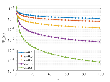
Figure 1: Dependence of $\Psi_{\nu}(\alpha)$ on $\nu$ for various values of $\alpha$. The smaller $\alpha$ is, the slower the convergence of $\Psi_{\nu}(\alpha)$ becomes.

4 Numerical Example

We apply the proposed methodology to the fractional-order system $D^{\alpha}x(t)=Ax(t)+Bu(t)$ with

$$A=\begin{bmatrix}1&0.9\\ -0.9&-0.2\end{bmatrix},B=\begin{bmatrix}0\\ 1\end{bmatrix},$$ (34)

and $x\in\mathbb{R}^{2}$, $u\in\mathbb{R}$ and $\alpha=0.7$. Matrix $A$ has eigenvalues $0.4\pm 0.678i$ and the unactuated open-loop system is unstable. We discretise the system with sampling period $h=0.1$ and we use $\nu=20$ based on Figure 1 so that $\Psi_{\nu}(\alpha)\cong 0.041$ is adequately small (leading to an adequately small set $D_{\nu}$). This way, we derive a discrete-time LTI system of the form $\tilde{x}_{k}=A\tilde{x}_{k-1}+Bu_{k-1}$ as in Section 2.2. The system state and input are subject to the constraints

$$-\begin{bmatrix}3\\ 3\end{bmatrix}\leq x_{k}\leq\begin{bmatrix}3\\ 3\end{bmatrix},$$ (35a)

$$-0.5\leq u_{k}\leq 0.5.$$ (35b)

The terminal cost $V_{f}$ and the terminal constraints set $\tilde{X}_{f}$ were computed according so that Assumption 1 is satisfied. In particular $\tilde{X}_{f}$ was chosen to be a sublevel set of $V_{f}$ as explained in Remark 2, that is $X_{f}=\{x:V_{f}(x)\leq\gamma\}$, where $\gamma=0.015$. The prediction horizon was chosen to be $N=100$ and the closed-loop state and input trajectories of the controlled system are presented in Figure 2 starting from the initial condition $x_{0}=(2,0)$. Notice that the imposed constraints (35) are satisfied at all time instants and the control action saturates at its limit $u=0.5$. A phase portrait of the controlled system, starting from various initial points, is shown in Figure 3 and as one can see all trajectories converge to the origin.

In order to demonstrate the effect of $\nu$ on the system’s closed-loop behaviour, in Figure 4 we present simulations with fixed prediction horizon $N=100$ and different values of $\nu$ for system (34) starting from the initial state $x_{0}=(2,-3)$.

The average computation time for $\nu=20$ (over $150$ random (feasible) initial points $\tilde{x}_{k}$) was found to be $38ms$ and the $99\%$-quantile was $43ms$ (maximum observed runtime: $47.3ms$). For a larger problem with $\nu=50$, the average runtime was $108ms$ and the $99\%$-quantile was $195ms$ (max. $206ms$). The optimisation problem was formulated using the MATLAB toolbox YALMIP [19] and the solver MOSEK (https://www.mosek.com/). All computations were carried out on an Intel Core i7-4510U, $4\times 2.0GHz$, $8GB$ RAM 64-bit system running Ubuntu 14.04.

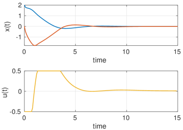
Figure 2: Closed-loop simulations of system (34) with the proposed MPC controller with $\nu=20$ and $N=100$. State (up) and input (down) trajectories.

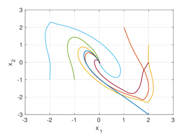
Figure 3: Phase portrait of the closed-loop system starting from various different initial points using $\nu=20$ and $N=100$.

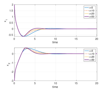
Figure 4: Responses for different approximation orders $\nu$ and fixed prediction horizon $N=100$.

5 Conclusions and future work directions

In this paper we proposed a tube-based MPC scheme for fractional systems which guarantees the satisfaction of state and input constraints. No assumptions on the fractional orders $\alpha_{i}$ were imposed other than that they be nonnegative, so the results presented here are valid also for non-commensurate systems. We make use of a linear and finite-dimensional approximation of the original dynamics and discuss how the order of approximation relates to the computational complexity and stability properties of the resulting controlled system. The proposed control methodology features two important stability properties: first, it converges exponentially fast to a convex neighbourhood of the origin and, second, under certain conditions the origin is an asymptotically stable equilibrium point of the controlled system.

In future work we will consider the discrepancy between the discrete-time fractional-order system and the original continuous-time system when the MPC control action is applied by a hold element. Only recently have such problems been solved for constrained linear time-invariant systems [40].

This work was funded by project 11$\Sigma\text{YN}$.10.1152, which is co-financed by the EU and Greece, Operational Program “Competitiveness & Entrepreneurship”, NSFR 2007-2013 in the context of GSRT National action “Cooperation”.

Appendix A Proof of Theorem 4

We hereafter assume, without any loss of generality, that the vector-norm $\|\cdot\|$ is the Euclidean norm and the matrix norm $\|\cdot\|$ is the corresponding induced norm.

(Part 1.: Attractivity) We take $\tilde{x}_{0}\in Z_{N}$ and we shall first prove that the controlled trajectory of the system starting from $\tilde{x}_{0}$ converges to the origin (attractivity). We start with an observation on the structure of $D_{\nu}$. First, we define the function $\Phi_{\nu}(M,\alpha)=\Psi_{\nu}(\alpha)-\Psi_{\nu+M}(\alpha)$ and notice that $D_{\nu}$ assumes the following decomposition

$$D_{\nu}=D_{\nu+M}\oplus\bigoplus_{i\in\mathbb{N}_{[1,l]}}\Phi_{\nu}(M,\alpha_{i})A^{\ast}_{i}X,$$

for any $M=1,2,\ldots$. Let $D^{0}=D_{\nu}$ and $S^{0}=S_{\infty}$. Choose any $\kappa\in(\epsilon,1)$ and take a $0<\theta_{0}<\min\{1,\frac{\kappa-\epsilon}{\epsilon}\sigma\}$ and, because of Theorem 3, there is a $k_{0}=k_{0}(\theta_{0})\in\mathbb{N}$ so that for all $k\geq k_{0}$, $\tilde{x}_{k}\in S^{0}\oplus\mathcal{B}^{\bar{n}}_{{}^{\theta_{0}}\!/_{2}}\subseteq\mathcal{B}^{\bar{n}}_{\sigma+\theta_{0}}$. Clearly, we may find $\eta_{0}>0$ is so that

$$\bigoplus_{j\in\mathbb{N}}A_{K}^{j}G\mathcal{B}_{\eta_{0}}\subseteq\mathcal{B}_{{}^{\epsilon\theta_{0}}\!/_{2}}^{\bar{n}},$$ (36)

and take $M_{0}\in\mathbb{N}$ so that $D_{\nu+M_{0}}\subseteq\mathcal{B}_{\eta_{0}}^{n}$ and let $k\geq k_{0}+\nu+M_{0}$; then, since $\tilde{x}_{k}\in\mathcal{B}^{\bar{n}}_{\sigma+{}^{\theta_{0}}\!/_{2}}$, we have that ${x}_{k-\nu-j}\in\mathcal{B}_{\sigma+{}^{\theta_{0}}\!/_{2}}^{n}$ for all $j\in\mathbb{N}_{[1,M_{0}]}$. Then, $d_{k}\in D^{1}$, where $D^{1}=\mathcal{B}_{\eta_{0}}\oplus\bigoplus_{i\in\mathbb{N}_{[1,l]}}\Phi_{\nu}(M_{0},\alpha_{i})A^{\ast}_{i}\mathcal{B}^{n}_{\sigma{+}\frac{\theta_{0}}{2}},$ and refine the new target set $S^{1}$ as follows using the following facts (i) for all $M$ and $\nu$ it is $\Phi_{\nu}(M,\alpha)\leq\Psi_{\nu}(\alpha)$ (ii) condition (28) (iii) inclusion (36) and (iv) because of our selection of $\theta_{0}$ it is $\epsilon(\theta_{0}+\sigma)<\kappa\sigma$.

$$S^{1} =\bigoplus_{j\in\mathbb{N}}A_{K}^{j}GD^{1}$$ (37)

$$=\bigoplus_{j\in\mathbb{N}}A_{K}^{j}G\mathcal{B}_{\eta_{0}}\oplus\bigoplus_{j\in\mathbb{N}}A_{K}^{j}G\bigoplus_{i\in\mathbb{N}_{[1,l]}}\Phi_{\nu}(M_{0},\alpha_{i})A^{\ast}_{i}\mathcal{B}^{n}_{\sigma{+}\frac{\theta_{0}}{2}}$$

$$\subseteq\mathcal{B}_{\epsilon\theta_{0}/2}^{\bar{n}}\oplus\bigoplus_{j\in\mathbb{N}}A_{K}^{j}G\bigoplus_{i\in\mathbb{N}_{[1,l]}}\Psi_{\nu}(\alpha_{i})A^{\ast}_{i}\mathcal{B}^{n}_{\sigma{+}\frac{\theta_{0}}{2}}$$

$$\subseteq\mathcal{B}_{\epsilon\frac{\theta_{0}}{2}}^{\bar{n}}\oplus\mathcal{B}_{\epsilon(\sigma+\frac{\theta_{0}}{2})}^{\bar{n}}\subseteq\mathcal{B}_{\epsilon(\sigma+\theta_{0})}^{\bar{n}}\subseteq\mathcal{B}_{\kappa\sigma}^{\bar{n}}$$ (38)

and the state will converge towards $S^{1}$. Choose $0<\theta_{1}<\kappa\theta_{0}$. There is a $k_{1}=k_{1}(\theta_{1})\in\mathbb{N}$ with $k_{1}>k_{0}$ so that $\tilde{x}_{k}\in S^{1}\oplus\mathcal{B}_{\theta_{1}/2}^{\bar{n}}$ (and of course $\tilde{x}_{k}\in\mathcal{B}_{\kappa\sigma+\theta_{1}/2}^{\bar{n}}$) for all $k\geq k_{1}$. Find $\eta_{1}>0$ with $\eta_{1}<\eta_{0}$ so that $\bigoplus_{j\in\mathbb{N}}A_{K}^{j}G\mathcal{B}_{\eta_{1}}^{\bar{n}}\subseteq\mathcal{B}_{\epsilon\theta_{1}/2}^{\bar{n}}$ and choose $M_{1}\in\mathbb{N}$ so that $D_{\nu+M_{1}}\subseteq\mathcal{B}_{\eta_{1}}^{n}$ and let $k\geq k_{1}+\nu+M_{1}$. Then, $x_{k-\nu-j}\in\mathcal{B}_{\kappa\sigma+\theta_{1}/2}^{n}$ for $j\in\mathbb{N}_{[1,M_{1}]}$. It follows that $d_{k}\in D^{2}$, where $D^{2}=\mathcal{B}_{\eta_{1}}\oplus\bigoplus_{i\in\mathbb{N}_{[1,l]}}\Phi_{\nu}(M_{1},\alpha_{i})A^{\ast}_{i}\mathcal{B}^{n}_{\kappa\sigma{+}\frac{\theta_{1}}{2}}$ and following the same procedure as for $S^{1}$ we have

$$S^{2}=\bigoplus_{j\in\mathbb{N}}A_{K}^{i}GD^{2}\subseteq\mathcal{B}_{\epsilon(\kappa\sigma+\theta_{1})}^{\bar{n}}\subseteq\mathcal{B}_{\kappa^{2}\sigma}^{\bar{n}}$$ (39)

Recursively, we construct a sequence of sets $\{S^{i}\}_{i\in\mathbb{N}}$ so that $S^{i}\subseteq\mathcal{B}_{\kappa^{i}\sigma}$ and for all $i\in\mathbb{N}$ it is $S^{i}\ni 0$, therefore $S^{i}\to\{0\}$ as $i\to\infty$ and, as a result, $\tilde{x}_{k}\to 0$ as it follows from [31, Ex. 4.3(c)].

(Part 2.: Stability) We now need to show that the origin is stable, that is, we need to prove that for every $\epsilon>0$ there is a $\delta=\delta(\epsilon)>0$ so that $\|\tilde{x}_{k}\|<\epsilon$ for all $k\in\mathbb{N}$ whenever $\|\tilde{x}_{0}\|<\delta$ (and $\tilde{x}_{0}\in Z_{N}$) . First, notice that $\|x\|<\delta$ implies $\mathrm{dist}(x,S^{i})<\delta$. By Theorem 3 we know that for each $i\in\mathbb{N}$ and given $\epsilon$ there is a $\delta^{\ast}={\delta}^{\ast}(\epsilon,i)$ so that $\mathrm{dist}(x_{0},S^{i})<{\delta}^{\ast}$ implies $\mathrm{dist}(x_{k},S^{i})<{}^{\epsilon}\!/_{2}$ for all $k\in\mathbb{N}$.

Let $i=i(\epsilon)=\lceil\log_{\kappa}\frac{\epsilon}{2\sigma}\rceil$ and take $x_{0}$ so that $\|x_{0}\|<\delta(\epsilon,i(\epsilon))$; then $\mathrm{dist}(x_{0},S^{i})<\delta(\epsilon,i(\epsilon))$, therefore for all $k\in\mathbb{N}$, $\mathrm{dist}(x_{k},S^{i})<\frac{\epsilon}{2}$ and $\|x_{k}\|<\frac{\epsilon}{2}+\kappa^{i}\sigma<\epsilon$.   $\square$

Appendix B Properties of $\mathrm{p}[S]$ and $\mathrm{p}[S\cap L_{i}]$

Let $\beta=\max_{s\in S}\|s\|$. Then $S\subseteq\mathcal{B}_{\beta}$, thus for all $\tilde{x}\in\mathbb{R}^{\bar{n}}$, $\mathrm{p}[S](x)\geq\mathrm{p}[\mathcal{B}_{\beta}^{\bar{n}}](\tilde{x})$, i.e., $\mathrm{p}[S](\tilde{x})\geq\frac{\|\tilde{x}\|}{\beta}$, or equivalently $\|\tilde{x}\|\leq\beta\mathrm{p}[S](\tilde{x})$. Given that $S\cap L_{i}$ has nonempty interior, we may find $\gamma_{i}>0$ with $\mathcal{B}_{\gamma_{i}}^{n}\subseteq S\cap L_{i}$. Let $x$ be the projection of $\tilde{x}$ on $L_{i}$. We then have $\mathcal{B}^{n}_{\gamma_{i}}\subseteq S\cap L_{i}$, thus $\mathrm{p}[S\cap L_{i}](x)\leq\mathrm{p}[\mathcal{B}_{\gamma_{i}}^{n}](x)=\frac{\|x\|}{\gamma_{i}}$. We then have $\gamma_{i}\mathrm{p}[S\cap L_{i}](x)\leq\|x\|\leq\|\tilde{x}\|\leq\beta\mathrm{p}[S](\tilde{x})$ therefore $\mathrm{p}[S\cap L_{i}](x)\leq a_{i}\mathrm{p}[S](\tilde{x}),$ with $a_{i}=\frac{\beta}{\gamma_{i}}$.  $\square$

References

- [1] D. Boudjehem and B. Boudjehem. The use of fractional order models in predictive control. In 3 Conference on Nonlinear Science and Complexity, symposium: Fractional Calculus Applications, Ankara, Turkey, July 2010.
- [2] S. Boyd and L. Vandenberghe. Convex Optimization. Cambridge university press, Cambridge, 7th edition edition, 2009.
- [3] M. Busłowicz and T. Kaczorek. Simple conditions for practical stability of positive fractional discrete-time linear systems. Int. J. Appl. Math. Comput. Sci., 19(2):263–269, 2009.
- [4] T. Clarke, B.N. Narahari Achar, and J.W. Hanneken. Mittag–Leffler functions and transmission lines. Journal of Molecular Liquids, 114(1–3):159 – 163, 2004.
- [5] Z. Deng, H. Cao, X. Li, J. Jiang, J. Yang, and Y. Qin. Generalized predictive control for fractional order dynamic model of solid oxide fuel cell output power. Journal of Power Sources, 195(24):8097 – 8103, 2010.
- [6] M. Diehl and J. Bjornberg. Robust dynamic programming for min-max model predictive control of constrained uncertain systems. Automatic Control, IEEE Transactions on, 49(12):2253–2257, Dec 2004.
- [7] A. Dokoumetzidis and P. Macheras. IVIVC of controlled release formulations: Physiological-dynamical reasons for their failure. Journal of Controlled Release, 129(2):76–78, 2008.
- [8] A. Dokoumetzidis and P. Macheras. The changing face of the rate concept in biopharmaceutical sciences: From classical to fractal and finally to fractional. Pharmaceutical Research, 28(5):1229–1232, 2011.
- [9] A. Dokoumetzidis, R. Magin, and P. Macheras. Fractional kinetics in multi-compartmental systems. Journal of Pharmacokinetics and Pharmacodynamics, 37(5):507–524, 2010.
- [10] G.-R. Duan. Analysis and Design of Descriptor Linear Systems. Springer New York, 2010.
- [11] P. Gritzmann and B. Sturmfels. Minkowski addition of polytopes: Computational complexity and applications to Gröbner basis. SIAM J. Discrete Math., 6(2):246–269, 1993.
- [12] S. Guermah, S. Djennoune, and M. Bettayeb. A new approach for stability analysis of linear discrete-time fractional-order systems. In D. Baleanu, Z.B. Guvenc, and J.A.T. Machado, editors, New Trends in Nanotechnology and Fractional Calculus Applications, pages 151–162. Springer Netherlands, 2010.
- [13] S. Guerman, S. Djennoune, and M. Bettayeb. Discrete-time fractional-order systems: Modeling and stability issues. In M.S. Mahmoud, editor, Advances in discrete-time systems. Intech publications, 2012.
- [14] G. Guo, K. Li, and Y. Wang. Exact solutions of a modified fractional diffusion equation in the finite and semi-infinite domains. Physica A: Statistical Mechanics and its Applications, 417(1):193 – 201, 2015.
- [15] R. Hilfer. Applications of Fractional Calculus in Physics. World Scientific, Singapore, 2000.
- [16] M.M. Joshi, V.A. Vyawahare, and M.D. Patil. Model predictive control for fractional-order system a modeling and approximation based analysis. In Simulation and Modeling Methodologies, Technologies and Applications (SIMULTECH), 2014 International Conference on, pages 361–372, Aug 2014.
- [17] A.B. Kurzhanski and I.V Alyi. Ellipsoidal Calculus for Estimation and Control. Birkhhäuser, Boston, 1997.
- [18] J. Kytariolos, A. Dokoumetzidis, and P. Macheras. Power law IVIVC: An application of fractional kinetics for drug release and absorption. European Journal of Pharmaceutical Sciences, 41(2):299–304, 2010.
- [19] J. Löfberg. Yalmip : A toolbox for modeling and optimization in MATLAB. In Proceedings of the CACSD Conference, Taipei, Taiwan, 2004.
- [20] R. Magin, M.D. Ortigueira, I. Podlubny, and J. Trujillo. On the fractional signals and systems. Signal Processing, 91(3):350 – 371, 2011.
- [21] R.L. Magin. Fractional calculus models of complex dynamics in biological tissues. Computers & Mathematics with Applications, 59(5):1586–1593, 2010.
- [22] D.Q. Mayne, J.B. Rawlings, C.V. Rao, and P.O.M. Scokaert. Constrained model predictive control: Stability and optimality. Automatica, 36:789–814, 2000.
- [23] F. Mesquine, A. Hmamed, M. Benhayoun, A. Benzaouia, and F. Tadeo. Robust stabilization of constrained uncertain continuous-time fractional positive systems. Journal of the Franklin Institute, 352(1):259–270, 2015.
- [24] M.D. Ortigueira, F.J.V. Coito, and J.J. Trujillo. Discrete-time differential systems. Signal Processing, 107:198–217, 2015.
- [25] L.M. Pereira. Fractal pharmacokinetics. Comput Math Methods Med., 11:161–184, 2010.
- [26] I. Podlubny. Fractional differential equations, volume 198 of Mathematics in Science and Engineering. Academic Publisher, San Diego, California, 1999.
- [27] S.V. Raković, E.C. Kerrigan, K.I. Kouramas, and D.Q. Mayne. Invariant approximations of the minimal robust positively invariant set. IEEE Transactions on Automatic Control, 50(3):406–410, March 2005.
- [28] J. B. Rawlings and D. Q. Mayne. Model Predictive Control: Theory and Design. Nob Hill Publishing, 2009.
- [29] A. Rhouma and F. Bouani. Robust model predictive control of uncertain fractional systems: a thermal application. IET Control Theory Applications, 8(17):1986–1994, 2014.
- [30] A. Rhouma, B. Bouzouita, and F. Bouani. Model predictive control of fractional systems using numerical approximation. In Computer Applications Research (WSCAR), 2014 World Symposium on, pages 1–6, Jan 2014.
- [31] R.T. Rockafellar and R. J.-B. Wets. Variational Analysis. Grundlehren der mathematischen Wissenschaften. Springer, Dordrecht, 1998.
- [32] M. Romero, Á.P. de Madrid, C. Mañoso, and R.H. Berlinches. Generalized predictive control of arbitrary real order. In D. Baleanu, Z.B. Guvenc, and J.A.T. Machado, editors, New Trends in Nanotechnology and Fractional Calculus Applications, pages 411–418. Springer Netherlands, 2010.
- [33] M. Romero, Á.P. de Madrid, C. Mañoso, V. Milanés, and B.M. Vinagre. Fractional-order generalized predictive control: Application for low-speed control of gasoline-propelled cars. Mathematical Problems in Engineering, 2013:1–10, 2013. Article ID 895640.
- [34] M. Romero, Á.P. de Madrid, C. Mañoso, and B.M. Vinagre. Fractional-order generalized predictive control: Formulation and some properties. In Control Automation Robotics Vision (ICARCV), 2010 11th International Conference on, pages 1495–1500, Dec 2010.
- [35] M. Romero, Á.P. de Madrid, C. Mañoso, and B.M. Vinagre. A survey of fractional-order generalized predictive control. In Decision and Control (CDC), 2012 IEEE 51st Annual Conference on, pages 6867–6872, Dec 2012.
- [36] M. Romero, I. Tejado, J.I. Suárez, B.M. Vinagre, and Á.P. de Madrid. GPC strategies for the lateral control of a networked AGV. In Proc. IEEE Int. Conf. Mechatronics, 2009.
- [37] S. Samko, A. Kilbas, and O. Marichev. Fractional integral and derivatives. Gordon & Breach Science Publishers, 1993.
- [38] I. Schäfer and K. Krüger. Modelling of coils using fractional derivatives. Journal of Magnetism and Magnetic Materials, 307(1):91 – 98, 2006.
- [39] P. Sopasakis, S. Ntouskas, and H. Sarimveis. Robust model predictive control for discrete-time fractional-order systems. In Control and Automation (MED), 2015 23th Mediterranean Conference on, pages 384–389, June 2015.
- [40] P. Sopasakis, P. Patrinos, and H. Sarimveis. MPC for sampled-data linear systems: Guaranteeing continuous-time positive invariance. IEEE Trans. Auto. Contr., 59(4):1088–1093, 2013.
- [41] P. Sopasakis and H. Sarimveis. Controlled drug administration by a fractional PID. In 19th IFAC World Congress, pages 8421–8426, Cape Town, South Africa, August 2014.
- [42] V. Tarasov. Fractional Dynamics – Applications of Fractional Calculus to Dynamics of Particles, Fields and Media. Nonlinear Physical Science. Springer, Heidelberg, 2010.
- [43] B.M. Vinagre, I. Podlubny, A. Hernandez, and V. Feliu. Some approximations of fractional order operators used in control theory and applications. Fractional calculus and applied analysis, 3(3):231–248, 2000.