Relativistic hydrodynamics in heavy-ion collisions: general aspects and recent developments

Abstract

Relativistic hydrodynamics has been quite successful in explaining the collective behaviour of the QCD matter produced in high energy heavy-ion collisions at RHIC and LHC. We briefly review the latest developments in the hydrodynamical modeling of relativistic heavy-ion collisions. Essential ingredients of the model such as the hydrodynamic evolution equations, dissipation, initial conditions, equation of state, and freeze-out process are reviewed. We discuss observable quantities such as particle spectra and anisotropic flow and effect of viscosity on these observables. Recent developments such as event-by-event fluctuations, flow in small systems (proton-proton and proton-nucleus collisions), flow in ultra central collisions, longitudinal fluctuations and correlations and flow in intense magnetic field are also discussed.

I Introduction

The existence of both confinement and asymptotic freedom in Quantum Chromodynamics (QCD) has led to many speculations about its thermodynamic and transport properties. Due to confinement, the nuclear matter must be made of hadrons at low energies, hence it is expected to behave as a weakly interacting gas of hadrons. On the other hand, at very high energies asymptotic freedom implies that quarks and gluons interact only weakly and the nuclear matter is expected to behave as a weakly coupled gas of quarks and gluons. In between these two configurations there must be a phase transition where the hadronic degrees of freedom disappear and a new state of matter, in which the quark and gluon degrees of freedom manifest directly over a certain volume, is formed. This new phase of matter, referred to as Quark-Gluon Plasma (QGP), is expected to be created when sufficiently high temperatures or densities are reached Lee ; Collins:1974ky ; Itoh:1970uw .

The QGP is believed to have existed in the very early universe (a few microseconds after the Big Bang), or some variant of which possibly still exists in the inner core of a neutron star where it is estimated that the density can reach values ten times higher than those of ordinary nuclei. It was conjectured theoretically that such extreme conditions can also be realized on earth, in a controlled experimental environment, by colliding two heavy nuclei with ultra-relativistic energies Baumgardt:1975qv . This may transform a fraction of the kinetic energies of the two colliding nuclei into heating the QCD vacuum within an extremely small volume where temperatures million times hotter than the core of the sun may be achieved.

With the advent of modern accelerator facilities, ultra-relativistic heavy-ion collisions have provided an opportunity to systematically create and study different phases of the bulk nuclear matter. It is widely believed that the QGP phase is formed in heavy-ion collision experiments at Relativistic Heavy-Ion Collider (RHIC) located at Brookhaven National Laboratory, USA and Large Hadron Collider (LHC) at European Organization for Nuclear Research (CERN), Geneva. A number of indirect evidences found at the Super Proton Synchrotron (SPS) at CERN, strongly suggested the formation of a “new state of matter” CERN , but quantitative and clear results were only obtained at RHIC energies Tannenbaum:2006ch ; Kolb ; Gyulassy ; Tomasik ; Muller ; Arsene:2004fa ; Adcox:2004mh ; Back:2004je ; Adams:2005dq , and recently at LHC energies Aamodt:2010pa ; Aamodt:2010pb ; Aamodt:2010cz ; ALICE:2011ab . The regime with relatively large baryon chemical potential will be probed by the upcoming experimental facilities like Facility for Anti-proton and Ion Research (FAIR) at GSI, Darmstadt. An illustration of the QCD phase diagram and the regions probed by these experimental facilities is shown in Fig. 1 gsi.de .

It is possible to create hot and dense nuclear matter with very high energy densities in relatively large volumes by colliding ultra-relativistic heavy ions. In these conditions, the nuclear matter created may be close to (local) thermodynamic equilibrium, providing the opportunity to investigate the various phases and the thermodynamic and transport properties of QCD. It is important to note that, even though it appears that a deconfined state of matter is formed in these colliders, investigating and extracting the transport properties of QGP from heavy-ion collisions is not an easy task since it cannot be observed directly. Experimentally, it is only feasible to measure energy and momenta of the particles produced in the final stages of the collision, when nuclear matter is already relatively cold and non-interacting. Hence, in order to study the thermodynamic and transport properties of the QGP, the whole heavy-ion collision process from the very beginning till the end has to be modelled: starting from the stage where two highly Lorentz contracted heavy nuclei collide with each other, the formation and thermalization of the QGP or de-confined phase in the initial stages of the collision, its subsequent space-time evolution, the phase transition to the hadronic or confined phase of matter, and eventually, the dynamics of the cold hadronic matter formed in the final stages of the collision. The different stages of ultra-relativistic heavy-ion collisions are schematically illustrated in Fig. 2 duke.edu .

Assuming that thermalization is achieved in the early stages of heavy-ion collisions and that the interaction between the quarks is strong enough to maintain local thermodynamic equilibrium during the subsequent expansion, the time evolution of the QGP and hadronic matter can be described by the laws of fluid dynamics Stoecker:1986ci ; Rischke:1995ir ; Rischke:1995mt ; Shuryak:2003xe . Fluid dynamics, also loosely referred to as hydrodynamics, is an effective approach through which a system can be described by macroscopic variables, such as local energy density, pressure, temperature and flow velocity. The most appealing feature of fluid dynamics is the fact that it is simple and general. It is simple in the sense that all the information of the system is contained in its thermodynamic and transport properties, i.e., its equation of state and transport coefficients. Fluid dynamics is also general because it relies on only one assumption: the system remains close to local thermodynamic equilibrium throughout its evolution. Although the hypothesis of proximity to local equilibrium is quite strong, it saves us from making any further assumption regarding the description of the particles and fields, their interactions, the classical or quantum nature of the phenomena involved etc. Hydrodynamic analysis of the spectra and azimuthal anisotropy of particles produced in heavy-ion collisions at RHIC Romatschke:2007mq ; Song:2010mg and recently at LHC Luzum:2010ag ; Qiu:2011hf suggests that the matter formed in these collisions is strongly-coupled quark-gluon plasma (sQGP).

Figure 1: (Color online) Schematic phase diagram of the QCD matter. The net baryon density on x-axis is normalized to that of the normal nuclear matter gsi.de .

Application of viscous hydrodynamics to high-energy heavy-ion collisions has evoked widespread interest ever since a surprisingly small value of $\eta/s$ was estimated from the analysis of the elliptic flow data Romatschke:2007mq . It is interesting to note that in the strong coupling limit of a large class of holographic theories, the value of the shear viscosity to entropy density ratio $\eta/s=1/4\pi$. Kovtun, Son and Starinets (KSS) conjectured this strong coupling result to be the absolute lower bound for all fluids, i.e., $\eta/s\geq 1/4\pi$ Policastro:2001yc ; Kovtun:2004de . This specific combination of hydrodynamic quantities, $\eta/s$, accounts for the difference between momentum and charge diffusion such that even though the diffusion constant goes to zero in the strong coupling limit, the ratio $\eta/s$ remains finite Schaefer:2014awa . Similar result for a lower bound also follows from the quantum mechanical uncertainty principle. The kinetic theory prediction for viscosity, $\eta=\frac{1}{3}nl_{\rm mfp}\bar{p}$, suggests that low viscosity corresponds to short mean free path. On the other hand, the uncertainty relation implies that the product of the mean free path and the average momentum cannot be arbitrarily small, i.e., $l_{\rm mfp}\bar{p}\gtrsim 1$. For a weakly interacting relativistic Bose gas, the entropy per particle is given by $s/n=3.6$. This leads to $\eta/s\gtrsim 0.09$ which is very close to the lower KSS bound.

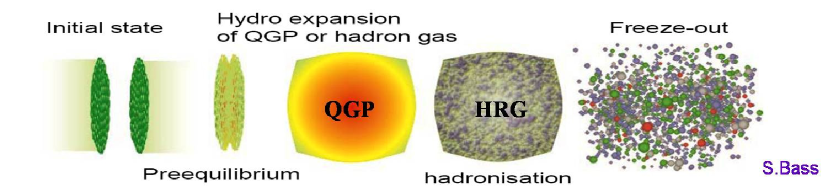
Figure 2: (Color online) Various stages of ultra-relativistic heavy-ion collisions duke.edu .

Indeed the estimated $\eta/s$ of QGP was so close to the KSS bound that it led to the claim that the matter formed at RHIC was the most perfect fluid ever observed. A precise estimate of $\eta/s$ is vital to the understanding of the properties of the QCD matter and is presently a topic of intense investigation, see Chaudhuri:2013yna and references therein for more details. In this review, we shall discuss the general aspects of the formulation of relativistic fluid dynamics and its application to the physics of high-energy heavy-ion collisions. Along with these general concepts we shall also discuss here some of the recent developments in the field. Among the recent developments the most striking feature is the experimental observation of flow like pattern in the particle azimuthal distribution of high multiplicity proton-proton (p-p) and proton-lead (p-Pb)collisions. We will discuss in this review the success of hydrodynamics model in describing these recent experimental measurements by assuming hydrodynamics flow of small systems.

The review is organised as follows, In section II we discuss the general formalism of a causal theory of relativistic dissipative fluid dynamics. Section III deals with the initial conditions necessary for the modeling of relativistic heavy-ion, p-p and p-Pb collisions. In section IV, we discuss some models of pre-equilibrium dynamics employed before hydrodynamic evolution. Section V briefly covers various equations of state, necessary to close the hydrodynamic equations. In section VI, particle production mechanism via Cooper-Frye freeze-out and anisotropic flow generation is discussed. In Section VII, we discuss models of hadronic rescattering after freeze-out and contribution to particle spectra and flow from resonance decays. Section VIII deals with the extraction of transport coefficients from hydrodynamic analysis of flow data. Finally, in section IX, we discuss recent developments in the hydrodynamic modeling of relativistic collisions.

In this review, unless stated otherwise, all physical quantities are expressed in terms of natural units, where, $\hbar=c=k_{\rm B}=1$, with $\hbar=h/2\pi$, where $h$ is the Planck constant, $c$ the velocity of light in vacuum, and $k_{\rm B}$ the Boltzmann constant. Unless stated otherwise, the spacetime is always taken to be Minkowskian where the metric tensor is given by $g_{\mu\nu}=\mbox{diag}(+1,-1,-1,-1)$. Apart from Minkowskian coordinates $x^{\mu}=(t,x,y,z)$, we will also regularly employ Milne coordinate system $x^{\mu}=(\tau,x,y,\eta_{s})$ or $x^{\mu}=(\tau,r,\varphi,\eta_{s})$, with proper time $\tau=\sqrt{t^{2}-z^{2}}$, the radial coordinate $r=\sqrt{x^{2}+y^{2}}$, the azimuthal angle $\varphi=\tan^{-1}(y/x)$, and spacetime rapidity $\eta_{s}=\tanh^{-1}(z/t)$. Hence, $t=\tau\cosh\eta_{s}$, $x=r\cos\varphi$, $y=r\sin\varphi$, and $z=\tau\sinh\eta_{s}$. For the coordinate system $x^{\mu}=(\tau,x,y,\eta_{s})$, the metric becomes $g_{\mu\nu}=\mbox{diag}(1,-1,-1,-\tau^{2})$, whereas for $x^{\mu}=(\tau,r,\varphi,\eta_{s})$, the metric is $g_{\mu\nu}=\mbox{diag}(1,-1,-r^{2},-\tau^{2})$. Roman letters are used to indicate indices that vary from 1-3 and Greek letters for indices that vary from 0-3. Covariant and contravariant four-vectors are denoted as $p_{\mu}$ and $p^{\mu}$, respectively. The notation $p\cdot q\equiv p_{\mu}q^{\mu}$ represents scalar product of a covariant and a contravariant four-vector. Tensors without indices shall always correspond to Lorentz scalars. We follow Einstein summation convention, which states that repeated indices in a single term are implicitly summed over all the values of that index.

We denote the fluid four-velocity by $u^{\mu}$ and the Lorentz contraction factor by $\gamma$. The projector onto the space orthogonal to $u^{\mu}$ is defined as: $\Delta^{\mu\nu}\equiv g^{\mu\nu}-u^{\mu}u^{\nu}$. Hence, $\Delta^{\mu\nu}$ satisfies the conditions $\Delta^{\mu\nu}u_{\mu}=\Delta^{\mu\nu}u_{\nu}=0$ with trace $\Delta^{\mu}_{\mu}=3$. The partial derivative $\partial^{\mu}$ can then be decomposed as:

$$\partial^{\mu}=\nabla^{\mu}+u^{\mu}D,~{}~{}\mathrm{where}~{}~{}\nabla^{\mu}\equiv\Delta^{\mu\nu}\partial_{\nu}~{}~{}\mathrm{and}~{}~{}D\equiv u^{\mu}\partial_{\mu}.$$

In the fluid rest frame, $D$ reduces to the time derivative and $\nabla^{\mu}$ reduces to the spacial gradient. Hence, the notation $\dot{f}\equiv Df$ is also commonly used. We also frequently use the symmetric, anti-symmetric and angular brackets notations defined as

$$A_{(\mu}B_{\nu)} \equiv \frac{1}{2}\left(A_{\mu}B_{\nu}+A_{\nu}B_{\mu}\right),$$

$$A_{[\mu}B_{\nu]} \equiv \frac{1}{2}\left(A_{\mu}B_{\nu}-A_{\nu}B_{\mu}\right),$$

$$A_{\langle\mu}B_{\nu\rangle} \equiv \Delta^{\alpha\beta}_{\mu\nu}A_{\alpha}B_{\beta}.$$

where,

$$\Delta^{\alpha\beta}_{\mu\nu}\equiv\frac{1}{2}\left(\Delta^{\alpha}_{\mu}\Delta^{\beta}_{\nu}+\Delta^{\alpha}_{\nu}\Delta^{\beta}_{\mu}-\frac{2}{3}\Delta^{\alpha\beta}\Delta_{\mu\nu}\right)$$

is the traceless symmetric projection operator orthogonal to $u^{\mu}$ satisfying the conditions $\Delta^{\alpha\beta}_{\mu\nu}\Delta_{\alpha\beta}=\Delta^{\alpha\beta}_{\mu\nu}\Delta^{\mu\nu}=0$.

II Relativistic fluid dynamics

The physical characterization of a system consisting of many degrees of freedom is in general a non-trivial task. For instance, the mathematical formulation of a theory describing the microscopic dynamics of a system containing a large number of interacting particles is one of the most challenging problems of theoretical physics. However, it is possible to provide an effective macroscopic description, over large distance and time scales, by taking into account only the degrees of freedom that are relevant at these scales. This is a consequence of the fact that on macroscopic distance and time scales the actual degrees of freedom of the microscopic theory are imperceptible. Most of the microscopic variables fluctuate rapidly in space and time, hence only average quantities resulting from the interactions at the microscopic level can be observed on macroscopic scales. These rapid fluctuations lead to very small changes of the average values, and hence are not expected to contribute to the macroscopic dynamics. On the other hand, variables that do vary slowly, such as the conserved quantities, are expected to play an important role in the effective description of the system. Fluid dynamics is one of the most common examples of such a situation. It is an effective theory describing the long-wavelength, low frequency limit of the underlying microscopic dynamics of a system.

A fluid is defined as a continuous system in which every infinitesimal volume element is assumed to be close to thermodynamic equilibrium and to remain near equilibrium throughout its evolution. Hence, in other words, in the neighbourhood of each point in space, an infinitesimal volume called fluid element is defined in which the matter is assumed to be homogeneous, i.e., any spatial gradients can be ignored, and is described by a finite number of thermodynamic variables. This implies that each fluid element must be large enough, compared to the microscopic distance scales, to guarantee the proximity to thermodynamic equilibrium, and, at the same time, must be small enough, relative to the macroscopic distance scales, to ensure the continuum limit. The co-existence of both continuous (zero volume) and thermodynamic (infinite volume) limits within a fluid volume might seem paradoxical at first glance. However, if the microscopic and the macroscopic length scales of the system are sufficiently far apart, it is always possible to establish the existence of a volume that is small enough compared to the macroscopic scales, and at the same time, large enough compared to the microscopic ones. Here, we will assume the existence of a clear separation between microscopic and macroscopic scales to guarantee the proximity to local thermodynamic equilibrium.

Relativistic fluid dynamics has been quite successful in explaining the various collective phenomena observed in astrophysics, cosmology and the physics of high-energy heavy-ion collisions. In cosmology and certain areas of astrophysics, one needs a fluid dynamics formulation consistent with the General Theory of Relativity Ibanez . On the other hand, a formulation based on the Special Theory of Relativity is quite adequate to treat the evolution of the strongly interacting matter formed in high-energy heavy-ion collisions when it is close to a local thermodynamic equilibrium. In fluid dynamical approach, although no detailed knowledge of the microscopic dynamics is needed, however, knowledge of the equation of state relating pressure, energy density and baryon density is required. The collective behaviour of the hot and dense quark-gluon plasma created in ultra-relativistic heavy-ion collisions has been studied quite extensively within the framework of relativistic fluid dynamics. In application of fluid dynamics, it is natural to first employ the simplest version which is ideal hydrodynamics which neglects the viscous effects and assumes that local equilibrium is always perfectly maintained during the fireball expansion. Microscopically, this requires that the microscopic scattering time be much shorter than the macroscopic expansion (evolution) time. In other words, ideal hydrodynamics assumes that the mean free path of the constituent particles is much smaller than the system size. However, as all fluids are dissipative in nature due to the quantum mechanical uncertainty principle Danielewicz:1984ww , the ideal fluid results serve only as a benchmark when dissipative effects become important.

When discussing the application of relativistic dissipative fluid dynamics to heavy-ion collision, one is faced with yet another predicament: the theory of relativistic dissipative fluid dynamics is not yet conclusively established. In fact, introducing dissipation in relativistic fluids is not at all a trivial task and still remains one of the important topics of research in high-energy physics. Ideal hydrodynamics assumes that local thermodynamic equilibrium is perfectly maintained and each fluid element is homogeneous, i.e., spatial gradients are absent (zeroth order in gradient expansion). If this is not satisfied, dissipative effects come into play. The earliest theoretical formulations of relativistic dissipative hydrodynamics also known as first-order theories, are due to Eckart Eckart:1940zz and Landau-Lifshitz Landau . However, these formulations, collectively called relativistic Navier-Stokes (NS) theory, suffer from acausality and numerical instability. The reason for the acausality is that in the gradient expansion the dissipative currents are linearly proportional to gradients of temperature, chemical potential, and velocity, resulting in parabolic equations. Thus, in Navier-Stokes theory the gradients have an instantaneous influence on the dissipative currents. Such instantaneous effects tend to violate causality and cannot be allowed in a covariant setup, leading to the instabilities investigated in Refs. Hiscock:1983zz ; Hiscock:1985zz ; Hiscock:1987zz .

The second-order Israel-Stewart (IS) theory Israel:1979wp , restores causality but may not guarantee stability Huovinen:2008te . The acausality problems were solved by introducing a time delay in the creation of the dissipative currents from gradients of the fluid-dynamical variables. In this case, the dissipative quantities become independent dynamical variables obeying equations of motion that describe their relaxation towards their respective Navier-Stokes values. The resulting equations are hyperbolic in nature which preserves causality. Israel-Stewart theory has been widely applied to ultra-relativistic heavy-ion collisions in order to describe the time evolution of the QGP and the subsequent freeze-out process of the hadron resonance gas. Although IS hydrodynamics has been quite successful in modelling relativistic heavy-ion collisions, there are several inconsistencies and approximations in its formulation which prevent proper understanding of the thermodynamic and transport properties of the QGP. Moreover, the second-order IS theory can be derived in several ways, each leading to a different set of transport coefficients. Therefore, in order to quantify the transport properties of the QGP from experiment and confirm the claim that it is indeed the most perfect fluid ever created, the theoretical foundations of relativistic dissipative fluid dynamics must be first addressed and clearly understood. In this section, we review the basic aspects of thermodynamics and discuss the formulation of relativistic fluid dynamics from a phenomenological perspective. The salient features of kinetic theory in the context of fluid dynamics will also be discussed.

II.1 Thermodynamics

Thermodynamics is an empirical description of the macroscopic or large-scale properties of matter and it makes no hypotheses about the small-scale or microscopic structure. It is concerned only with the average behaviour of a very large number of microscopic constituents, and its laws can be derived from statistical mechanics. A thermodynamic system can be described in terms of a small set of extensive variables, such as volume ($V$), the total energy ($E$), entropy ($S$), and number of particles ($N$), of the system. Thermodynamics is based on four phenomenological laws that explain how these quantities are related and how they change with time Fermi ; Reif ; Reichl .

• Zeroth Law: If two systems are both in thermal equilibrium with a third system then they are in thermal equilibrium with each other. This law helps define the notion of temperature.

• First Law: All the energy transfers must be accounted for to ensure the conservation of the total energy of a thermodynamic system and its surroundings. This law is the principle of conservation of energy.

• Second Law: An isolated physical system spontaneously evolves towards its own internal state of thermodynamic equilibrium. Employing the notion of entropy, this law states that the change in entropy of a closed thermodynamic system is always positive or zero.

• Third Law: Also known an Nernst’s heat theorem, states that the difference in entropy between systems connected by a reversible process is zero in the limit of vanishing temperature. In other words, it is impossible to reduce the temperature of a system to absolute zero in a finite number of operations.

The first law of thermodynamics postulates that the changes in the total energy of a thermodynamic system must result from: (1) heat exchange, (2) the mechanical work done by an external force, and (3) from particle exchange with an external medium. Hence the conservation law relating the small changes in state variables, $E$, $V$, and $N$ is

$$\delta E=\delta Q-P\delta V+\mu\,\delta N,$$ (1)

where $P$ and $\mu$ are the pressure and chemical potential, respectively, and $\delta Q$ is the amount of heat exchange.

The heat exchange takes into account the energy variations due to changes of internal degrees of freedom that are not described by the state variables. The heat itself is not a state variable since it can depend on the past evolution of the system and may take several values for the same thermodynamic state. However, when dealing with reversible processes (in time), it becomes possible to assign a state variable related to heat. This variable is the entropy, $S$ , and is defined in terms of the heat exchange as $\delta Q=T\delta S$, with the temperature $T$ being the proportionality constant. Then, when considering variations between equilibrium states that are infinitesimally close to each other, it is possible to write the first law of thermodynamics in terms of differentials of the state variables,

$$dE=TdS-PdV+\mu\,dN.$$ (2)

Hence, using Eq. (2), the intensive quantities, $T$, $\mu$ and $P$, can be obtained in terms of partial derivatives of the entropy as

$$\left.{\frac{\partial S}{\partial E}}\right|_{N,V}=\frac{1}{T},\qquad\left.{\frac{\partial S}{\partial V}}\right|_{N,E}=\frac{P}{T},\qquad\left.{\frac{\partial S}{\partial N}}\right|_{E,V}=-\frac{\mu}{T}.$$ (3)

The entropy is mathematically defined as an extensive and additive function of the state variables, which means that

$$S(\lambda E,\lambda V,\lambda N)=\lambda S(E,V,N).$$ (4)

Differentiating both sides with respect to $\lambda$, we obtain

$$S=E\left.{\frac{\partial S}{\partial\lambda E}}\right|_{\lambda N,\lambda V}+V\left.{\frac{\partial S}{\partial\lambda V}}\right|_{\lambda N,\lambda E}+N\left.{\frac{\partial S}{\partial\lambda N}}\right|_{\lambda E,\lambda V},$$ (5)

which holds for any arbitrary value of $\lambda$. Setting $\lambda=1$ and using Eq. (3), we obtain the so-called Euler’s relation

$$E=-PV+TS+\mu\,N.$$ (6)

Using Euler’s relation, Eq. (6), along with the first law of thermodynamics, Eq. (2), we arrive at the Gibbs-Duhem relation

$$VdP=SdT+Nd\mu.$$ (7)

In terms of energy, entropy and number densities defined as $\epsilon\equiv E/V$, $s\equiv S/V$, and $n\equiv N/V$ respectively, the Euler’s relation, Eq. (6) and Gibbs-Duhem relation, Eq. (7), reduce to

$$\epsilon =-P+Ts+\mu\,n$$ (8)

$$dP =s\,dT+n\,d\mu.$$ (9)

Differentiating Eq. (8) and using Eq. (9), we obtain the relation analogous to first law of thermodynamics

$$d\epsilon=Tds+\mu\,dn\quad\Rightarrow\quad ds=\frac{1}{T}\,d\epsilon-\frac{\mu}{T}\,dn.$$ (10)

It is important to note that all the densities defined above $(\epsilon,~{}s,~{}n)$ are intensive quantities.

The equilibrium state of a system is defined as a stationary state where the extensive and intensive variables of the system do not change. We know from the second law of thermodynamics that the entropy of an isolated thermodynamic system must either increase or remain constant. Hence, if a thermodynamic system is in equilibrium, the entropy of the system being an extensive variable, must remain constant. On the other hand, for a system that is out of equilibrium, the entropy must always increase. This is an extremely powerful concept that will be extensively used in this section to constrain and derive the equations of motion of a dissipative fluid. This concludes a brief outline of the basics of thermodynamics; for a more detailed review, see Ref. Reichl . In the next section, we introduce and derive the equations of relativistic ideal fluid dynamics.

II.2 Relativistic ideal fluid dynamics

An ideal fluid is defined by the assumption of local thermal equilibrium, i.e., all fluid elements must be exactly in thermodynamic equilibrium Landau ; Weinberg . This means that at each space-time coordinate of the fluid $x\equiv x^{\mu}$, there can be assigned a temperature $T(x)$, a chemical potential $\mu(x)$, and a collective four-velocity field,

$$u^{\mu}(x)\equiv\frac{dx^{\mu}}{d\tau}.$$ (11)

The proper time increment $d\tau$ is given by the line element

$$(d\tau)^{2}=g_{\mu\nu}dx^{\mu}dx^{\nu}=(dt)^{2}-(d\vec{x})^{2}=(dt)^{2}\left[1-(\vec{v})^{2}\right],$$ (12)

where $\vec{v}\equiv d\vec{x}/dt$. This implies that

$$u^{\mu}(x)=\frac{dt}{d\tau}\frac{dx^{\mu}}{dt}=\gamma(\vec{v})\binom{1}{\vec{v}}$$ (13)

where $\gamma(\vec{v})=1/\sqrt{1-\vec{v}^{2}}$. In the non-relativistic limit, we obtain $u^{\mu}(x)=(1,\vec{v})$. It is important to note that the four-vector $u^{\mu}(x)$ only contains three independent components since it obeys the relation

$$u^{2}\equiv u^{\mu}(x)g_{\mu\nu}u^{\nu}(x)=\gamma^{2}(\vec{v})\left(1-\vec{v}^{2}\right)=1.$$ (14)

The quantities $T$, $\mu$ and $u^{\mu}$ are often referred to as the primary fluid-dynamical variables.

The state of a fluid can be completely specified by the densities and currents associated with conserved quantities, i.e., energy, momentum, and (net) particle number. For a relativistic fluid, the state variables are the energy- momentum tensor, $T^{\mu\nu}$, and the (net) particle four-current, $N^{\mu}$. To obtain the general form of these currents for an ideal fluid, we first define the local rest frame (LRF) of the fluid. In this frame, $\vec{v}=0$, and the energy-momentum tensor, $T^{\mu\nu}_{LRF}$, the (net) particle four-current, $N^{\mu}_{LRF}$, and the entropy four-current, $S^{\mu}_{LRF}$, should have the characteristic form of a system in static equilibrium. In other words, in local rest frame, there is no flow of energy ($T^{i0}_{LRF}=0$), the force per unit surface element is isotropic ($T^{ij}_{LRF}=\delta^{ij}P$) and there is no particle and entropy flow ($\vec{N}=0$ and $\vec{S}=0$). Consequently, the energy-momentum tensor, particle and entropy four-currents in this frame take the following simple forms

$$T^{\mu\nu}_{LRF}=\left(\begin{array}[]{cccc}\epsilon&0&0&0\\ 0&P&0&0\\ 0&0&P&0\\ 0&0&0&P\end{array}\right),$$ (19)

$$N^{\mu}_{LRF}=\left(\begin{array}[]{c}n\\ 0\\ 0\\ 0\end{array}\right),\qquad S^{\mu}_{LRF}=\left(\begin{array}[]{c}s\\ 0\\ 0\\ 0\end{array}\right).$$ (28)

For an ideal relativistic fluid, the general form of the energy-momentum tensor, $T^{\mu\nu}_{(0)}$, (net) particle four-current, $N^{\mu}_{(0)}$, and the entropy four-current, $S^{\mu}_{(0)}$, has to be built out of the hydrodynamic tensor degrees of freedom, namely the vector, $u^{\mu}$, and the metric tensor, $g_{\mu\nu}$. Since $T^{\mu\nu}_{(0)}$ should be symmetric and transform as a tensor, and, $N^{\mu}_{(0)}$ and $S^{\mu}_{(0)}$ should transform as a vector, under Lorentz transformations, the most general form allowed is therefore

$$T^{\mu\nu}_{(0)}=c_{1}u^{\mu}u^{\nu}+c_{2}g^{\mu\nu},\quad N^{\mu}_{(0)}=c_{3}u^{\mu},\quad S^{\mu}_{(0)}=c_{4}u^{\mu}.$$ (29)

In the local rest frame, $\vec{v}=0\Rightarrow u^{\mu}=(1,\vec{0})$. Hence in this frame, Eq. (29) takes the form

$$T^{\mu\nu}_{(0)LRF}=\left(\begin{array}[]{cccc}c_{1}+c_{2}&0&0&0\\ 0&-c_{2}&0&0\\ 0&0&-c_{2}&0\\ 0&0&0&-c_{2}\end{array}\right),$$ (34)

$$N^{\mu}_{(0)LRF}=\left(\begin{array}[]{c}c_{3}\\ 0\\ 0\\ 0\end{array}\right),\qquad S^{\mu}_{(0)LRF}=\left(\begin{array}[]{c}c_{4}\\ 0\\ 0\\ 0\end{array}\right).$$ (43)

By comparing the above equation with the corresponding general expressions in the local rest frame, Eq. (19), one obtains the following expressions for the coefficients

$$c_{1}=\epsilon+P,\quad c_{2}=-P,\quad c_{3}=n,\quad c_{4}=s.$$ (44)

The conserved currents of an ideal fluid can then be expressed as

$$T^{\mu\nu}_{(0)}=\epsilon u^{\mu}u^{\nu}-P\Delta^{\mu\nu},\quad N^{\mu}_{(0)}=nu^{\mu},\quad S^{\mu}_{(0)}=su^{\mu},$$ (45)

where $\Delta^{\mu\nu}=g^{\mu\nu}-u^{\mu}u^{\nu}$ is the projection operator onto the three-space orthogonal to $u^{\mu}$, and satisfies the following properties of an orthogonal projector,

$$u_{\mu}\Delta^{\mu\nu}=\Delta^{\mu\nu}u_{\nu}=0,\quad\Delta^{\mu}_{\rho}\Delta^{\rho\nu}=\Delta^{\mu\nu},\quad\Delta^{\mu}_{\mu}=3.$$ (46)

The dynamical description of an ideal fluid is obtained using the conservation laws of energy, momentum and (net) particle number. These conservation laws can be mathematically expressed using the four-divergences of energy-momentum tensor and particle four-current which leads to the following equations,

$$\partial_{\mu}T^{\mu\nu}_{(0)}=0,\quad\partial_{\mu}N^{\mu}_{(0)}=0,$$ (47)

where the partial derivative $\partial_{\mu}\equiv\partial/\partial x^{\mu}$ transforms as a covariant vector under Lorentz transformations. Using the four-velocity, $u^{\mu}$, and the projection operator, $\Delta^{\mu\nu}$, the derivative, $\partial_{\mu}$, can be projected along and orthogonal to $u^{\mu}$

$$D\equiv u^{\mu}\partial_{\mu},\quad\nabla_{\mu}\equiv\Delta_{\mu}^{\rho}\partial_{\rho},\quad\Rightarrow\quad\partial_{\mu}=u_{\mu}D+\nabla_{\mu}.$$ (48)

Projection of energy-momentum conservation equation along and orthogonal to $u^{\mu}$ together with the conservation law for particle number, leads to the equations of motion of ideal fluid dynamics,

$$u_{\mu}\partial_{\nu}T^{\mu\nu}_{(0)}=0 \quad\Rightarrow\quad D\epsilon+(\epsilon+P)\theta=0,$$ (49)

$$\Delta^{\alpha}_{\mu}\partial_{\nu}T^{\mu\nu}_{(0)}=0 \quad\Rightarrow\quad(\epsilon+P)Du^{\alpha}-\nabla^{\alpha}P=0,$$ (50)

$$\partial_{\mu}N^{\mu}_{(0)}=0 \quad\Rightarrow\quad Dn+n\theta=0,$$ (51)

where $\theta\equiv\partial_{\mu}u^{\mu}$. It is important to note that an ideal fluid is described by four fields, $\epsilon$, $P$, $n$, and $u_{\mu}$, corresponding to six independent degrees of freedom. The conservation laws, on the other hand, provide only five equations of motion. The equation of state of the fluid, $P=P(n,\epsilon)$, relating the pressure to other thermodynamic variables has to be specified to close this system of equations. The existence of equation of state is guaranteed by the assumption of local thermal equilibrium and hence the equations of ideal fluid dynamics are always closed.

II.3 Covariant thermodynamics

In the following, we re-write the equilibrium thermodynamic relations derived in Sec. 2.1, Eqs. (8), (9), and (10), in a covariant form Israel:1979wp ; Israel:1976tn . For this purpose, it is convenient to introduce the following notations

$$\beta\equiv\frac{1}{T},\quad\alpha\equiv\frac{\mu}{T},\quad\beta^{\mu}\equiv\frac{u^{\mu}}{T}.$$ (52)

In these notations, the covariant version of the Euler’s relation, Eq. (8), and the Gibbs-Duhem relation, Eq. (9), can be postulated as,

$$S^{\mu}_{(0)} =P\beta^{\mu}+\beta_{\nu}T^{\mu\nu}_{(0)}-\alpha N^{\mu}_{(0)},$$ (53)

$$d\left(P\beta^{\mu}\right) =N^{\mu}_{(0)}d\alpha-T^{\mu\nu}_{(0)}d\beta_{\nu},$$ (54)

respectively. The above equations can then be used to derive a covariant form of the first law of thermodynamics, Eq. (10),

$$dS^{\mu}_{(0)}=\beta_{\nu}dT^{\mu\nu}_{(0)}-\alpha dN^{\mu}_{(0)}.$$ (55)

The covariant thermodynamic relations were constructed in such a way that when Eqs. (53), (54) and (55) are contracted with $u_{\mu}$,

$$u_{\mu}\left[S^{\mu}_{(0)}-P\beta^{\mu}-\beta_{\nu}T^{\mu\nu}_{(0)}+\alpha N^{\mu}_{(0)}\right] =0$$

$$\Rightarrow~{}s+\alpha n-\beta(\epsilon+P) =0,$$ (56)

$$u_{\mu}\left[d\left(P\beta^{\mu}\right)-N^{\mu}_{(0)}d\alpha+T^{\mu\nu}_{(0)}d\beta_{\nu}\right] =0$$

$$\Rightarrow~{}d(\beta P)-nd\alpha+\epsilon d\beta =0,$$ (57)

$$u_{\mu}\left[dS^{\mu}_{(0)}-\beta_{\nu}dT^{\mu\nu}_{(0)}+\alpha dN^{\mu}_{(0)}\right] =0$$

$$\Rightarrow~{}ds-\beta d\epsilon+\alpha dn =0,$$ (58)

we obtain the usual thermodynamic relations, Eqs. (8), (9), and (10). Here we have used the property of the fluid four-velocity, $u_{\mu}u^{\mu}=1\Rightarrow u_{\mu}du^{\mu}=0$. The projection of Eqs. (53), (54) and (55) onto the three-space orthogonal to $u^{\mu}$ just leads to trivial identities,

$$\Delta^{\alpha}_{\mu}\left[S^{\mu}_{(0)}-P\beta^{\mu}-\beta_{\nu}T^{\mu\nu}_{(0)}+\alpha N^{\mu}_{(0)}\right]\! =0~{}\Rightarrow~{}0=0,$$ (59)

$$\Delta^{\alpha}_{\mu}\left[d\left(P\beta^{\mu}\right)-N^{\mu}_{(0)}d\alpha+T^{\mu\nu}_{(0)}d\beta_{\nu}\right]\! =0~{}\Rightarrow~{}0=0,$$ (60)

$$\Delta^{\alpha}_{\mu}\left[dS^{\mu}_{(0)}-\beta_{\nu}dT^{\mu\nu}_{(0)}+\alpha dN^{\mu}_{(0)}\right]\! =0~{}\Rightarrow~{}0=0.$$ (61)

From the above equations we conclude that the covariant thermodynamic relations do not contain more information than the usual thermodynamic relations.

The first law of thermodynamics, Eq. (55), leads to the following expression for the entropy four-current divergence,

$$\partial_{\mu}S^{\mu}_{(0)}=\beta_{\mu}\partial_{\nu}T^{\mu\nu}_{(0)}-\alpha\partial_{\mu}N^{\mu}_{(0)}.$$ (62)

After employing the conservation of energy-momentum and net particle number, Eq. (47), the above equation leads to the conservation of entropy, $\partial_{\mu}S^{\mu}_{(0)}=0$. It is important to note that within equilibrium thermodynamics, the entropy conservation is a natural consequence of energy-momentum and particle number conservation, and the first law of thermodynamics. The equation of motion for the entropy density is then obtained as

$$\partial_{\mu}S^{\mu}_{(0)}=0\quad\Rightarrow\quad Ds+s\theta=0.$$ (63)

We observe that the rate equation of the entropy density in the above equation is identical to that of the net particle number, Eq. (51). Therefore, we conclude that for ideal hydrodynamics, the ratio of entropy density to number density ($s/n$) is a constant of motion.

II.4 Relativistic dissipative fluid dynamics

The derivation of relativistic ideal fluid dynamics proceeds by employing the properties of the Lorentz transformation, the conservation laws, and most importantly, by imposing local thermodynamic equilibrium. It is important to note that while the properties of Lorentz transformation and the conservation laws are robust, the assumption of local thermodynamic equilibrium is a strong restriction. The deviation from local thermodynamic equilibrium results in dissipative effects, and, as all fluids are dissipative in nature due to the uncertainty principle Danielewicz:1984ww , the assumption of local thermodynamic equilibrium is never strictly realized in practice. In the following, we consider a more general theory of fluid dynamics that attempts to take into account the dissipative processes that must happen, because a fluid can never maintain exact local thermodynamic equilibrium throughout its dynamical evolution.

Dissipative effects in a fluid originate from irreversible thermodynamic processes that occur during the motion of the fluid. In general, each fluid element may not be in equilibrium with the whole fluid, and, in order to approach equilibrium, it exchanges heat with its surroundings. Moreover, the fluid elements are in relative motion and can also dissipate energy by friction. All these processes must be included in order to obtain a reasonable description of a relativistic fluid.

The earliest covariant formulation of dissipative fluid dynamics were due to Eckart Eckart:1940zz , in 1940, and, later, by Landau and Lifshitz Landau , in 1959. The formulation of these theories, collectively known as first-order theories (order of gradients), was based on a covariant generalization of the Navier-Stokes theory. The Navier-Stokes theory, at that time, had already become a successful theory of dissipative fluid dynamics. It was employed efficiently to describe a wide variety of non-relativistic fluids, from weakly coupled gases such as air, to strongly coupled fluids such as water. Hence, a relativistic generalisation of Navier-Stokes theory was considered to be the most effective and promising way to describe relativistic dissipative fluids.

The formulation of relativistic dissipative hydrodynamics turned out to be more subtle since the relativistic generalisation of Navier-Stokes theory is intrinsically unstable Hiscock:1983zz ; Hiscock:1985zz ; Hiscock:1987zz . The source of such instability is attributed to the inherent acausal behaviour of this theory Denicol:2008ha ; Pu:2009fj . A straightforward relativistic generalisation of Navier-Stokes theory allows signals to propagate with infinite speed in a medium. While in non-relativistic theories, this does not give rise to an intrinsic problem and can be ignored, in relativistic systems where causality is a physical property that is naturally preserved, this feature leads to intrinsically unstable equations of motion. Nevertheless, it is instructive to review the first-order theories as they are an important initial step to illustrate the basic features of relativistic dissipative fluid-dynamics.

As in the case of ideal fluids, the basic equations governing the motion of dissipative fluids are also obtained from the conservation laws of energy-momentum and (net) particle number,

$$\partial_{\mu}T^{\mu\nu}=0,\quad\partial_{\mu}N^{\mu}=0.$$ (64)

However, for dissipative fluids, the energy-momentum tensor is no longer diagonal and isotropic in the local rest frame. Moreover, due to diffusion, the particle flow is expected to appear in the local rest frame of the fluid element. To account for these effects, dissipative currents $\tau^{\mu\nu}$ and $n^{\mu}$ are added to the previously derived ideal currents, $T^{\mu\nu}_{(0)}$ and $N^{\mu}_{(0)}$,

$$T^{\mu\nu} =T^{\mu\nu}_{(0)}+\tau^{\mu\nu}=\epsilon u^{\mu}u^{\nu}-P\Delta^{\mu\nu}+\tau^{\mu\nu},$$ (65)

$$N^{\mu} =N^{\mu}_{(0)}+n^{\mu}=nu^{\mu}+n^{\mu},$$ (66)

where, $\tau^{\mu\nu}$ is required to be symmetric ($\tau^{\mu\nu}=\tau^{\nu\mu}$) in order to satisfy angular momentum conservation. The main objective then becomes to find the dynamical or constitutive equations satisfied by these dissipative currents.

II.4.1 Matching conditions

The introduction of the dissipative currents causes the equilibrium variables to be ill-defined, since the fluid can no longer be considered to be in local thermodynamic equilibrium. Hence, in a dissipative fluid, the thermodynamic variables can only be defined in terms of an artificial equilibrium state, constructed such that the thermodynamic relations are valid as if the fluid were in local thermodynamic equilibrium. The first step to construct such an equilibrium state is to define $\epsilon$ and $n$ as the total energy and particle density in the local rest frame of the fluid, respectively. This is guaranteed by imposing the so-called matching or fitting conditions Israel:1979wp ,

$$\epsilon\equiv u_{\mu}u_{\nu}T^{\mu\nu},\quad n\equiv u_{\mu}N^{\mu}.$$ (67)

These matching conditions enforces the following constraints on the dissipative currents

$$u_{\mu}u_{\nu}\tau^{\mu\nu}=0,\quad u_{\mu}n^{\mu}=0.$$ (68)

Subsequently, using $n$ and $\epsilon$, an artificial equilibrium state can be constructed with the help of the equation of state. It is however important to note that while the energy and particle densities are physically defined, all the other thermodynamic quantities ($s,~{}P,~{}T,~{}\mu,\cdots$) are defined only in terms of an artificial equilibrium state and do not necessarily retain their usual physical meaning.

II.4.2 Tensor decompositions of dissipative quantities

To proceed further, it is convenient to decompose $\tau^{\mu\nu}$ in terms of its irreducible components, i.e., a scalar, a four-vector, and a traceless and symmetric second-rank tensor. Moreover, this tensor decomposition must be consistent with the matching or orthogonality condition, Eq. (68), satisfied by $\tau^{\mu\nu}$. To this end, we introduce another projection operator, the double symmetric, traceless projector orthogonal to $u^{\mu}$,

$$\Delta^{\mu\nu}_{\alpha\beta}\equiv\frac{1}{2}\left(\Delta^{\mu}_{\alpha}\Delta^{\nu}_{\beta}+\Delta^{\mu}_{\beta}\Delta^{\nu}_{\alpha}-\frac{2}{3}\Delta^{\mu\nu}\Delta_{\alpha\beta}\right),$$ (69)

with the following properties,

$$\Delta^{\mu\nu}_{~{}~{}~{}\alpha\beta} =\Delta^{~{}~{}~{}\mu\nu}_{\alpha\beta},\quad\Delta^{\mu\nu}_{\rho\sigma}\Delta^{\rho\sigma}_{\alpha\beta}=\Delta^{\mu\nu}_{\alpha\beta},$$ (70)

$$u_{\mu}\Delta^{\mu\nu}_{\alpha\beta} =g_{\mu\nu}\Delta^{\mu\nu}_{\alpha\beta}=0,\quad\Delta^{\mu\nu}_{\mu\nu}=5.$$ (71)

The parentheses in the above equation denote symmetrization of the Lorentz indices, i.e., $A^{(\mu\nu)}\equiv(A^{\mu\nu}+A^{\nu\mu})/2$. The dissipative current $\tau^{\mu\nu}$ then can be tensor decomposed in its irreducible form by using $u^{\mu}$, $\Delta^{\mu\nu}$ and $\Delta^{\mu\nu}_{\alpha\beta}$ as

$$\tau^{\mu\nu}\equiv-\Pi\Delta^{\mu\nu}+2u^{(\mu}h^{\nu)}+\pi^{\mu\nu},$$ (72)

where we have defined

$$\Pi\equiv-\frac{1}{3}\Delta_{\alpha\beta}\tau^{\alpha\beta},\quad h^{\mu}\equiv\Delta^{\mu}_{\alpha}u_{\beta}\tau^{\alpha\beta},\quad\pi^{\mu\nu}\equiv\Delta^{\mu\nu}_{\alpha\beta}\tau^{\alpha\beta}.$$ (73)

The scalar $\Pi$ is the bulk viscous pressure, the vector $h^{\mu}$ is the energy-diffusion four-current, and the second-rank tensor $\pi^{\mu\nu}$ is the shear-stress tensor. The properties of the projection operators $\Delta^{\mu}_{\alpha}$ and $\Delta^{\mu\nu}_{\alpha\beta}$ imply that both $h^{\mu}$ and $\pi^{\mu\nu}$ are orthogonal to $u^{\mu}$ and, additionally, $\pi^{\mu\nu}$ is traceless. Armed with these definitions, all the irreducible hydrodynamic fields are expressed in terms of $N^{\mu}$ and $T^{\mu\nu}$ as

$$\epsilon =u_{\alpha}u_{\beta}T^{\alpha\beta},\quad n=u_{\alpha}N^{\alpha},\quad\Pi=-P-\frac{1}{3}\Delta_{\alpha\beta}T^{\alpha\beta},$$

$$h^{\mu} =u_{\alpha}T^{\langle\mu\rangle\alpha},\quad n^{\mu}=N^{\langle\mu\rangle},\quad\pi^{\mu\nu}=T^{\langle\mu\nu\rangle},$$ (74)

where the angular bracket notations are defined as, $A^{\langle\mu\rangle}\equiv\Delta^{\mu}_{\alpha}A^{\alpha}$ and $B^{\langle\mu\nu\rangle}\equiv\Delta^{\mu\nu}_{\alpha\beta}B^{\alpha\beta}$.

We observe that $T^{\mu\nu}$ is a symmetric second-rank tensor with ten independent components and $N^{\mu}$ is a four-vector; overall they have fourteen independent components. Next we count the number of independent components in the tensor decompositions of $T^{\mu\nu}$ and $N^{\mu}$. Since $n^{\mu}$ and $h^{\mu}$ are orthogonal to $u^{\mu}$, they can have only three independent components each. The shear-stress tensor $\pi^{\mu\nu}$ is symmetric, traceless and orthogonal to $u^{\mu}$, and hence, can have only five independent components. Together with $u^{\mu}$, $\epsilon$, $n$ and $\Pi$, which have in total six independent components ($P$ is related to $\epsilon$ via equation of state), we count a total of seventeen independent components, three more than expected. The reason being that so far, the velocity field $u^{\mu}$ was introduced as a general normalized four-vector and was not specified. Hence $u^{\mu}$ has to be defined to reduce the number of independent components to the correct value.

II.4.3 Definition of the velocity field

In the process of formulating the theory of dissipative fluid dynamics, the next important step is to fix $u^{\mu}$. In the case of ideal fluids, the local rest frame was defined as the frame in which there is, simultaneously, no net energy and particle flow. While the definition of local rest frame was unambiguous for ideal fluids, this definition is no longer possible in the case of dissipative fluids due to the presence of both energy and particle diffusion. From a mathematical perspective, the fluid velocity can be defined in numerous ways. However, from the physical perspective, there are two natural choices. The Eckart definition Eckart:1940zz , in which the velocity is defined by the flow of particles

$$N^{\mu}=nu^{\mu}\quad\Rightarrow\quad n^{\mu}=0,$$ (75)

and the Landau definition Landau , in which the velocity is specified by the flow of the total energy

$$u_{\nu}T^{\mu\nu}=\epsilon u^{\mu}\quad\Rightarrow\quad h^{\mu}=0.$$ (76)

We note that the above two definitions of $u^{\mu}$ impose different constraints on the dissipative currents. In the Eckart definition the particle diffusion is always set to zero, while in the Landau definition, the energy diffusion is zero. In other words, the Eckart definition of the velocity field eliminates any diffusion of particles whereas the Landau definition eliminates any diffusion of energy. In this review, we shall always use the Landau definition, Eq. (76). The conserved currents in this frame take the following form

$$T^{\mu\nu}=\epsilon u^{\mu}u^{\nu}-(P+\Pi)\Delta^{\mu\nu}+\pi^{\mu\nu},\quad N^{\mu}=nu^{\mu}+n^{\mu}.$$ (77)

As done for ideal fluids, the energy-momentum conservation equation in Eq. (64) is decomposed parallel and orthogonal to $u^{\mu}$. Using Eq. (77) together with the conservation law for particle number in Eq. (64), leads to the equations of motion for dissipative fluids. For $u_{\mu}\partial_{\nu}T^{\mu\nu}=0$, $\Delta^{\alpha}_{\mu}\partial_{\nu}T^{\mu\nu}=0$ and $\partial_{\mu}N^{\mu}=0$, one obtains

$$\dot{\epsilon}+(\epsilon+P+\Pi)\theta-\pi^{\mu\nu}\sigma_{\mu\nu} =0,$$ (78)

$$(\epsilon+P+\Pi)\dot{u}^{\alpha}-\nabla^{\alpha}(P+\Pi)+\Delta^{\alpha}_{\mu}\partial_{\nu}\pi^{\mu\nu} =0,$$ (79)

$$\dot{n}+n\theta+\partial_{\mu}n^{\mu} =0,$$ (80)

respectively. Here $\dot{A}\equiv DA=u^{\mu}\partial_{\mu}A$, and the shear tensor $\sigma^{\mu\nu}\equiv\nabla^{\langle\mu}u^{\nu\rangle}=\Delta^{\mu\nu}_{\alpha\beta}\nabla^{\alpha}u^{\beta}$.

We observe that while there are fourteen total independent components of $T^{\mu\nu}$ and $N^{\mu}$, Eqs. (78)-(80) constitute only five equations. Therefore, in order to derive the complete set of equations for dissipative fluid dynamics, one still has to obtain the additional nine equations of motion that will close Eqs. (78)-(80). Eventually, this corresponds to finding the closed dynamical or constitutive relations satisfied by the dissipative tensors $\Pi$, $n^{\mu}$ and $\pi^{\mu\nu}$.

II.4.4 Relativistic Navier-Stokes theory

In the presence of dissipative currents, the entropy is no longer a conserved quantity, i.e., $\partial_{\mu}S^{\mu}\neq 0$. Since the form of the entropy four-current for a dissipative fluid is not known a priori, it is not trivial to obtain its equation. We proceed by recalling the form of the entropy four-current for ideal fluids, Eq. (53), and extending it for dissipative fluids,

$$S^{\mu}=P\beta^{\mu}+\beta_{\nu}T^{\mu\nu}-\alpha N^{\mu}.$$ (81)

The above extension remains valid because an artificial equilibrium state was constructed using the matching conditions to satisfy the thermodynamic relations as if in equilibrium. This was the key step proposed by Eckart, Landau and Lifshitz in order to derive the relativistic Navier-Stokes theory Eckart:1940zz ; Landau . The next step is to calculate the entropy generation, $\partial_{\mu}S^{\mu}$, in dissipative fluids. To this end, we substitute the form of $T^{\mu\nu}$ and $N^{\mu}$ for dissipative fluids from Eq. (77) in Eq. (81). Taking the divergence and using Eqs. (78)-(80), we obtain

$$\partial_{\mu}S^{\mu}=-\beta\Pi\theta-n^{\mu}\nabla_{\mu}\alpha+\beta\pi^{\mu\nu}\sigma_{\mu\nu}.$$ (82)

The relativistic Navier-Stokes theory can then be obtained by applying the second law of thermodynamics to each fluid element, i.e., by requiring that the entropy production $\partial_{\mu}S^{\mu}$ must always be positive,

$$-\beta\Pi\theta-n^{\mu}\nabla_{\mu}\alpha+\beta\pi^{\mu\nu}\sigma_{\mu\nu}\geq 0.$$ (83)

The above inequality can be satisfied for all possible fluid configurations if one assumes that the bulk viscous pressure $\Pi$, the particle-diffusion four-current $n^{\mu}$, and the shear-stress tensor $\pi^{\mu\nu}$ are linearly proportional to $\theta$, $\nabla^{\mu}\alpha$, and $\sigma^{\mu\nu}$, respectively. This leads to

$$\Pi=-\zeta\theta,\quad n^{\mu}=\kappa\nabla^{\mu}\alpha,\quad\pi^{\mu\nu}=2\eta\sigma^{\mu\nu},$$ (84)

where the proportionality coefficients $\zeta$, $\kappa$ and $\eta$ refer to the bulk viscosity, the particle diffusion, and the shear viscosity, respectively. Substituting the above equation in Eq. (82), we observe that the source term for entropy production becomes a quadratic function of the dissipative currents

$$\partial_{\mu}S^{\mu}=\frac{\beta}{\zeta}\,\Pi^{2}-\frac{1}{\kappa}\,n_{\mu}n^{\mu}+\frac{\beta}{2\eta}\,\pi_{\mu\nu}\pi^{\mu\nu}.$$ (85)

In the above equation, since $n^{\mu}$ is orthogonal to the timelike four-vector $u^{\mu}$, it is spacelike and hence $n_{\mu}n^{\mu}<0$. Moreover, $\pi^{\mu\nu}$ is symmetric in its Lorentz indices, and in the local rest frame $\pi^{0\mu}=\pi^{\mu 0}=0$. Since the trace of the square of a symmetric matrix is always positive, therefore $\pi_{\mu\nu}\pi^{\mu\nu}>0$. Hence, as long as $\zeta,\kappa,\eta\geq 0$, the entropy production is always positive. Constitutive relations for the dissipative quantities, Eq. (84), along with Eqs. (78)-(80) are known as the relativistic Navier-Stokes equations.

The relativistic Navier-Stokes theory in this form was obtained originally by Landau and Lifshitz Landau . A similar theory was derived independently by Eckart, using a different definition of the fluid four-velocity Eckart:1940zz . However, as already mentioned, the Navier-Stokes theory is acausal and, consequently, unstable. The source of the acausality can be understood from the constitutive relations satisfied by the dissipative currents, Eq. (84). The linear relations between dissipative currents and gradients of the primary fluid-dynamical variables imply that any inhomogeneity of $\alpha$ and $u^{\mu}$, immediately results in dissipative currents. This instantaneous effect is not allowed in a relativistic theory which eventually causes the theory to be unstable. Several theories have been developed to incorporate dissipative effects in fluid dynamics without violating causality: Grad-Israel-Stewart theory Israel:1979wp ; Grad ; Israel:1976tn , the divergence-type theory Muller:1967zza ; Muller:1999in , extended irreversible thermodynamics Jou , Carter’s theory Carter , Öttinger-Grmela theory Grmela:1997zz , among others. Israel and Stewart’s formulation of causal relativistic dissipative fluid dynamics is the most popular and widely used; in the following we briefly review their approach.

II.4.5 Causal fluid dynamics: Israel-Stewart theory

The main idea behind the Israel-Stewart formulation was to apply the second law of thermodynamics to a more general expression of the non-equilibrium entropy four-current Israel:1979wp ; Grad ; Israel:1976tn . In equilibrium, the entropy four-current was expressed exactly in terms of the primary fluid-dynamical variables, Eq. (53). Strictly speaking, the nonequilibrium entropy four-current should depend on a larger number of independent dynamical variables, and, a direct extension of Eq. (53) to Eq. (81) is, in fact, incomplete. A more realistic description of the entropy four-current can be obtained by considering it to be a function not only of the primary fluid-dynamical variables, but also of the dissipative currents. The most general off-equilibrium entropy four-current is then given by

$$S^{\mu}=P\beta^{\mu}+\beta_{\nu}T^{\mu\nu}-\alpha N^{\mu}-Q^{\mu}\left(\delta N^{\mu},\delta T^{\mu\nu}\right).$$ (86)

where $Q^{\mu}$ is a function of deviations from local equilibrium, $\delta N^{\mu}\equiv N^{\mu}-N^{\mu}_{(0)}$, $\delta T^{\mu\nu}\equiv T^{\mu\nu}-T^{\mu\nu}_{(0)}$. Using Eq. (77) and Taylor-expanding $Q^{\mu}$ to second order in dissipative fluxes, we obtain

$$S^{\mu}= ~{}su^{\mu}-\alpha n^{\mu}-\left(\beta_{0}\Pi^{2}-\beta_{1}n_{\nu}n^{\nu}+\beta_{2}\pi_{\rho\sigma}\pi^{\rho\sigma}\right)\frac{u^{\mu}}{2T}$$

$$-\left(\alpha_{0}\Pi\Delta^{\mu\nu}+\alpha_{1}\pi^{\mu\nu}\right)\frac{n_{\nu}}{T}+{\cal O}(\delta^{3}),$$ (87)

where ${\cal O}(\delta^{3})$ denotes third order terms in the dissipative currents and $\beta_{0},~{}\beta_{1},~{}\beta_{2},~{}\alpha_{0},~{}\alpha_{1}$ are the thermodynamic coefficients of the Taylor expansion and are complicated functions of the temperature and chemical potential.

We observe that the existence of second-order contributions to the entropy four-current in Eq. (II.4.5) should lead to constitutive relations for the dissipative quantities which are different from relativistic Navier-Stokes theory obtained previously by employing the second law of thermodynamics. The relativistic Navier-Stokes theory can then be understood to be valid only up to first order in the dissipative currents (hence also called first-order theory). Next, we re-calculate the entropy production, $\partial_{\mu}S^{\mu}$, using the more general entropy four-current given in Eq. (II.4.5),

$$\partial_{\mu}S^{\mu}= -\beta\Pi\Big{[}\theta+\beta_{0}\dot{\Pi}+\beta_{\Pi\Pi}\Pi\theta+\psi\alpha_{n\Pi}n_{\mu}\dot{u}^{\mu}$$

$$\qquad\quad+\alpha_{0}\nabla_{\mu}n^{\mu}+\psi\alpha_{\Pi n}n_{\mu}\nabla^{\mu}\alpha\Big{]}$$

$$-\beta n^{\mu}\Big{[}T\nabla_{\mu}\alpha-\beta_{1}\dot{n}_{\mu}-\beta_{nn}n_{\mu}\theta+\alpha_{0}\nabla_{\mu}\Pi$$

$$\qquad\quad~{}~{}+\alpha_{1}\nabla_{\nu}\pi^{\nu}_{\mu}+\tilde{\psi}\alpha_{n\Pi}\Pi\dot{u}_{\mu}+\tilde{\psi}\alpha_{\Pi n}\Pi\nabla_{\mu}\alpha$$

$$\qquad\quad~{}~{}+\tilde{\chi}\alpha_{\pi n}\pi^{\nu}_{\mu}\nabla_{\nu}\alpha+\tilde{\chi}\alpha_{n\pi}\pi^{\nu}_{\mu}\dot{u}_{\nu}\Big{]}$$

$$+\beta\pi^{\mu\nu}\Big{[}\sigma_{\mu\nu}-\beta_{2}\dot{\pi}_{\mu\nu}-\beta_{\pi\pi}\theta\pi_{\mu\nu}-\alpha_{1}\nabla_{\langle\mu}n_{\nu\rangle}$$

$$\qquad\quad~{}~{}-\chi\alpha_{\pi n}n_{\langle\mu}\nabla_{\nu\rangle}\alpha-\chi\alpha_{n\pi}n_{\langle\mu}\dot{u}_{\nu\rangle}\Big{]},$$ (88)

As argued before, the only way to explicitly satisfy the second law of thermodynamics is to ensure that the entropy production is a positive definite quadratic function of the dissipative currents.

The second law of thermodynamics, $\partial_{\mu}S^{\mu}\geq 0$, is guaranteed to be satisfied if we impose linear relationships between thermodynamical fluxes and extended thermodynamic forces, leading to the following evolution equations for bulk pressure, particle-diffusion four-current and shear stress tensor,

$$\Pi=\, -\zeta\Big{[}\theta+\beta_{0}\dot{\Pi}+\beta_{\Pi\Pi}\Pi\theta+\alpha_{0}\nabla_{\mu}n^{\mu}+\psi\alpha_{n\Pi}n_{\mu}\dot{u}^{\mu}$$

$$\quad\quad+\psi\alpha_{\Pi n}n_{\mu}\nabla^{\mu}\alpha\Big{]},$$ (89)

$$n^{\mu}=\ \lambda\Big{[}T\nabla^{\mu}\alpha-\beta_{1}\dot{n}^{\langle\mu\rangle}-\beta_{nn}n^{\mu}\theta+\alpha_{0}\nabla^{\mu}\Pi$$

$$\quad+\alpha_{1}\Delta^{\mu}_{\rho}\nabla_{\nu}\pi^{\rho\nu}+\tilde{\psi}\alpha_{n\Pi}\Pi\dot{u}^{\langle\mu\rangle}+\tilde{\psi}\alpha_{\Pi n}\Pi\nabla^{\mu}\alpha$$

$$\quad+\tilde{\chi}\alpha_{\pi n}\pi_{\nu}^{\mu}\nabla^{\nu}\alpha+\tilde{\chi}\alpha_{n\pi}\pi_{\nu}^{\mu}\dot{u}^{\nu}\Big{]},$$ (90)

$$\pi^{\mu\nu}=\ 2\eta\Big{[}\sigma^{\mu\nu}-\beta_{2}\dot{\pi}^{\langle\mu\nu\rangle}-\beta_{\pi\pi}\theta\pi^{\mu\nu}-\alpha_{1}\nabla^{\langle\mu}n^{\nu\rangle}$$

$$\quad~{}-\chi\alpha_{\pi n}n^{\langle\mu}\nabla^{\nu\rangle}\alpha-\chi\alpha_{n\pi}n^{\langle\mu}\dot{u}^{\nu\rangle}\Big{]},$$ (91)

where $\lambda\equiv\kappa/T$. This implies that the dissipative currents must satisfy the dynamical equations,

$$\dot{\Pi}+\frac{\Pi}{\tau_{\Pi}}=\, -\frac{1}{\beta_{0}}\Big{[}\theta+\beta_{\Pi\Pi}\Pi\theta+\psi\alpha_{n\Pi}n_{\mu}\dot{u}^{\mu}$$

$$+\alpha_{0}\nabla_{\mu}n^{\mu}+\psi\alpha_{\Pi n}n_{\mu}\nabla^{\mu}\alpha\Big{]},$$ (92)

$$\dot{n}^{\langle\mu\rangle}+\frac{n^{\mu}}{\tau_{n}}=\ \frac{1}{\beta_{1}}\Big{[}T\nabla^{\mu}\alpha-\beta_{nn}n^{\mu}\theta+\alpha_{1}\Delta^{\mu}_{\rho}\nabla_{\nu}\pi^{\rho\nu}$$

$$+\alpha_{0}\nabla^{\mu}\Pi+\tilde{\psi}\alpha_{n\Pi}\Pi\dot{u}^{\langle\mu\rangle}\!+\tilde{\psi}\alpha_{\Pi n}\Pi\nabla^{\mu}\alpha$$

$$+\tilde{\chi}\alpha_{\pi n}\pi_{\nu}^{\mu}\nabla^{\nu}\alpha+\tilde{\chi}\alpha_{n\pi}\pi_{\nu}^{\mu}\dot{u}^{\nu}\Big{]},$$ (93)

$$\dot{\pi}^{\langle\mu\nu\rangle}+\frac{\pi^{\mu\nu}}{\tau_{\pi}}=\ \frac{1}{\beta_{2}}\Big{[}\sigma^{\mu\nu}-\beta_{\pi\pi}\theta\pi^{\mu\nu}-\alpha_{1}\nabla^{\langle\mu}n^{\nu\rangle}$$

$$-\chi\alpha_{\pi n}n^{\langle\mu}\nabla^{\nu\rangle}\alpha-\chi\alpha_{n\pi}n^{\langle\mu}\dot{u}^{\nu\rangle}\Big{]}.$$ (94)

The above equations for the dissipative quantities are relaxation-type equations with the relaxation times defined as

$$\tau_{\Pi}\equiv\zeta\,\beta_{0},\quad\tau_{n}\equiv\lambda\,\beta_{1}=\kappa\,\beta_{1}/T,\quad\tau_{\pi}\equiv 2\,\eta\,\beta_{2},$$ (95)

Since the relaxation times must be positive, the Taylor expansion coefficients $\beta_{0}$, $\beta_{1}$ and $\beta_{2}$ must all be larger than zero.

The most important feature of the Israel-Stewart theory is the presence of relaxation times corresponding to the dissipative currents. These relaxation times indicate the time scales within which the dissipative currents react to hydrodynamic gradients, in contrast to the relativistic Navier-Stokes theory where this process occurs instantaneously. The introduction of such relaxation processes restores causality and transforms the dissipative currents into independent dynamical variables that satisfy partial differential equations instead of constitutive relations. However, it is important to note that this welcome feature comes with a price: five new parameters, $\beta_{0}$, $\beta_{1}$, $\beta_{2}$, $\alpha_{0}$ and $\alpha_{1}$, are introduced in the theory. These coefficients cannot be determined within the present framework, i.e., within the framework of thermodynamics alone, and as a consequence the evolution equations remain incomplete. Microscopic theories, such as kinetic theory, have to be invoked in order to determine these coefficients. In the next section, we review the basics of relativistic kinetic theory and Boltzmann transport equation, and discuss the details of the coarse graining procedure to obtain dissipative hydrodynamic equations.

II.5 Relativistic kinetic theory

Macroscopic properties of a many-body system are governed by the interactions among its constituent particles and the external constraints on the system. Kinetic theory presents a statistical framework in which the macroscopic quantities are expressed in terms of single-particle phase-space distribution function. The various formulations of relativistic dissipative hydrodynamics, presented in this review, are obtained within the framework of relativistic kinetic theory. In the following, we briefly outline the salient features of relativistic kinetic theory and dissipative hydrodynamics which have been employed in the subsequent calculations deGroot .

Let us consider a system of relativistic particles, each having rest mass $m$, momentum $\vec{p}$ and energy $p^{0}$. Therefore from relativity, we have, $p^{0}=\sqrt{(\vec{p})^{2}+m^{2}}$. For a large number of particles, we introduce a single-particle distribution function $f(x,p)$ which gives the distribution of the four-momentum $p=p^{\mu}=(p^{0},\vec{p})$ at each space-time point such that $f(x,p)\Delta^{3}x\Delta^{3}p$ gives the average number of particles at a given time $t$ in the volume element $\Delta^{3}x$ at point $\vec{x}$ with momenta in the range $(\vec{p},\vec{p}+\Delta\vec{p})$. However, this definition of the single-particle phase-space distribution function $f(x,p)$ assumes that, while on one hand, the number of particles contained in $\Delta^{3}x$ is large, on the other hand, $\Delta^{3}x$ is small compared to macroscopic point of view.

The particle density $n(x)$ is introduced to describe, in general, a non-uniform system, such that $n(x)\Delta^{3}x$ is the average number of particles in volume $\Delta^{3}x$ at $(\vec{x},~{}t)$. Similarly, particle flow $\vec{j}(x)$ is defined as the particle current. With the help of the distribution function, the particle density and particle flow are given by

$$n(x)=\int d^{3}p~{}f(x,p),\quad\vec{j}(x)=\int d^{3}p~{}\vec{v}\,f(x,p),$$ (96)

where $\vec{v}=\vec{p}/p^{0}$ is the particle velocity. These two local quantities, particle density and particle flow constitute a four-vector field $N^{\mu}=(n,\vec{j})$, called particle four-flow, and can be written in a unified way as

$$N^{\mu}(x)=\int\frac{d^{3}p}{p^{0}}\,p^{\mu}\,f(x,p).$$ (97)

Note that since $d^{3}p/p^{0}$ is a Lorentz invariant quantity, $f(x,p)$ should be a scalar in order that $N^{\mu}$ transforms as a four-vector.

Since the energy per particle is $p^{0}$, the average energy density and the energy flow can be written in terms of the distribution function as

$$T^{00}(x)=\int d^{3}p~{}p^{0}\,f(x,p),\quad T^{0i}(x)=\int d^{3}p~{}p^{0}\,v^{i}\,f(x,p).$$ (98)

The momentum density is defined as the average value of particle momenta $p^{i}$, and, the momentum flow or pressure tensor is defined as the flow in direction $j$ of momentum in direction $i$. For these two quantities, we have

$$T^{i0}(x)=\int d^{3}p~{}p^{i}\,f(x,p),\quad T^{ij}(x)=\int d^{3}p~{}p^{i}\,v^{j}\,f(x,p).$$ (99)

Combining all these in a compact covariant form using $v^{i}=p^{i}/p^{0}$, we obtain the energy-momentum tensor of a macroscopic system

$$T^{\mu\nu}(x)=\int\frac{d^{3}p}{p^{0}}\,p^{\mu}\,p^{\nu}\,f(x,p).$$ (100)

Observe that the above definition of the energy momentum tensor corresponds to second moment of the distribution function, and hence, it is a symmetric quantity.

The H-function introduced by Boltzmann implies that the nonequilibrium local entropy density of a system can be written as

$$s(x)=-\int d^{3}p~{}f(x,p)\left[\ln f(x,p)-1\right].$$ (101)

The entropy flow corresponding to the above entropy density is

$$\vec{S}(x)=-\int d^{3}p~{}\vec{v}\,f(x,p)\left[\ln f(x,p)-1\right].$$ (102)

These two local quantities, entropy density and entropy flow constitute a four-vector field $S^{\mu}=(s,\vec{S})$, called entropy four-flow, and can be written in a unified way as

$$S^{\mu}(x)=-\int\frac{d^{3}p}{p^{0}}\,p^{\mu}\,f(x,p)\left[\ln f(x,p)-1\right].$$ (103)

The above definition of entropy four-current is valid for a system comprised of Maxwell-Boltzmann gas. This expression can also be extended to a system consisting of particles obeying Fermi-Dirac statistics ($r=1$), or Bose-Einstein statistics ($r=-1$) as

$$S^{\mu}(x)=-\!\!\int\!\!\frac{d^{3}p}{p^{0}}\,p^{\mu}\!\left[\!f(x,p)\!\ln f(x,p)+r\tilde{f}(x,p)\!\ln\tilde{f}(x,p)\!\right]\!,$$ (104)

where $\tilde{f}\equiv 1-rf$. The expressions for the entropy four-current given in Eqs. (103) and (104) can be used to formulate the generalized second law of thermodynamics (entropy law), and, define thermodynamic equilibrium.

For small departures from equilibrium, $f(x,p)$ can be written as $f=f_{0}+\delta f$. The equilibrium distribution function $f_{0}$ is defined as

$$f_{0}(x,p)=\frac{1}{\exp(\beta u\cdot p-\alpha)+r},$$ (105)

where the scalar product is defined as $u\cdot p\equiv u_{\mu}p^{\mu}$ and $r=0$ for Maxwell-Boltzmann statistics. Note that in equilibrium, i.e., for $f(x,p)=f_{0}(x,p)$, the particle four-flow and energy momentum tensor given in Eqs. (97) and (100) reduce to that of ideal hydrodynamics $N^{\mu}_{(0)}$ and $T^{\mu\nu}_{(0)}$. Therefore using Eq. (77), the dissipative quantities, viz., the bulk viscous pressure $\Pi$, the particle diffusion current $n^{\mu}$, and the shear stress tensor $\pi^{\mu\nu}$ can be written as

$$\Pi =-\frac{1}{3}\,\Delta_{\alpha\beta}\int\frac{d^{3}p}{p^{0}}\,p^{\alpha}p^{\beta}\,\delta f,$$ (106)

$$n^{\mu} =\Delta^{\mu\nu}\int\frac{d^{3}p}{p^{0}}\,p_{\nu}\,\delta f,$$ (107)

$$\pi^{\mu\nu} =\Delta^{\mu\nu}_{\alpha\beta}\int\frac{d^{3}p}{p^{0}}\,p^{\alpha}p^{\beta}\delta f.$$ (108)

The evolution equations for the dissipative quantities expressed in terms of the non-equilibrium distribution function, Eqs. (106)-(108), can be obtained provided the evolution of distribution function is specified from some microscopic considerations. Boltzmann equation governs the evolution of the phase-space distribution function which provides a reliably accurate description of the microscopic dynamics. Relativistic Boltzmann equation can be written as

$$p^{\mu}\partial_{\mu}f=C[f],$$ (109)

where $dp\equiv d^{3}p/p^{0}$ and $C[f]$ is the collision functional. For microscopic interactions restricted to $2\leftrightarrow 2$ elastic collisions, the form of the collision functional is given by

$$C[f]=\frac{1}{2}\!\int\!dp^{\prime}dk\ dk^{\prime}\ W_{pp^{\prime}\to kk^{\prime}}(f_{k}f_{k^{\prime}}\tilde{f}_{p}\tilde{f}_{p^{\prime}}-f_{p}f_{p^{\prime}}\tilde{f}_{k}\tilde{f}_{k^{\prime}}),$$ (110)

where $W_{pp^{\prime}\to kk^{\prime}}$ is the collisional transition rate. The first and second terms within the integral of Eq. (110) refer to the processes $kk^{\prime}\to pp^{\prime}$ and $pp^{\prime}\to kk^{\prime}$, respectively. In the relaxation-time approximation, where it is assumed that the effect of the collisions is to restore the distribution function to its local equilibrium value exponentially, the collision integral reduces to Anderson_Witting

$$C[f]=-(u\cdot p)\frac{\delta f}{\tau_{R}},$$ (111)

where $\tau_{R}$ is the relaxation time.

II.6 Dissipative fluid dynamics from kinetic theory

The derivation of a causal theory of relativistic dissipative hydrodynamics by Israel and Stewart Israel:1979wp proceeds by invoking the second law of thermodynamics, viz., $\partial_{\mu}S^{\mu}\geq 0$, from the algebraic form of the entropy four-current given in Eq. (II.4.5). As noted earlier, the new parameters, $\beta_{0}$, $\beta_{1}$, $\beta_{2}$, $\alpha_{0}$ and $\alpha_{1}$, cannot be determined within the framework of thermodynamics alone and microscopic theories, such as kinetic theory, have to be invoked in order to determine these coefficients. On the other hand, one may demand the second law of thermodynamics from the definition of the entropy four-current, given in Eqs. (103) and (104), in order to obtain the dissipative equations Jaiswal:2013fc . This essentially ensures that the non-equilibrium corrections to the distribution function, $\delta f$, does not violate the second law of thermodynamics. In Ref. Jaiswal:2013fc , the generalized method of moments developed by Denicol et al. Denicol:2012cn was used to quantify the dissipative corrections to the distribution function. The form of the resultant dissipative equations, obtained in Ref. Jaiswal:2013fc , are identical to Eqs. (92)-(94), with the welcome exception that all the transport coefficients are now determined in terms of the thermodynamical quantities.

The moment method, originally proposed by Grad Grad , has been used quite extensively to quantify the dissipative corrections to the distribution function Jaiswal:2013fc ; Denicol:2012cn ; Denicol:2010xn ; Jaiswal:2012qm ; Jaiswal:2012dd ; Bhalerao:2013aha ; Betz:2008me ; El:2008yy ; Muronga:2003ta . In this method, the distribution function is Taylor expanded in powers of four-momenta around its local equilibrium value. Truncating the Taylor expansion at second-order in momenta results in 14 unknowns that have to be determined to describe the distribution function. This expansion implicitly assumes a converging series in powers of momenta. An alternative derivation of causal dissipative equations, which do not make use of the moment method, was proposed in Ref. Jaiswal:2013npa . In this method, which is based on a Chapman-Enskog like expansion, the Boltzmann equation in the relaxation time approximation

$$p^{\mu}\partial_{\mu}f=-\frac{u\cdot p}{\tau_{R}}(f-f_{0})~{},$$ (112)

is solved iteratively to obtain $\delta f$ up to any arbitrary order in derivatives. To first and second-order in gradients, one obtains

$$\delta f^{(1)} =-\frac{\tau_{R}}{u\cdot p}\,p^{\mu}\partial_{\mu}f_{0},$$ (113)

$$\delta f^{(2)} =\frac{\tau_{R}}{u\cdot p}p^{\mu}p^{\nu}\partial_{\mu}\Big{(}\frac{\tau_{R}}{u\cdot p}\partial_{\nu}f_{0}\Big{)}.$$ (114)

This method of obtaining the form of the nonequilibrium distribution function is consistent with dissipative hydrodynamics, which is also formulated as a gradient expansion.

The second-order evolution equations for the dissipative quantities are then obtained by substituting $\delta f=\delta f^{(1)}+\delta f^{(2)}$ from Eqs. (113) and (114) in Eqs. (106)-(108),

$$\frac{\Pi}{\tau_{\Pi}}= -\dot{\Pi}-\beta_{\Pi}\theta-\delta_{\Pi\Pi}\Pi\theta+\lambda_{\Pi\pi}\pi^{\mu\nu}\sigma_{\mu\nu}$$

$$-\tau_{\Pi n}n\cdot\dot{u}-\lambda_{\Pi n}n\cdot\nabla\alpha-\ell_{\Pi n}\partial\cdot n~{},$$ (115)

$$\frac{n^{\mu}}{\tau_{n}}= -\dot{n}^{\langle\mu\rangle}+\beta_{n}\nabla^{\mu}\alpha-n_{\nu}\omega^{\nu\mu}-\lambda_{nn}n^{\nu}\sigma_{\nu}^{\mu}-\delta_{nn}n^{\mu}\theta$$

$$+\lambda_{n\Pi}\Pi\nabla^{\mu}\alpha-\lambda_{n\pi}\pi^{\mu\nu}\nabla_{\nu}\alpha-\tau_{n\pi}\pi_{\nu}^{\mu}\dot{u}^{\nu}$$

$$+\tau_{n\Pi}\Pi\dot{u}^{\mu}+\ell_{n\pi}\Delta^{\mu\nu}\partial_{\gamma}\pi_{\nu}^{\gamma}-\ell_{n\Pi}\nabla^{\mu}\Pi~{},$$ (116)

$$\frac{\pi^{\mu\nu}}{\tau_{\pi}}= -\dot{\pi}^{\langle\mu\nu\rangle}+2\beta_{\pi}\sigma^{\mu\nu}+2\pi_{\gamma}^{\langle\mu}\omega^{\nu\rangle\gamma}-\tau_{\pi\pi}\pi_{\gamma}^{\langle\mu}\sigma^{\nu\rangle\gamma}$$

$$-\delta_{\pi\pi}\pi^{\mu\nu}\theta+\lambda_{\pi\Pi}\Pi\sigma^{\mu\nu}-\tau_{\pi n}n^{\langle\mu}\dot{u}^{\nu\rangle}$$

$$+\lambda_{\pi n}n^{\langle\mu}\nabla^{\nu\rangle}\alpha+\ell_{\pi n}\nabla^{\langle\mu}n^{\nu\rangle}~{},$$ (117)

where $\omega^{\mu\nu}=(\nabla^{\mu}u^{\nu}-\nabla^{\nu}u^{\mu})/2$ is the vorticity tensor. It is interesting to note that although the form of the evolution equations for dissipative quantities in Eqs. (115)-(117), are identical to those obtained in Ref. Denicol:2010xn using the moment method, the transport coefficients are, in general, different Jaiswal:2014isa ; Florkowski:2015lra . Moreover, it was shown that the above described method, based on iterative solution of Boltzmann equation, leads to phenomenologically consistent corrections to the distribution function Bhalerao:2013pza and the transport coefficients exhibits intriguing similarities with strongly coupled conformal field theory Jaiswal:2015mxa ; Jaiswal:2016pmi .

Proceeding in a similar way, a third-order dissipative evolution equation can also be obtained Jaiswal:2013vta ; Jaiswal:2014raa ; Chattopadhyay:2014lya

$$\dot{\pi}^{\langle\mu\nu\rangle}= -\frac{\pi^{\mu\nu}}{\tau_{\pi}}+2\beta_{\pi}\sigma^{\mu\nu}+2\pi_{\gamma}^{\langle\mu}\omega^{\nu\rangle\gamma}-\frac{10}{7}\pi_{\gamma}^{\langle\mu}\sigma^{\nu\rangle\gamma}$$

$$-\frac{4}{3}\pi^{\mu\nu}\theta+\frac{25}{7\beta_{\pi}}\pi^{\rho\langle\mu}\omega^{\nu\rangle\gamma}\pi_{\rho\gamma}-\frac{1}{3\beta_{\pi}}\pi_{\gamma}^{\langle\mu}\pi^{\nu\rangle\gamma}\theta$$

$$-\frac{38}{245\beta_{\pi}}\pi^{\mu\nu}\pi^{\rho\gamma}\sigma_{\rho\gamma}-\frac{22}{49\beta_{\pi}}\pi^{\rho\langle\mu}\pi^{\nu\rangle\gamma}\sigma_{\rho\gamma}$$

$$-\frac{24}{35}\nabla^{\langle\mu}\left(\pi^{\nu\rangle\gamma}\dot{u}_{\gamma}\tau_{\pi}\right)+\frac{4}{35}\nabla^{\langle\mu}\left(\tau_{\pi}\nabla_{\gamma}\pi^{\nu\rangle\gamma}\right)$$

$$-\frac{2}{7}\nabla_{\gamma}\left(\tau_{\pi}\nabla^{\langle\mu}\pi^{\nu\rangle\gamma}\right)+\frac{12}{7}\nabla_{\gamma}\left(\tau_{\pi}\dot{u}^{\langle\mu}\pi^{\nu\rangle\gamma}\right)$$

$$-\frac{1}{7}\nabla_{\gamma}\left(\tau_{\pi}\nabla^{\gamma}\pi^{\langle\mu\nu\rangle}\right)+\frac{6}{7}\nabla_{\gamma}\left(\tau_{\pi}\dot{u}^{\gamma}\pi^{\langle\mu\nu\rangle}\right)$$

$$-\frac{2}{7}\tau_{\pi}\omega^{\rho\langle\mu}\omega^{\nu\rangle\gamma}\pi_{\rho\gamma}-\frac{2}{7}\tau_{\pi}\pi^{\rho\langle\mu}\omega^{\nu\rangle\gamma}\omega_{\rho\gamma}$$

$$-\frac{10}{63}\tau_{\pi}\pi^{\mu\nu}\theta^{2}+\frac{26}{21}\tau_{\pi}\pi_{\gamma}^{\langle\mu}\omega^{\nu\rangle\gamma}\theta.$$ (118)

It is reassuring that the results obtained using third-order evolution equation indicates convergence of the gradient expansion and shows improvement over second-order, when compared to the direct solutions of the Boltzmann equation Jaiswal:2013vta ; Jaiswal:2014raa ; Chattopadhyay:2014lya ; El:2009vj .

Apart from these standard formulations, there are several other formulations of relativistic dissipative hydrodynamics from kinetic theory. Among them, the ones which have gained widespread interest are anisotropic hydrodynamics and derivations based on renormalization group method. Anisotropic hydrodynamics is a non-perturbative reorganization of the standard relativistic hydrodynamics which takes into account the large momentum-space anisotropies generated in ultrarelativistic heavy-ion collisions Bazow:2013ifa ; Florkowski:2013lza ; Tinti:2013vba ; Florkowski:2010cf ; Martinez:2010sc ; Romatschke:2003ms . On the other hand, the derivation based on renormalization group method attempts to solve the Boltzmann equation, as faithfully as possible, in an organized perturbation scheme and resum away the possible secular terms by a suitable setting of the initial value of the distribution function Kikuchi:2015swa ; Tsumura:2015fxa ; Tsumura:2012kp ; Tsumura:2012gq . Since it is widely accepted that the QGP is momentum-space anisotropic, application of anisotropic hydrodynamics to high energy heavy-ion collisions has phenomenological implications. Nevertheless, the dissipative hydrodynamic formulation based on renormalization group method is important in order to accurately determine the higher-order transport coefficients.

Since it is well established that QGP formed in high energy heavy-ion collisions is strongly coupled, it is of interest to compare the transport coefficients obtained from kinetic theory with that of a strongly coupled system York:2008rr . In contrast to kinetic theory, strongly coupled quantum systems, in general, does not allow for a quasiparticle interpretation. This can be attributed to the fact that the quasiparticle notion hinges on the presence of a well-defined peak in the spectral density, which may not exist at strong coupling. Therefore it is interesting to study the hydrodynamic limit of an infinitely strongly coupled system, which are different than systems described by kinetic theory. In the following we discuss the evolution equation for shear stress tensor for a strongly coupled conformal system which is equivalent to a system of massless particles in kinetic theory.

	$\tau_{\pi}T/(\eta/s)$	$\lambda_{1}T/(\eta/s)$	$\lambda_{2}T/(\eta/s)$	$\lambda_{3}$
ADS/CFT	$2(2-\ln 2)$	$2\eta$	$4\eta\ln 2$	0
KT	$5$	$(25/7)\eta$	$10\eta$	0

Table 1: Comparison of transport coefficients

For such a system, the evolution of shear stress tensor is governed by the equation

$$\pi^{\mu\nu}= ~{}2\eta\sigma^{\mu\nu}-\tau_{\pi}\left(\dot{\pi}^{\langle\mu\nu\rangle}+\frac{4}{3}\pi^{\mu\nu}\theta\right)-\frac{\lambda_{1}}{\eta^{2}}\pi_{\gamma}^{\langle\mu}\pi^{\nu\rangle\gamma}$$

$$+\frac{\lambda_{2}}{\eta}\pi_{\gamma}^{\langle\mu}\omega^{\nu\rangle\gamma}+\lambda_{3}\omega_{\gamma}^{~{}\langle\mu}\omega^{\nu\rangle\gamma}.$$ (119)

For a system of massless particles, the kinetic theory results for second-order transport coefficients agree in the case of both moment method Denicol:2012cn as well as the the Chapman-Enskog like iterative solution of the Boltzmann equation Jaiswal:2013npa . In Table 1, we compare the transport coefficients obtained from kinetic theory and from calculations employing ADS/CFT correspondence of strongly coupled $\mathcal{N}=4$ SYM and its supergravity dual Baier:2007ix ; Bhattacharyya:2008jc . We see that the second-order transport coefficients obtained from Kinetic theory are, in general, larger than those obtained from the ADS/CFT calculations.

III Initial conditions

In order to apply hydrodynamics to study the collective phenomena observed at relativistic heavy-ion collisions, one needs to first characterize the system. To this end, we shall discuss here, and in the next few sections about initial conditions, Equation of State (EoS), and freeze-out procedure as used in state of the art relativistic hydrodynamics simulations. However, we note that the following discussions are in no way complete but we will try to provide appropriate references wherever possible. Most of the following discussions can be also found in more details in Ref. Chaudhuri:2013yna ; Chaudhuri:2012yt ; Romatschke:2009im ; Heinz:2009xj ; Ollitrault:2008zz ; Teaney:2009qa ; deSouza:2015ena .

In high energy heavy-ion collisions, bunch of nucleus of heavy elements are accelerated inside the beam pipes and in the final state (after the collisions) we have hundred or thousands of newly created particles coming out from the collision point in all directions. The underlying processes of the collisions between the constituent partons of the colliding nucleus and the conversion of initial momentum along the beam direction to the (almost) isotropic particle production is still not very well understood. Particularly the state just after the collisions when the longitudinal momentum distribution of the partons started to become isotropic and subsequently achieve the local thermal equilibrium state is poorly understood. But the precise knowledge of this so called pre-equilibrium stage is essential input in the viscous hydrodynamics models. The knowledge of distribution of energy/entropy density and the thermalisation time is one of the uncertainty present in the current hydrodynamics model studies. Below we discuss four most popular initial condition models used in hydrodynamics simulation of heavy-ion collisions.

III.1 Glauber model

The Glauber model of nuclear collisions is based on the original idea of Roy J. Glauber to describe the quantum mechanical scattering of proton-nucleus and nucleus-nucleus collisions at low energies. The original idea of Glauber was further modified by Bialas et. al. Bialas:1976ed to explain inelastic nuclear collisions. For a nice and more complete review of Glauber model see Ref. Miller:2007ri and references therein for more details. We discuss below the very essential part of this model as used in heavy-ion collisions, particularly in the context of relativistic hydrodynamics.

At present, there are two main variation of Glauber model in use. One of them is based on the optical limit approximation for nuclear scattering, where the nuclear scattering amplitude can be described by an eikonal approach. In this limit each of the colliding nucleons see a smooth density of nucleon distribution in the other nucleus. This variation of Glauber model, also known as optical Glauber model, uses the Wood-Saxon nuclear density distribution for a nucleus with mass number $A$ as

$$\rho_{A}(x,y,z)=\frac{\rho_{0}}{1+\exp[(r-R_{0})/a_{0}]},$$ (120)

where $R_{0},a_{0}$ are the nuclear radius and skin thickness parameter of the nucleus, and $\rho_{0}$ is an overall constant that is determined by requiring $\int d^{3}x\rho_{A}(x,y,z)=A$. One additionally defines the “thickness function” Miller:2007ri

$$T_{A}(x,y)=\int_{-\infty}^{\infty}dz\rho_{A}(x,y,z),$$ (121)

which indicates the Lorentz contraction in the laboratory frame. The Wood-Saxon nuclear density distribution is used along with the experimentally measured inelastic nuclear cross section to calculate the number of participating nucleons ($N_{part})$ and number of binary collisions ($N_{coll}$) for the two colliding nucleus.

In order to calculate the $N_{coll}(x,y,\vec{b})$ and $N_{part}(x,y,\vec{b})$ from Glauber model, one can choose the $X$ axis along the impact parameter vector $\vec{b}$. The $N_{part}$ and $N_{coll}$ distribution are functions of impact parameter, the inelastic Nucleon-Nucleon cross-section and the nuclear density distribution function. For a collision of two spherical nuclei with different mass number ‘A’ and ‘B’, the transverse density of binary collision and wounded nucleon profile is given by Miller:2007ri

$$N_{coll}(x,y;b)= ~{}\sigma_{in}\,T_{A}\!\left(x{+}\frac{b}{2},y\right)T_{B}\!\left(x{-}\frac{b}{2},y\right),$$ (122)

$$N_{part}(x,y;b)= ~{}T_{A}\!\left(x{+}{\textstyle\frac{b}{2}},y\right)F\left[T_{B}\!\left(x{-}{\textstyle\frac{b}{2}},y\right)\!,\,B\right]$$

$$+ ~{}T_{B}\!\left(x{-}{\textstyle\frac{b}{2}},y\right)F\left[T_{A}\!\left(x{+}{\textstyle\frac{b}{2}},y\right)\!,\,A\right],$$ (123)

where

$$F\left[T_{A}\!\left(x,y\right)\!,\,A\right]\equiv 1-\left(1-\frac{\sigma_{in}T_{A}\!\left(x,y\right)}{A}\right)^{A}.$$ (124)

Here $\sigma_{in}$ is the inelastic nucleon-nucleon cross section whose value depends on the $\sqrt{s_{NN}}$ and is obtained from the experimental data.

The distribution of $N_{part}$ and $N_{coll}$ in the transverse plane as obtained from Glauber model is used to calculate the initial energy/entropy density for the hydrodynamics simulation. The exact form for calculation of the energy density in the transverse plane using optical Glauber model is given by

$$\epsilon\left(x,y\right)=\epsilon_{0}\left[\alpha N_{coll}\left(x,y\right)+(1-\alpha)\frac{N_{part}\left(x,y\right)}{2}\right],$$ (125)

where $\epsilon_{0}$ is a multiplicative constant used to fix the charged hadron multiplicity, $\alpha$ is the fraction of hard scattering Roy:2010zd . The energy density corresponds to the MC-Glauber model is obtained with similar contribution from number of binary collisions and number of participants.

In the second variation, the distribution of nucleons inside the colliding nucleus are sampled according to the nuclear density distribution by using statistical Monte-Carlo (MC) method. The collisions between two nucleons occurs when the distance between them becomes equal or smaller than the radius obtained from the inelastic nucleon-nucleon cross section. This is also known as MC-Glauber model.

In MC-Glauber model the positions of binary collisions and participating nucleons are random and they are delta function in configuration space. These delta functions cannot be used in the numerical simulation of hydrodynamics. The usual practice is to use two-dimensional Gaussian profile to make a smooth profile of initial energy density as given by Holopainen:2012id

$$\epsilon\left(x,y\right)=K\sum_{WN,BC}{\frac{1}{2\pi{\sigma}^{2}}}\exp\left[-\frac{{\left(x-{x}_{i}\right)}^{2}+{\left(y-{y}_{i}\right)}^{2}}{2{\sigma}^{2}}\right],$$ (126)

where $\sigma$ is a free parameter controlling the width of the Gaussian. Typical values for this fluctuation size parameter are of the order of $0.5$ fm, WN is the abbreviation for wounded nucleons which is same as number of participant $N_{part}$ and BC represent number of binary collisions. With this short discussion we now move on to the next topic.

III.2 Color-Glass-Condensate

The Color-Glass-Condensate (CGC) model takes into account the non-linear nature of the QCD interactions. Due to Lorentz contraction at relativistic energies, the nucleus in the laboratory frame is contracted into a sheet and therefore one only needs to consider the transverse plane. The density of partons inside such a highly Lorentz contracted nucleus is dominated by gluons. According to the uncertainty principle, the radius, $r_{gl}$, of a gluon is related to its momentum, $Q$, via $|r_{gl}|\times|Q|\sim\hbar=1$. Therefore the cross-section of gluon-gluon interactions is

$$\sigma\sim\alpha_{s}(Q^{2})\pi r_{gl}^{2}\sim\alpha_{s}(Q^{2})\frac{\pi}{Q^{2}},$$ (127)

where $\alpha_{s}$ is the strong coupling constant. The total number of gluons in a nucleus can be considered to be approximately proportional to the number of partons, and therefore also to its mass number $A$. The density of gluons in the transverse plane is then given by $A/(\pi R_{0}^{2})$, where $R_{0}$ is the radius of the nucleus. Gluons starts interacting with each other when the scattering probability becomes of the order unity,

$$\frac{A}{\pi R_{0}^{2}}\sigma=\alpha_{s}(Q^{2})\frac{A}{R_{0}^{2}Q^{2}}\sim 1.$$ (128)

This indicates that there exists a typical momentum scale $Q_{s}^{2}=\alpha_{s}A/R_{0}^{2}$ separating perturbative ($Q^{2}\gg Q_{s}^{2}$) and non-perturbative ($Q^{2}\ll Q_{s}^{2}$) regimes. Classical chromodynamics is a good approximation at low momenta due to the high occupation number (“saturation”). The CGC model was developed to incorporate the saturation physics at low momenta $Q^{2}$ in relativistic heavy-ion collisions McLerran:1993ni ; McLerran:1993ka .

The presence of non-abelian plasma instabilities Romatschke:2005pm ; Fukushima:2006ax ; Attems:2012js makes it difficult to determine the energy density distribution in the transverse plane. As a result, one has to resort to phenomenological models for the transverse energy density distribution in the CGC model Dumitru:2007qr

$$\epsilon({\bf x_{\perp}},b)={\rm const}\times\left[\frac{dN_{g}}{d^{2}{\bf x}_{T}dY}({\bf x}_{T},b)\right]^{4/3}.$$ (129)

Here $N_{g}$ is the number of gluons produced in the collision whose momentum distribution is given by

$$\frac{dN_{g}}{d^{2}{\bf x}_{T}dY}\sim \int\frac{d^{2}{\bf p}_{T}}{p^{2}_{T}}\int^{p_{T}}d^{2}{\bf k}_{T}\;\alpha_{s}(k_{T})$$

$$\phi_{+}\!\!\left(\!\frac{({\bf p}_{T}+{\bf k}_{T})^{2}}{4};{\bf x}_{T}\!\right)\phi_{-}\!\!\left(\!\frac{({\bf p}_{T}-{\bf k}_{T})^{2}}{4};{\bf x}_{T}\!\right),$$ (130)

$$\phi_{\pm}(k^{2}_{T};{\bf x}_{T})= ~{}\frac{Q^{2}_{s}~{}(1-x)^{4}}{\alpha_{s}(Q^{2}_{s})\textrm{max}(Q^{2}_{s},k^{2}_{T})}\left(\frac{n_{\rm part}^{A}({\bf x_{\perp}},\pm b)}{T_{A}(x\pm b/2,y)}\right),$$ (131)

$$Q_{s}^{2}(x,{\bf x_{\perp}})= ~{}\frac{2\,T_{A}^{2}(x\pm b/2,y)\,{\rm GeV}^{2}}{n_{\rm part}^{A}({\bf x_{\perp}},\pm b)}\!\!\left(\!\frac{{\rm fm}^{2}}{1.53}\!\right)\!\!\left(\!\frac{0.01}{x}\!\right)^{\!0.288},$$ (132)

where $x=p_{T}/\sqrt{s}$. It is important to note that the Glauber and CGC models lead to different values of spatial eccentricity, defined by

$$e_{x}(b)=\frac{\langle y^{2}-x^{2}\rangle_{\epsilon}}{\langle y^{2}+x^{2}\rangle_{\epsilon}},$$ (133)

where $\langle\rangle_{\epsilon}$ represents averaging over the transverse plane with weight $\epsilon({\bf x_{\perp}},b)$. It has been observed that the CGC model typically has a larger eccentricity than the Glauber model which means that the anisotropy in fluid velocities is larger for the CGC model.

In a variant of the CGC model, also known as the Kharzeev-Levin-Nardi (KLN) model Kharzeev:2000ph ; Kharzeev:2001gp ; Kharzeev:2001yq , the entropy production is determined by the initial gluon multiplicity. A Monte-Carlo version of KLN model (MC-KLN) has also been proposed to incorporate event-by-event fluctuations in the nucleon positions Drescher:2006ca ; Drescher:2007ax . In these models, the initial gluon production is calculated using the perturbative merging of two gluons from the target and projectile nuclei. The gluon structure functions are parametrized by a position-dependent gluon saturation momentum, $Q_{s}$, which is computed from the longitudinally projected density of wounded nucleons. The positions of the wounded nucleons are sampled according to Eq. (123) using the MC-Glauber model. However, one should keep in mind that the MC-Glauber and MC-KLN models are unable to account for fluctuations of the gluon fields inside the colliding nucleons.

IV Pre-equilibrium dynamics

The initial condition models described in the previous section are static models because after the collisions the energy/entropy remains constant in space-time until the initial time $\tau_{0}$ when the hydrodynamics evolution starts. More realistic condition should include dynamical evolution of the constituent partons in the pre-equilibrium phase. The simplest choice for the dynamical evolution is the free-streaming of the produced partons in the pre-equilibrium phase, but this is in contrary to the assumption of local thermal equilibrium which needs multiple collisions among the constituent to achieve the local thermal equilibrium. In the following, we describe a few state-of-the-art models which takes into account the pre-equilibrium dynamics, until hydrodynamics sets in.

IV.1 IP-Glasma

In the IP-Glasma model, the initial conditions is determined within the CGC framework by combining the impact parameter dependent saturation model (IP-Sat). In addition to fluctuations of nucleon positions within a nucleus, the IP-Glasma description also incorporates quantum fluctuations of color charges on the length-scale determined by the inverse saturation scale, $1/Q_{s}$. The initial Glasma fields are then evolved using the classical Yang-Mills (CYM) equation. One of the most important feature of this model is that long-range rapidity correlations from the initial state wavefunctions are efficiently converted into hydrodynamic flow of the final state quark-gluon matter Voloshin:2003ud ; Shuryak:2007fu . Moreover, initial energy fluctuations produced within this model naturally follows a negative binomial distribution.

The color charges, $\rho^{a}(x^{-},{\mathbf{x}_{\perp}})$, in the IP-Sat model behaves as local sources for small-$x$ classical gluon Glasma fields. The classical gluon fields are then determined by solving the classical Yang-Mills equations,

$$[D_{\mu},F^{\mu\nu}]=J^{\nu}.$$ (134)

The color current in the above equation, generated by a nucleus $A$ ($B$) moving along the $x^{+}$ ($x^{-}$) direction, is given by

$$J^{\nu}=\delta^{\nu\pm}\rho_{A(B)}(x^{\mp},{\mathbf{x}_{\perp}}),$$ (135)

where the upper indices are for nucleus $A$.

It is easy to solve Eq. (134) in Lorentz gauge, $\partial_{\mu}A^{\mu}=0$, where the equation transforms into a two-dimensional Poisson equation

$$-\boldsymbol{\nabla}_{\perp}^{2}A_{A(B)}^{\pm}=\rho_{A(B)}(x^{\mp},{\mathbf{x}_{\perp}})\,.$$ (136)

The solution of the above equation can be written as

$$A_{A(B)}^{\pm}=-\rho_{A(B)}(x^{\mp},{\mathbf{x}_{\perp}})/\boldsymbol{\nabla}_{\perp}^{2}\,.$$ (137)

Using the path-ordered exponential

$$V_{A(B)}({\mathbf{x}_{\perp}})=P\exp\left({-ig\int dx^{-}\frac{\rho^{A(B)}(x^{-},{\mathbf{x}_{\perp}})}{\boldsymbol{\nabla}_{T}^{2}+m^{2}}}\right)\,,$$ (138)

one can gauge transform the results of Lorentz gauge to light-cone gauge, $A^{+}(A^{-})=0$. The pure gauge fields are then given by McLerran:1994vd ; JalilianMarian:1996xn ; Kovchegov:1996ty

$$A^{i}_{A(B)}({\mathbf{x}_{\perp}}) =\theta(x^{-}(x^{+}))\frac{i}{g}V_{A(B)}({\mathbf{x}_{\perp}})\partial_{i}V^{\dagger}_{A(B)}({\mathbf{x}_{\perp}})\,,$$ (139)

$$A^{-}(A^{+}) =0\,.$$ (140)

The discontinuity in the fields on the light-cone corresponds to the localized valence charge source Kovner:1995ja .

The initial condition for a heavy-ion collision, at time $\tau=0$, is determined by the solution of the CYM equations in Fock–Schwinger gauge $A^{\tau}=(x^{+}A^{-}+x^{-}A^{+})/\tau=0$, where the $\tau,\eta$ coordinates are defined as $\tau=\sqrt{2x^{+}x^{-}}$ and $\eta=0.5\ln(x^{+}/x^{-})$. The Fock–Schwinger gauge is a natural gauge choice because it interpolates between the light-cone gauge conditions of the incoming nuclei. In terms of the gauge fields of the colliding nuclei, one obtains Kovner:1995ja ; Kovner:1995ts :

$$A^{i} =A^{i}_{(A)}+A^{i}_{(B)}\,,$$ (141)

$$A^{\eta} =\frac{ig}{2}\left[A^{i}_{(A)},A^{i}_{(B)}\right]\,,$$ (142)

$$\partial_{\tau}A^{i} =0\,,$$ (143)

$$\partial_{\tau}A^{\eta} =0.$$ (144)

In the limit $\tau\rightarrow 0$, $A^{\eta}=-E_{\eta}/2$, where $E_{\eta}$ is the longitudinal component of the electric field. At $\tau=0$, one can non-perturbatively calculate the longitudinal magnetic and electric fields, which are the only non-vanishing components of the field strength tensor. These fields determine the energy density of the Glasma at each transverse position in a single event Krasnitz:1999wc ; Krasnitz:2000gz ; Lappi:2003bi .

The Glasma fields are then evolved in time numerically according to Eq. (134), up to a proper time $\tau_{\rm switch}$, which is the switching time from classical Yang-Mills dynamics to hydrodynamics Gale:2012rq . At the switching time, one can construct the fluid’s initial energy momentum tensor $T^{\mu\nu}_{\rm fluid}=(\epsilon+{\cal P})u^{\mu}u^{\nu}-{\cal P}g^{\mu\nu}+\Pi^{\mu\nu}$ from the energy density in the fluid’s rest frame $\varepsilon$ and the flow velocity $u^{\mu}$. The local pressure ${\cal P}$ at each transverse position is obtained using an equation of state. The hydrodynamic quantities $\varepsilon$ and $u^{\mu}$ are obtained by solving the Landau frame condition, $u_{\mu}T^{\mu\nu}_{\rm CYM}=\varepsilon u^{\nu}$.

IV.2 Transport: AMPT and UrQMD

In Refs. Steinheimer:2007iy ; Pang:2012he ; Bhalerao:2015iya a different approach was taken in order to incorporate the pre-equilibrium dynamics for obtaining the initial condition of hydrodynamics evolution. While the authors of Ref. Steinheimer:2007iy employ ultrarelativistic quantum molecular dynamics (UrQMD) string dynamics model, A Multi Phase Transport Model (AMPT) was used in Refs. Pang:2012he ; Bhalerao:2015iya to simulate the pre-equilibrium dynamics. In these studies the partons produced in the collisions were evolved until the initial time $\tau_{0}$ according to a simplified version of Boltzmann transport equation. We shall discuss here the particular procedure used in Ref. Pang:2012he for calculating initial conditions for a (3+1)D hydrodynamics evolution with the parton transport in the pre-equilibrium phase. Additional benefit for choosing this type of initial condition is that one naturally incorporate the fluctuating energy density in the longitudinal direction due to the discrete nature of partons, details of which will be discussed in a later section.

In Ref. Pang:2012he , A Multi Phase Transport Model (AMPT) Zhang:1999bd ; Lin:2004en was used to obtain the local initial energy-momentum tensor in each computational cell. The AMPT model uses the Heavy-Ion Jet INteraction Generator (HIJING) model Wang:1991hta ; Gyulassy:1994ew to generate initial partons from hard and semi-hard scatterings and excited strings from soft interactions. The number of excited strings in each event is equal to that of participant nucleons. The number of mini-jets per binary nucleon-nucleon collision follows a Poisson distribution with the average number given by the mini-jet cross section, which depends on both the colliding energy and the impact parameter via an impact-parameter dependent parton shadowing in a nucleus. The total energy-momentum density of parton depends on the number of participants, number of binary collisions, multiplicity of mini jets in each nucleon-nucleon collisions and the fragmentation of excited strings. HIJING uses MC-Glauber model to calculate number of participant and binary collisions with the Wood-Saxon nuclear density distribution function.

After the production of partons from hard collisions and from the melting strings, they are evolved within a parton cascade model, where only two parton collisions are considered. The positions and momentum of each partons are then recorded and used to calculate the initial energy-momentum tensor using a Gaussian smearing at time $\tau_{0}$ as

$$T^{\mu\nu} \!\left(\tau_{0},x,y,\eta_{s}\right)=K\sum_{i=1}^{N}\,\frac{p_{i}^{\mu}p_{i}^{\nu}}{p_{i}^{\tau}}\,\frac{1}{2\pi\,\tau_{0}\sigma_{r}^{2}\sqrt{2\pi\sigma_{\eta_{s}}^{2}}}$$

$$\times\!\exp\!\left[-\frac{\left(x-x_{i}\right)^{2}\!+\!\left(y-y_{i}\right)^{2}}{2\sigma_{r}^{2}}-\frac{\left(\eta_{s}\!-\eta_{is}\right)^{2}}{2\sigma_{\eta_{s}}^{2}}\right]\!,$$ (145)

where $p_{i}^{\tau}=m_{iT}\cosh\left(Y_{i}-\eta_{is}\right)$, and $p_{i}^{x,y}=p_{x,yi}$, $p_{i}^{\eta}=m_{iT}\sinh\left(Y_{i}-\eta_{is}\right)/\tau_{0}$ are the four-momenta of the $i$th parton and $Y_{i}$, $\eta_{is}$, and $m_{iT}$ are the momentum rapidity, the spatial rapidity, and the transverse mass of the $i$th parton, respectively. Unless otherwise stated, the smearing parameters are taken as: $\sigma_{r}=0.6$ fm and $\sigma_{\eta_{s}}=0.6$ from Refs. Pang:2012he where the soft hadron spectra, rapidity distribution and elliptic flow can be well described. The sum index $i$ runs over all produced partons ($N$) in a given nucleus-nucleus collision. The scale factor $K$ and the initial proper time $\tau_{0}$ are the two free parameters that we adjust to reproduce the experimental measurements of hadron spectra for central Pb+Pb collisions at mid-rapidity Pang:2012he . The initial energy density and the local fluid velocity in each cell is obtained from the calculated $T^{\mu\nu}$ via a root finding method which is used as an input to the subsequent hydrodynamics evolution, see Ref. Pang:2012he for further details.

IV.3 Numerical relativity: AdS/CFT

Another method to simulate the pre-equilibrium stage is via numerical relativity solutions to AdS/CFT vanderSchee:2013pia . In this method, one employs the dynamics of the energy-momentum tensor of the strongly coupled Conformal Field Theory (CFT) on the boundary using the gravitational field in the bulk of $AdS_{5}$. Therefore a relativistic nucleus may be described using a gravitational shockwave in AdS, whereby the energy-momentum tensor of a nucleus can be exactly matched deHaro:2000vlm . For a central collision, the dynamics of the colliding shockwaves has been solved near the boundary of AdS in Ref. Romatschke:2013re , resulting in the energy-momentum tensor at early times. The starting point of this simulation is the energy density of a highly boosted and Lorentz contracted nucleus, $T^{tt}=\delta(t+z)T_{A}(x,\,y)$. Here the thickness function, $T_{A}(x,y)$, is the same as defined in Eq. (121) but with an extra normalization, $\epsilon_{0}$, which is used to match the experimentally observed particle multiplicity, $dN/dY$.

In terms of the polar Milne coordinates $\tau,\xi,\rho,\theta$ with $t=\tau\cosh\xi$, $z=\tau\sinh\xi$, $\rho^{2}=x^{2}+y^{2}$, $\tan\theta=y/x$, the energy density, fluid velocity and pressure anisotropy was found up to leading order in $t$ Romatschke:2013re

$$\epsilon=2T_{A}^{2}(\rho)\tau^{2}\,,\ u^{\rho}=-\frac{T_{A}^{\prime}(\rho)}{3T_{A}(\rho)}\tau\,,\ \frac{P_{L}}{P_{T}}=-\frac{3}{2},\quad$$ (146)

where in the local rest frame $T^{\mu}_{\nu}={\rm diag}(-\epsilon,P_{T},P_{T},P_{L})$ Vredevoogd:2008id ; Casalderrey-Solana:2013aba ; Grumiller:2008va ; Taliotis:2010pi . One finds that the corresponding line-element $ds^{2}$ turns out to be $\xi$-independent (boost-invariant), up to leading order in $\tau$, and can be written as

$$ds^{2} = -Ad\tau^{2}+\Sigma^{2}\left(e^{-B-C}d\xi^{2}+e^{B}d\rho^{2}+e^{C}d\theta^{2}\right)$$ (147)

$$+2drd\tau+2Fd\rho d\tau.$$

Here all functions depend on $\tau$, $\rho$ and the fifth AdS space dimension $r$ only. In this scenario, the space boundary is located at $r\rightarrow\infty$ where the induced metric is given by $g_{\mu\nu}={\rm diag}(g_{\tau\tau},g_{\rho\rho},g_{\theta\theta},g_{\xi\xi})={\rm diag}(-1,1,\rho^{2},\tau^{2})$.

The metric is then expanded near the boundary,

$$B(r,\tau,\rho)\rightarrow B_{0}(r,\tau,\rho)+\sum_{i=0}^{6}\frac{b_{i}(\tau,\rho)r^{-i}}{1+\sigma^{7}r^{-7}},$$ (148)

where $B_{0}$ is given by the vacuum value. In order to have a stable time evolution, a function with one bulk parameter $\sigma$ has been introduced to extend the metric functions to arbitrary $r$. An analogous expansion is also made for $C$. Using Eq. (146) to fix the near-boundary coefficients at a time $\tau_{\rm init}$, and choosing a value for $\sigma$, the time evolution of the metric can be determined by solving the Einstein equations. This is done numerically by adopting a pseudo-spectral method based on Refs. Chesler:2010bi ; vanderSchee:2012qj ; Chesler:2013lia . At a proper time $\tau_{\rm hydro}$, which is the switching time from AdS/CFT to hydrodynamics, the evolution using Einstein equations is stopped and hydrodynamic quantities such as $\epsilon,u^{\mu},\pi^{\mu\nu}$ are extracted from the metric using Eq. (146). These quantities are then used to create the energy-momentum tensor which provides the initial conditions for the subsequent relativistic viscous hydrodynamic evolution. The initial conditions for hydrodynamic evolution is therefore determined using an early-time, far-from-equilibrium dynamics, modeled as a strongly coupled CFT described by gravity in AdS. Recently, a non-conformal extension has also been studied in order to incorporate bulk viscosity Attems:2016tby .

V Equation of state

Equation of State (EoS) is the functional relationship between thermodynamic variables pressure (P) and number density (n) to the energy density ($\epsilon$). The conservation equations, $\partial_{\mu}T^{\nu\mu}=0$, contains one additional variable than the number of equations. EoS closes the system of equations by providing another functional relationship and it is one of the important input to hydrodynamics. For a relativistic simple fluid the acceleration under a given pressure gradient $\nabla P$ is governed by the following relationship

$$Du^{\mu}=-\frac{1}{\epsilon+P}\nabla P,$$ (149)

where $D=u^{\mu}\partial_{\mu}$ is the covariant derivative, $\epsilon$ and $P$ are the energy density and pressure respectively. Clearly the fluid expansion is governed by the gradient of pressure as well as the combined value of pressure and energy density. The pressure for a given energy density is defined via the EoS and hence the EoS governs the rate of change of fluid expansion.

At present, the most reliable calculation of EoS for nuclear matter at high temperature ($>100$ MeV) is obtained from lattice QCD (lQCD) calculations. However, at present the lQCD calculations are not reliable at lower temperatures (because of the large grid size needed at lower temperatures) and at higher baryon densities (due to the so called sign problem for finite chemical potential). The usual practice in the heavy-ion community is to use lQCD calculation at high temperature and a hadron resonance gas (HRG) model at lower temperature to construct the equation of state for vanishing baryon chemical potential ($\mu_{b}$). The EoS for finite $\mu_{b}$ is usually obtained by employing some approximation such as Taylor series expansion around $\mu_{b}=0$. For more details about the nuclear EoS relevant to the heavy-ion collisions see Ref. Huovinen:2009yb and references therein. Here we briefly outline the procedure used to calculate the lQCD+HRG equation of state for vanishing baryon chemical potential.

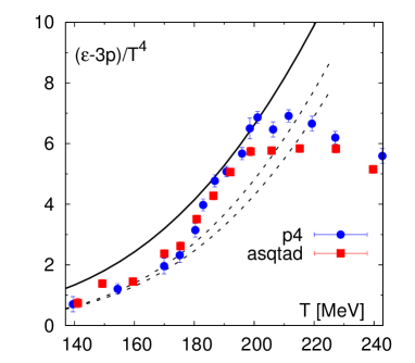
Figure 3: (Color online) The trace anomaly calculated in lattice QCD with p4 and asqtad actions on $N_{\tau}=6$ and 8 lattices compared with various parametrizations given by the solid, dotted and dashed lines (top) and the trace anomaly calculated in lattice QCD compared with the HRG model given by the solid and dashed lines (bottom). The figures are taken from Ref. Huovinen:2009yb .

Usual lQCD calculations for the thermodynamical variables assume that the system has infinite extent (volume $V\rightarrow\infty$) and it is homogeneous Boyd:1996bx . All thermodynamic quantities can be derived from the partition function Z($T,V$). The energy density and pressure are derivatives of the partition function with respect to $T$ and $V$ respectively

$$\epsilon = \frac{T^{2}}{V}\frac{\partial}{\partial T}lnZ\left(T,V\right),$$ (150)

$$P = T\frac{\partial}{\partial V}lnZ\left(T,V\right).$$ (151)

The pressure for a homogeneous system of infinite extent can be simply expressed in terms of $f$ as

$$P=\frac{T}{V}lnZ\left(T,V\right).$$ (152)

Using the above relations one can arrive at the following relationships

$$\epsilon =T\frac{\partial P}{\partial T}-P,$$ (153)

$$\Theta(T) =T\frac{\partial}{\partial T}\left(\frac{P}{T^{4}}\right),$$ (154)

where the trace anomaly, $\Theta(T)=(\epsilon-3P)/T^{4}$.

In the high temperature, $\Theta(T)$ can be reliably calculated from lQCD. On the other hand, at lower temperature the lQCD results are affected by possibly large discretisation effect. Therefore the usual practice to construct realistic EoS is to use the lattice data for the trace anomaly in the high temperature region ($T>250MeV$), and use HRG model in the low temperature region ($T<180MeV$). In the intermediate temperature $\Theta(T)$ is obtained by joining the parametrised high temperature and low temperature values smoothly (continuous first and second derivative). Once $\Theta(T)$ is known, pressure can be calculated by using Eq. (154). The energy density then can be readily obtained from Eq. (153). The top panel of Fig. 3 shows the trace anomaly calculated in lattice QCD with p4 and asqtad actions on $N_{\tau}=6$ and 8 lattices Bazavov:2009zn compared with various parametrizations given by the solid, dotted and dashed lines Huovinen:2009yb . The bottom panel shows the trace anomaly calculated in lattice QCD compared with the HRG model given by the solid and dashed lines Huovinen:2009yb .

VI Freeze-out: Spectra and Flow

In the late stage of hydrodynamics evolution of hot and dense nuclear matter created in high energy heavy-ion collisions, the density and the temperature reaches a critical value when the constituents no longer collides among themselves and thereafter they move in a straight trajectory towards the detectors. This phenomenon is known as freeze-out, more precisely the kinetic freeze-out. There is another chemical freeze-out when the particle number changing processes ceases. The chemical freeze-out temperature so far known to be higher than the kinetic freeze-out temperature.

In relativistic hydrodynamics simulations one also needs to stop the hydrodynamics evolution when the system reaches the kinetic freeze-out criterion. For this one needs to impose some physical constraints to calculate the freeze-out hyper-surface. This can be done by more than one way, we discuss here only the most popular choices used to calculate the freeze-out hyper-surface namely (i) the constant temperature freeze-out (ii) the constant energy density freeze-out (iii) the dynamical freeze-out. Among the three choices, the first two are based on the general idea that the pion (or other hadron) cross section is very sensitive to the temperature/energy density of the system, thus within short interval of temperature/energy density the condition for kinetic freeze-out is achieved. For the computational purpose this is realised by choosing a constant temperature/energy density surface.

The dynamical freeze-out is based on the idea that the ratio of expansion rate ($\theta$) to the collision rate ($\Gamma$) should be much much less than unity ($\frac{\theta}{\Gamma}\ll$ 1) in order to maintain the local thermal equilibrium essential for the applicability of the hydrodynamics evolution. One can then define the freeze-out criterion based on some predefined value of $\frac{\theta}{\Gamma}$ smaller than 1. Though the idea of dynamical freeze-out sounds more realistic it is not easy to implement in numerical calculation see Ref. Huovinen:2009yb for details.

The thermodynamical quantities of the fluid such as energy density, pressure and the fluid velocity obtained from the hydrodynamics simulation on the freeze-out surface are used to evaluate momentum distributions of the identified hadrons. The conversion of fluid to hadrons is done by using the Cooper-Frye procedure, see Ref. Cooper:1974mv for details. In Cooper-Frye procedure the momentum distribution (or invariant yield) of hadrons are calculated as Cooper:1974mv

$$E\frac{d^{3}N}{d^{3}p}=\frac{d^{3}N}{d^{2}p_{T}dy}=\int_{\Sigma}{f\left(x,p\right){p}^{\mu}d{\Sigma}_{\mu}},$$ (155)

where E, N, and $p^{\mu}$ are energy, number and four-momentum of hadrons, $d\Sigma_{\mu}$ is the differential freeze-out hyper-surface element. The distribution function, $f(x,p)$, consists of an equilibrium part, $f_{0}(x,p)$, and dissipative corrections, $\delta f(x,p)$. While the equilibrium distribution corresponding to the local thermodynamic quantities, as given in Eq. (105), is taken to be either Bose-Einstein or Fermi-Dirac distribution depending on the spin of the hadronic species, the dissipative correction is not unique, and will be explained in the following.

In the simple case when the dissipation is only due to the shear viscosity, leading-order moment method, also known as the Grad’s 14-moment approximation, leads to the well-known form of the viscous correction Grad ; Israel:1979wp

$$\delta f(x,p)=\frac{f_{0}\tilde{f}_{0}}{2(\epsilon+P)T^{2}}\,p^{\alpha}p^{\beta}\pi_{\alpha\beta},$$ (156)

where $\tilde{f}_{0}\equiv 1-rf_{0}$, with $r=1,-1,0$ for Fermi, Bose, and Boltzmann gases, respectively. Note that the viscous correction in this case increases with quadratic power of momenta. On the other hand, the Chapman-Enskog like iterative solution of the Boltzmann equation, Eq. (113), leads to a viscous correction which is effectively linear in momenta Bhalerao:2013pza ,

$$\delta f(x,p)=\frac{5f_{0}\tilde{f}_{0}}{2(\epsilon+P)T}\frac{1}{(u\cdot p)}\,p^{\alpha}p^{\beta}\pi_{\alpha\beta}.$$ (157)

It has been shown that, in contrast to Eq. (156) obtained using moment method, Eq. (157) leads to phenomenologically consistent corrections to the equilibrium distribution function, and is therefore a better alternative for hydrodynamic modeling of relativistic heavy-ion collisions Bhalerao:2013pza .

We note here that the calculation of four-dimensional freeze-out hyper-surface and the numerical evaluation of it is not trivial, for example see Ref. Huovinen:2012is for more details. Once we know the invariant momentum distribution the “n-th” order Fourier coefficient the flow harmonics $v_{n}$ can be readily obtained as

$$v_{n}=\frac{\displaystyle{\int_{y}dy\int_{p_{T}}d^{2}p_{T}\frac{d^{3}N}{d^{2}p_{T}dy}\cos\left[n\left(\phi_{n}-\psi_{n}\right)\right]}}{\displaystyle{\int_{y}dy\int_{p_{T}}d^{2}p_{T}\frac{d^{3}N}{d^{2}p_{T}dy}}}\,.$$ (158)

These above mentioned quantities are directly compared to the corresponding experimental data in order to obtain information about the transport coefficients such as shear and bulk viscosity of the QGP.

VII Resonance decay and hadronic rescattering

In high energy nuclear collisions various hadronic resonances are formed. The life time of most of the resonance particles are of the order of the expansion life time of the nuclear matter. The end product for the most of the decay channels involve pions. The decay of hadron resonances to pion enhances the pion yield specially at low transverse momentum, $p_{T}$. One can use the formalism given in Sollfrank:1990qz to calculate the relative contribution of the resonance decay to thermal pion spectra. The relative contribution of the resonance decay to pion spectra is a function of both the freeze-out temperature, $T_{\rm fo}$, and $p_{T}$. Thus the final $p_{T}$ spectra of $\pi$ are obtained by adding the contribution from resonance decay to the thermal $p_{T}$ spectra calculated from Cooper-Frye formula. The most dominant hadronic decay channels contributing to pion yield are: $\rho^{\pm}\rightarrow\pi^{\pm}\pi^{0},~{}\rho^{0}\rightarrow\pi^{-}\pi^{+},~{}K^{*\pm}\rightarrow\pi^{\pm}K^{0},~{}K^{*0}\rightarrow\pi^{-}K^{+},~{}\Delta\rightarrow\pi^{\pm,0}N,~{}\omega\rightarrow\pi^{+}\pi^{-}\pi^{0},~{}\eta\rightarrow\pi^{+}\pi^{-}\pi^{0}$, which should be considered with their corresponding branching ratios Sollfrank:1990qz .

According to the formalism given in Sollfrank:1990qz , to calculate the pion contribution from resonances, one need to provide the source temperature. The parametric fit to the ratio of the total pion to the thermal pion for the calculation at two different freeze-out temperature $T_{\rm fo}=130$ MeV and $150$ MeV are approximately given by Victor:thesis

$$\left.{\frac{\pi^{\pm}_{\rm total}}{\pi^{\pm}_{\rm thermal}}}\right|_{\rm T_{fo}=130MeV} =1.0121+\frac{1.4028}{1+\left(\displaystyle{\frac{\frac{p_{T}}{m_{\pi}}-0.0964}{3.666}}\right)^{\!2}}\,,$$ (159)

$$\left.{\frac{\pi^{\pm}_{\rm total}}{\pi^{\pm}_{\rm thermal}}}\right|_{\rm T_{fo}=150MeV} =1.0252+\frac{3.0495}{1+\left(\displaystyle{\frac{\frac{p_{T}}{m_{\pi}}-0.2302}{2.792}}\right)^{\!2}}\,,$$ (160)

where $m_{\pi}=139$ MeV is the pion mass. Note that about $\sim 50\%$ of the total pion yield come from resonance decay at LHC energy ($\sqrt{s_{NN}}=2.76$ TeV), whereas for RHIC energy ($\sqrt{s_{NN}}=200$ GeV) the resonance contribution to total pion yield is $\sim 30\%$ for $T_{\rm fo}=130$ MeV.

The sudden conversion of fluid to non-interacting hadrons at the freeze-out hyper-surface in the fluid dynamical evolution is hard to happen in practice. In reality the hydrodynamical picture should work fine for the early hot and dense phase of the QGP evolution when the scattering rate is comparatively large compared to the expansion rate. As the system grows in size and cools down with time the scattering rate goes down compared to the expansion rate. At some point of space-time, particularly in the late hadronic phase it is expected that the dynamical evolution most probably be governed by the microscopic Boltzmann equations considering multiple hadronic species and their collisions rather than the simplified macroscopic hydrodynamics evolution. Thus a complete dynamical evolution of high energy heavy-ion collisions contains simpler hydrodynamics evolution in the early time and a much computational expensive hadronic transport evolution in the late stage with the additional complexity of transforming fluid variables to position and momentum of hadrons.

For the hadronic rescattering phase several microscopic algorithms that solve coupled Boltzmann equations for a hadronic gas were developed in the 1980s and 1990s Aichelin:1986wa ; Stoecker:1986ci ; Sorge:1989dy ; Ehehalt:1996uq ; Zhang:1999bd ; Bass:1998ca ; Bleicher:1999xi . Hybrid codes that coupled an ideal fluid dynamical description of an expanding QGP to hadronic rescattering codes and compared the results with purely fluid dynamical calculations began to appear around 2000 Bass:2000ib ; Teaney:2001gc ; Hirano:2005xf ; Nonaka:2006yn . One of the first numerical code VISHNU that couples (2+1)D viscous hydro with a late hadronic Boltzmann cascade appeared in 2011 Song:2010aq . The use of these more sophisticated hybrid models are believed to reduce the uncertainty in the extracted value of $\eta/s$ of QGP, since the late hadronic stage is known to have larger shear viscosity which in usual viscous hydrodynamics simulations is not taken into account properly. We shall not go into the details of the hadronic transport model nor to the technical details of various techniques and uncertainties arising due to the matching of viscous hydrodynamics to the hadronic transport, details of which can be found in Ref. Song:2010aq and references therein. Before finishing this section we should point out one of the major findings of Ref. Song:2010aq , the $\eta/s$ of hadronic matter is found to be quite sensitive to the details of preceding hydrodynamics phase and on the switching temperature when the viscous hydrodynamics is switched to the hadronic transport evolution. The effort to better constraint the $\eta/s$ of QGP by using such sophisticated numerical models is a topic of current ongoing research.

VIII Transport coefficients

Determination of transport coefficients of the hot and dense QCD matter is one of the primary goal of theoretical simulations of relativistic heavy-ion collisions; see Heinz:2013th for a recent review. Ideal hydrodynamics has been proved to be quite successfully in the past to describe the spectra of produced particles in relativistic heavy-ion collisions. The presence of dissipation leads to dissipative entropy generation via Eq. (II.4.5), which results in the increase of total particle multiplicity for a fixed initial entropy. Shear viscosity, in particular, also leads to stronger radial flow leading to an increase in the mean transverse momentum of particles. However, the most important effect of shear viscosity is to suppress the elliptic flow coefficient, $v_{2}$, defined in Eq. (158) strongly. Therefore, in order to estimate the viscosity of the QCD matter within a hydrodynamic simulation, one has to tune the value of the specific shear viscosity, $\eta/s$, in order to fit the experimental data for $v_{2}$. One of the first estimates of $\eta/s$ was made within a hydrodynamics inspired blast-wave model Teaney:2003kp . Since then there has been a lot of activity in this field, which is briefly reviewed in the following.

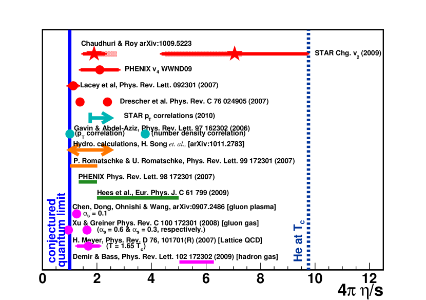
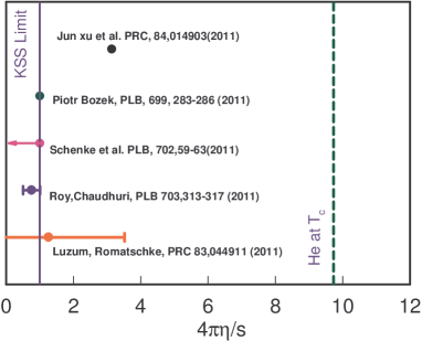
Figure 4: (Color online) Extracted values of $\eta/s$ for Au-Au collision at $\sqrt{s_{NN}}=200$ GeV (top) and for Pb-Pb collision at $\sqrt{s_{NN}}=2.76$ TeV (bottom) by different model calculations using different experimental observables. The solid vertical line at the left shows the lower limit of $\eta/s$ in unit of $1/(4\pi)$ Kovtun:2004de . For comparison we have also shown the $\eta/s$ of He at $T_{c}$ (dashed vertical line on the right).

Figure 4 (top panel) shows the extracted values of $\eta/s$ in different model calculations for Au-Au collisions at $\sqrt{s_{NN}}=200$ GeV Romatschke:2007mq ; Song:2010mg ; Chaudhuri:2010hr ; Lacey:2006bc ; Drescher:2007cd ; Gavin:2006xd ; vanHees:2008gj ; Chen:2009sm ; Xu:2007ns ; Meyer:2007ic ; Demir:2008tr . Most of the estimates are obtained by comparing experimental data for elliptic flow with model calculations. Some of the estimates used $p_{T}$ correlations and heavy meson $v_{2}$ data. The theoretical calculations include simulations with transport based approach as well as (2+1)D and (3+1)D viscous hydrodynamics with various initial conditions. Also shown are the results from lattice QCD calculation. All these results indicate that the $\eta/s$ value of the QGP fluid produced at top RHIC energies lies within $1-5\times 1/4\pi$ and is below the $\eta/s$ value of helium (blue dashed line) at $T_{c}$. The spread in the estimated values of $\eta/s$ reflects the current uncertainties associated with the theoretical calculations.

Figure 4 (bottom panel) shows $\eta/s$ estimated in various model calculations for Pb-Pb collision at $\sqrt{s_{NN}}=2.76$ TeV Xu:2011fe ; Bozek:2011wa ; Schenke:2011tv ; Luzum:2008cw . All the model calculations indicates that the values of $\eta/s$ of the QCD matter formed in heavy-ion collision at LHC lies between 1-4 $\times(1/4\pi)$. The specific shear viscosity was obtained in reference Xu:2011fe by using A Multi Phase Transport model (AMPT). Bozek Bozek:2011wa has estimated the specific shear viscosity of the fluid for LHC energy by using a (2+1)D viscous hydrodynamics model. In addition to shear viscosity, bulk viscosity ($\zeta/s=0.04$) in the hadronic phase was considered. Freeze-out and resonance decay was based on THERMINATOR event generator Kisiel:2005hn . Experimental data are best fitted with $\eta/s\sim 0.08$. A (3+1)D viscous hydrodynamics calculation with fluctuating initial conditions was done by Schenke et al. Schenke:2011tv . They explain the $v_{2}(p_{T})$ and $p_{T}$ integrated $v_{2}$ for different centralities. Their calculation shows that the experimental data measured at LHC by the ALICE collaboration are best described for $\eta/s$ value 0.08 or smaller. Luzum et al. Luzum:2008cw have estimated $\eta/s$ by using a (2+1)D viscous hydrodynamics simulation with smooth initial conditions for LHC energy to be same as at RHIC, $\eta/s=0.1\pm 0.1({\rm theory})\pm 0.08({\rm experiment})$. Comparison of experimentally measured integrated and differential $v_{2}$, the charged hadron $p_{T}$ spectra and multiplicity in the mid-rapidity and their global fit by minimising $\chi^{2}$ was done in Ref. Roy:2011xt by using a (2+1)D viscous hydrodynamics simulation, the extracted value of $\eta/s$ is $\sim 0.07\pm 0.01$.

The effects of bulk viscosity in hydrodynamic simulations of relativistic heavy-ion collisions have not been investigated as thoroughly as that of shear viscosity. In principle, the bulk viscosity of the QCD matter should not be zero for the range of temperatures achieved at the RHIC and the LHC, and it may become large enough to significantly affect the evolution of the medium Meyer:2007dy ; Paech:2006st . There has been several simulations of heavy-ion collisions that include the effect of bulk viscosity where it has been demonstrated that bulk viscosity can have a non-negligible effect on heavy-ion observables Ryu:2015vwa ; Noronha-Hostler:2013gga ; Song:2009rh ; Roy:2011pk ; Noronha-Hostler:2014dqa ; Denicol:2009am . However, there are various uncertainties in the extraction of bulk viscosity from the anisotropic flow data of heavy-ion collisions. For example, the theoretical uncertainties arising due to the ambiguities in the form of the specific bulk viscosity, $\zeta/s$, its relaxation time and the bulk viscous corrections to the freeze-out process, makes it difficult to study the effect of bulk viscosity on the evolution of QCD matter. Unlike shear viscosity, the extraction of bulk viscosity from hydrodynamic simulations is still unresolved and is currently an active research area.

IX Recent developments

IX.1 Flow in small systems: proton-proton and proton-nucleus collisions

As mentioned in the introduction, among the recent developments in the field of high energy heavy-ion collisions the most striking observation is the existence of radial flow like pattern in high multiplicity proton-proton (p-p) and proton-lead (p-Pb)collisions, for example see Ref. Loizides:2016tew for a summary of recent experimental results. At this point it needs some explanation why the observation of flow in small system is remarkable. One of the fundamental assumption when applying hydrodynamics to high energy nuclear collisions is that the system reaches a state of ”local thermal equilibrium” very quickly because of the strong interactions among the quarks and gluons. In heavy-ion collisions such as Pb-Pb or Au-Au the number of participating nucleons are large, for example for a head-on Au-Au or Pb-Pb collisions there are 197+197 and 208+208 participating nucleons. Each of these colliding nucleons on average produce more than one particles in each collisions, thus the total number of degrees of freedom in the system created just after the collisions are large. They collide among themselves through strong interaction and subsequently reaches local thermal equilibrium (we note here that the full mechanism by which the system reaches local thermal equilibrium within such a short period of time is not fully understood yet).

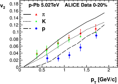
Figure 5: (Color online) Elliptic flow, $v_{2}$, of identified particles from the hydrodynamic model compared to the ALICE data ABELEV:2013wsa . The figure is taken from Ref. Bozek:2014wpa .

The situation is very different in smaller colliding systems such as p-p or p-Pb where the number of participating nucleons and the numbers of produced particles are comparatively smaller in numbers. It is very counterintuitive that with such few number of particles the system reaches local thermal equilibrium within a very short time-period. On the other hand, event generators based on perturbative QCD such as PYTHIA and HIJING have successfully described various observables associated with particle production in p-p collisions. Thus p-p as well as p-nucleus collisions have been for long time considered qualitatively different from heavy-ion collisions, for which the hydrodynamic description became a mainstream since its successful explanation of RHIC data. It is interesting to note that the p-p collisions were used as a benchmark for studying the existence of QGP in larger systems where a thermalised medium is believed to be created.

This situation changed recently as the CMS and ATLAS collaboration observed a “ridge” like correlation in the azimuthal distribution of charged hadrons produced in high multiplicity p-p or p-Pb collisions. In those experiments a mass dependence of the slope of identified hadron’s $m_{T}$ spectrum in high multiplicity p-Pb and p-p collisions were also observed. All these phenomenon are known to be the most significant indication for existence of hydrodynamic flow in larger colliding systems such as Au-Au or Pb-Pb. Like in heavy-ion collisions, the PYTHIA model failed to describe these observed experimental measurement for high multiplicity p-p or p-Pb events unless it employs some special mechanism like Color Reconnection (CR) and Multi Parton Interaction (MPI) with an additional free parameter to explain the experimental data Ortiz:2013yxa . On the other hand, the relativistic hydrodynamic models with large radial velocity have been proved to be quite successful in describing the same experimental data. It is also worthwhile to mention that there are some other theoretical conjectures about these recent observation which does not incorporate this hydrodynamics like flow, but till now those studies lack detailed numerical calculation in order to compare it with the experimental data Ref. Gyulassy:2014cfa .

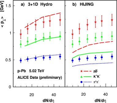
Figure 6: (Color online) Average transverse momentum of identified particles in p-Pb collisions at $\sqrt{s_{NN}}$=5.02 TeV, the experimental data (various symbols) from ALICE Collaboration ABELEV:2013wsa , compared to the results of the HIJING model and of the viscous hydrodynamics. The figure is taken from Ref. Bozek:2014wpa .

• p-Pb collisions: Recent experimental measurement shows that the number of charged particle produced in p-Pb collisions at $\sqrt{s_{NN}}=5.02$ TeV is similar to those in peripheral Pb-Pb collisions Ref. Chatrchyan:2013nka . Considering the fact that final charged multiplicity is proportional to the initial energy/entropy density it is clear that the initial energy density in most violent p-Pb collisions is similar as in heavy-ion collisions. In fact the collision zone in p-Pb collisions is expected to be smaller than the peripheral Pb-Pb collisions, consequently the energy density is higher in high multiplicity p-Pb events than the peripheral Pb-Pb events. The initial high energy density within small volume in p-Pb collisions creates favourable condition for the subsequent hydrodynamics evolution. Another strong evidence of hydrodynamical flow in p-Pb collisions came from the observation of mass dependence of slope of identified hadrons $p_{T}$ spectra, measured in experiment Ref. Chatrchyan:2013eya . The experimentally measured $v_{n}$ and $v_{2}(p_{T})$ data for identified hadrons in p-Pb collisions by CMS Chatrchyan:2013nka and ALICE ABELEV:2013wsa collaboration is nicely explained by a (3+1)D viscous hydrodynamics model study by Bozek et al. in Ref. Bozek:2014wpa (see Fig. 5). In addition to that the mean transverse momentum of identified hadrons is also explained within the same (3+1)D hydrodynamic model, whereas, the Monte-Carlo event generator model HIJING which is based on the perturbative QCD processes relevant to the collisions fails to explain the same experimental data as can be seen in Fig. 6. This already gives the indication that for the high multiplicity p-Pb collisions QGP is produced and it flows like fluid before freezing out to hadrons.

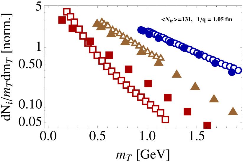
Figure 7: (Color online) Normalized spectra of pions (squares), kaons (triangles) and protons (discs) for p-p collisions. Open symbols correspond to the CMS data Chatrchyan:2012qb for $|\eta|<2.4$ and $\sqrt{s}=7$ TeV, while the solid ones are obtained from the best one-parameter fit of the Gubser’s flow. The figure is taken from Ref. Kalaydzhyan:2015xba .

• p-p collisions: Qualitatively similar signature of collective behaviour is also observed in high multiplicity p-p collisions like high multiplicity p-Pb collisions. However, the initial measurement shows that the $p_{T}$ integrated $v_{2}$ and $v_{3}$ is 30% and 50% smaller than in p-Pb at similar multiplicity. Like heavy-ion and p-Pb collisions a simple hydrodynamic inspired model with large radial velocity has successfully explained the experimental observation of mass dependence of slope in p-p collisions; see Fig. 7 which is taken from Ref. Kalaydzhyan:2015xba . In a similar effort a blast wave model fit was shown to be inconsistent with the experimental data, see Ref. Ghosh:2014eqa for details. There are some studies of viscous hydrodynamics for p-p collisions for example see Ref. Bozek:2010pb ; Prasad:2009bx ; Bzdak:2013zma , more extensive study is needed for the comparison of all experimentally available data. We note here that it is still an open question whether the small system created in p-p collisions are big enough or live long enough for hydrodynamics to be applicable, detailed discussion of which is out of the scope of the present review. We refer to see the Ref.  Shuryak:2013ke for a detailed discussion about the applicability of hydrodynamics in small systems.

IX.2 Flow in ultra central collisions

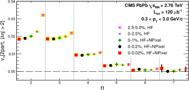
Figure 8: (Color online) Top panel: The $v_{n}$ (n=2-6) values as a function of $p_{T}$ in 0.0-0.2% central Pb+Pb collisions at $\sqrt{s_{NN}}=2.76$ TeV. Bottom panel: Experimental measurement of $p_{T}$-averaged (0.3-3.0 GeV) $v_{n}$ as a function of “n” in five centrality classes (2.5-5.0%, 0-2.5%, 0-1%, 0-0.2% and 0-0.02%) for Pb+Pb $\sqrt{s_{NN}}=2.76$ TeV collisions. Error bars denote the statistical uncertainties, while the shaded color boxes correspond to the systematic uncertainties. The data was measured by the CMS collaboration and the figures are taken from Ref. CMS:2013bza .

As mentioned earlier, the hydrodynamic response of the anisotropy in the initial overlap geometry in the configuration space transforms to the final momentum space anisotropy giving rise to non-zero values of flow harmonics $v_{n}$. The most prominent flow harmonics $v_{2}$ originates as a hydrodynamic expansion of the initial elliptic shape of the fireball. The conversion efficiency of the spatial deformation into the momentum space anisotropy is very sensitive to the shear viscosity over entropy density ($\eta/s$) and the initial configuration of the system. The extraction of $\eta/s$ of QGP by comparing hydrodynamic simulation results to the corresponding experimental data is riddled with large uncertainties in our understanding of the initial-state conditions of heavy-ion collisions. For example, viscous hydrodynamic simulation with MC-Glauber initial condition gives very different values of $\eta/s$ compared to the same simulation with different initial condition such as MC-KLN. This uncertainty due to the poorly known initial condition can be minimised in case of ultra central collisions. In ultra-central collisions $v_{2}$ and other higher flow harmonics solely originate from the initial fluctuating energy density since the overlap zone in ultra central collisions are almost circular.

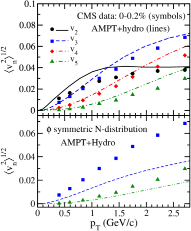
Figure 9: (Color online) Comparison of a (2+1)D viscous hydrodynamics simulation with the initial condition from AMPT model to corresponding experimental data for root mean squared values of $v_{n}$ for $n=2-5$; figure is from Ref. Bhalerao:2015iya .

For ultra central collisions the initial collision geometry is predominantly generated by fluctuations such that various orders of eccentricities predicted by different models tend to converge. Therefore, studies of $v_{n}$ in ultra-central heavy-ion collisions can help to reduce the systematic uncertainties of initial-state modelling in extracting the $\eta/s$ value of the system. Let us first discuss the recent experimental results for ultra central Pb-Pb collisions at LHC, after that we shall also discuss the corresponding results from viscous hydrodynamics simulations. Top panel of Fig. 8 shows the experimentally measured differential flow coefficients $v_{n}$ as a function of $p_{T}$ for 0-0.2% centrality Pb-Pb collisions at $\sqrt{s_{NN}}=2.76$ TeV. The $v_{n}$’s were calculated using 2 particle correlation method with large pseudo-rapidity gap $|\Delta\eta|>2$ between the two hadrons. The bottom panel of Fig. 8 shows the $p_{T}$ integrated $v_{n}$ (n=2-7) in ultra central Pb-Pb collisions for five different collisions centrality. The experimental data and the figure are taken from Ref. CMS:2013bza . Before we proceed any further we note the following experimental observation from the CMS paper.

• At higher transverse momentum ($p_{T}\geq\ 2$ GeV), $v_{2}$ becomes even smaller than the higher-order $v_{3},v_{4}$, and at much higher values of $p_{T}$ it becomes smaller than other higher order $v_{n}$.

• The $p_{T}$ averaged $v_{2}$ and $v_{3}$ are found to be equal within 2%, while other higher-order $v_{n}$ decrease as n increases.

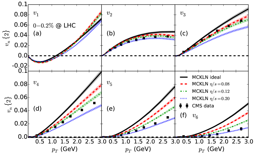
Figure 10: (Color online) Comparison of $p_{T}$ dependent $v_{n}\left\{2\right\}$ of charged hadrons in $2.76$ A TeV Pb+Pb collisions at 0-0.2% centrality for viscous hydrodynamics simulations (various lines) with the corresponding experimental results (solid squares); the figure is from Ref. Shen:2015qta .

The evolution of the QGP according to relativistic hydrodynamics simulations have been able to consistently explain experimentally measured $v_{n}$’s for different centralities and for different colliding energies, it is natural to expect that it should also explain the measured $v_{n}$ in the ultra central collisions. Before we discuss the results of hydrodynamic simulations, we note that one need to carefully select events into centrality classes since the integrated $v_{n}$’s are quite sensitive on the selection of centrality class as can be seen from the bottom panel of Fig. 8. We also note that it is computationally expensive to simulate such ultra-central collisions since the number of events within the given centrality class is significantly small compared to the total number of minimum bias events. Although the essential $p_{T}$ dependence of charged hadrons $v_{n}$ and their observed ordering for ultra-central Pb-Pb collisions was nicely explained by a viscous hydrodynamic simulation using initial conditions from AMPT model Bhalerao:2015iya ; see Fig. 9. However on careful observation we notice that at low $p_{T}<1.5$ GeV, the splitting from hydrodynamics simulation is larger than the corresponding experimental measurement. Similar disagreements are also evident for $p_{T}>1.5$ GeV in Fig. 10, which is taken from Ref. Shen:2015qta . This can be seen more clearly from the $p_{T}$ integrated $v_{2}$ and $v_{3}$ in Fig. 11 which is also taken from Ref. Shen:2015qta . In Ref. Shen:2015qta , the $p_{T}$ integrated $v_{n}$ was studied using (2+1)D viscous hydrodynamics model with MC-Glauber and MC-KLN initial conditions.

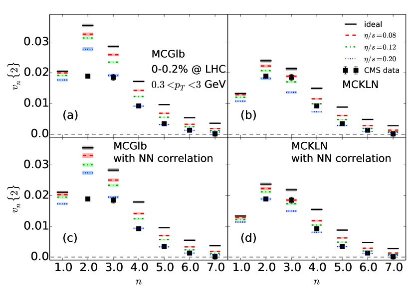
Figure 11: (Color online) Comparison of $p_{T}$ integrated $v_{n}\left\{2\right\}$ of charged hadrons in $2.76$ A TeV Pb+Pb collisions at 0-0.2% centrality for viscous hydrodynamics simulations (various lines) with the corresponding experimental results (solid squares). Plot (a) and (c) are are for MC-Glauber initial conditions, and (b),(d) corresponds to MC-KLN initial conditions. Results in the top two panels (a) and (b) was obtained by considering nucleons with a repulsive hard core, whereas the results in the bottom panel (c) and (d) are obtained for the initial conditions with finite nucleon-nucleon correlations. The figure is taken from Ref. Shen:2015qta .

The nucleon-nucleon correlations in the colliding nucleus were also considered as a potential cause behind the experimentally measured $v_{2}\sim v_{3}$. However, none of the initial condition model has so far been able to simultaneously explain the experimentally measured $v_{n}$’s, as can be seen in Figs. 9, 10 and 11. In this regard we note that Denicol et al., Ref. Denicol:talk_ECT , have considered bulk viscosity along with the shear viscosity and the nucleon-nucleon correlations in order to explain this apparent discrepancy between the experimental data and corresponding theoretical results, although there was some improvement but so far the effort remains unfruitful.

IX.3 Longitudinal fluctuations and correlations

In relativistic heavy-ion collision experiments, a fraction of the incoming kinetic energy is converted into new matter deposited in the collision zone. The distribution of this matter in the plane transverse to the colliding beams is inhomogeneous and fluctuates from collision to collision. The lumpy initial energy density distribution and its event-by-event fluctuations lead to anisotropic flows of final hadrons through collective expansion in high energy heavy-ion collisions. The first numerical demonstration of the role of lumpy initial energy density (or event-by-event fluctuation) in the transverse plane (plane defined by the impact parameter vector and one of the perpendicular axis to the beam direction) to the experimentally observed non-zero odd flow harmonics (particularly third harmonics $v_{3}$) in heavy-ion collision was made by Alver and Roland Alver:2010gr . From then on experimentally measured flow harmonics for all order (even and odd) has been successfully explained by viscous hydrodynamics model studies with fluctuating initial conditions such as Monte-Carlo (from now on we denote it by MC) GlauberBroniowski:2007ft ; Hirano:2009ah , MC-CGC Roy:2012pn , URQMD Petersen:2008dd , EPOS Werner:2010aa , AMPT Pang:2012he , and IP-Glasma Schenke:2012wb . Fluctuations in the transverse plane not only give rise to odd flow harmonics but also significant even and odd $v_{n}$ in ultra central collisions Ma:2010dv . They also result in $p_{T}$ dependent event planes, which break down the flow factorization $v_{n,n}(p_{T1},p_{T2})=v_{n}(p_{T1})v_{n}(p_{T2})$ Aamodt:2011by . Like the lumpy initial energy density in the transverse plane, it is also expected (the reason for which will be discussed shortly) that the energy density is lumpy in the longitudinal (space rapidity) direction.

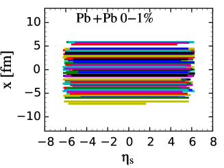
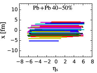
Figure 12: (Color online) Distribution of strings created between the partons of two colliding Pb nucleus as a function of space-time rapidity ($\eta_{s}$) at $\sqrt{s_{NN}}=2.76$ TeV for $0-1$% (top panel) and 40-50% (bottom panel) collision centrality. The figure is taken from Ref. Pang:2015zrq .

Recent measurement of decorrelation of anisotropic flow along longitudinal direction by CMS collaboration has corroborated the above expectation. Studies of fluctuations along the longitudinal direction and their effects on anisotropic flows of final charged hadrons have only recently been started. At present the current understanding of longitudinal correlation (or decorrelation) of flow harmonics is as follows

• The fluctuations of energy density along the longitudinal direction due to the fragmentation and different lengths of the coloured string produced in the scattering of nucleons Pang:2015zrq ; Pang:2014pxa ; Broniowski:2015oif .

• A gradual twist of the fireball (or more specifically the event plane) along the longitudinal direction Ref. Bozek:2010vz ; Jia:2014ysa .

Let us discuss each of them separately. Regarding the contribution of colour string we shall particularly discuss here a recent study Ref. Pang:2015zrq where AMPT transport model is used to evaluate the initial conditions for (3+1)D hydrodynamic model.

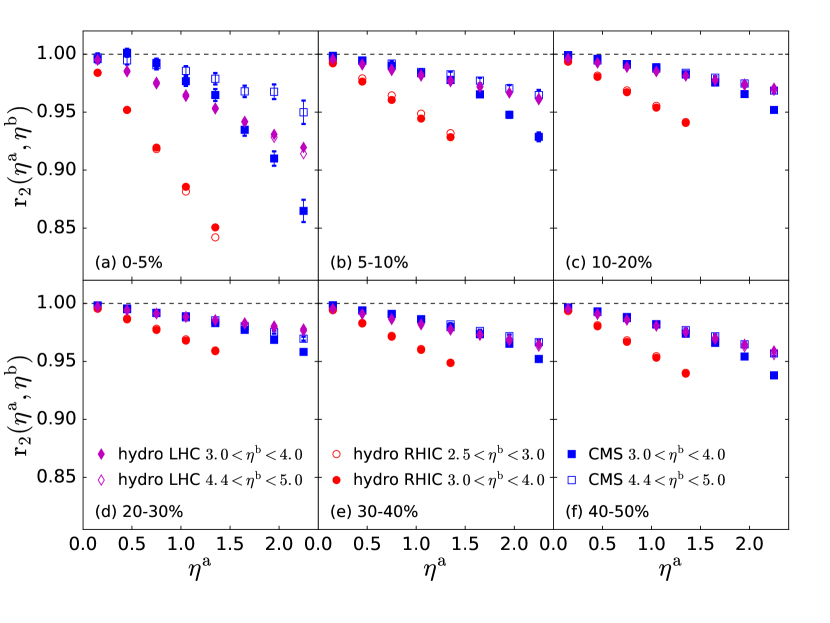
Figure 13: (Color online) Top panel: The factorization ratio $r_{2}$ as a function of space-time rapidity $\eta^{a}$ for two different reference rapidity bin $3.0<\eta^{b}<4.0$ and $4.4<\eta^{b}<5.0$ in Pb-Pb collisions at $\sqrt{s_{NN}}=2.76$ TeV (open and solid diamonds), and for $2.5<\eta^{b}<3.0$ and $3.0<\eta^{b}<4.0$ in Au-Au collisions at $\sqrt{s_{NN}}=200$ GeV (open and solid circles) from event-by-event (3+1)D ideal hydrodynamics simulations compared with experimental data from CMS collaboration Ref. Khachatryan:2015oea for Pb-Pb collisions at $\sqrt{s_{NN}}=2.76$ TeV (empty and solid squares). The figures are from Ref. Pang:2015zrq .

AMPT uses HIJING to generate initial partons from hard and semi-hard scatterings and excited strings from soft interactions. The number of mini-jet partons per binary nucleon-nucleon collision in hard and semi-hard scatterings follow a Poisson distribution with the mean value given by the jet cross-section. The number of excited strings is equal to the number of participant nucleons in each event. Besides random fluctuations from mini-jet partons, the parton density fluctuates along longitudinal direction according to the length of strings. There are basically three types of strings:

1. Strings associated with each wounded nucleon (between a valence quark and a diquark),

2. Single strings between q-q pairs from quark annihilation and gluon fusion processes,

3. Strings between one hard parton from parton scatterings and valence quark or diquark in wounded nucleons.

These strings finally fragment into the partons along the longitudinal direction and giving rise to fluctuating energy density distribution in $\eta_{s}$, see Fig. 12 for the distribution of coloured strings in the longitudinal direction for a typical Pb-Pb collision at $\sqrt{s_{NN}}=2.76$ TeV. For more details about the longitudinal fluctuations and the visualization of parton density distribution in $\eta_{s}$ see Ref. Pang:2015zrq .

The idea of a gradual twist of the fireball (or torqued fireball) along the longitudinal direction is due to Piotr Bozek et al. Bozek:2010vz . According to Bozek et al. the following ingredients are responsible for the appearance of the torque effect:

1. Statistical fluctuations of the transverse density of the sources (wounded nucleons), and

2. The asymmetric shape of the particle emission function, peaked in the forward (backward) rapidity for the forward (backward) moving wounded nucleons.

We note that in this model, the initial energy density profile is parametrized in such a way that after the hydrodynamics evolution and the freeze-out the hadronic spectra produced at different rapidities match with the corresponding experimental data. Whereas in the case of AMPT initial condition we do not need to use such procedure in order to explain the corresponding experimental data, for example in Fig. 13 we show the comparison of experimental data of longitudinal correlation for Pb-Pb collisions from CMS collaboration Khachatryan:2015oea and a (3+1)D hydrodynamics simulation result with AMPT initial condition. Note that with AMPT initial condition the experimental data is quite well described by the (3+1)D ideal hydrodynamics simulation. In the AMPT initial condition both longitudinal fluctuations and torque effects are present, the interplay of twist and fluctuation and the relative contribution of this two effects in heavy-ion collisions was studied within (3+1)D hydrodynamics model and AMPT in Ref. Pang:2014pxa .

Many techniques have been proposed to study the longitudinal structure of final hadron production in heavy-ion collisions and the underlying mechanisms. For example, three-particle correlations were suggested to measure the twist effect Borghini:2002hm in heavy-ion collisions at RHIC. One can also characterise the longitudinal fluctuations in terms of coefficients in the Chebyshev polynomials Bzdak:2012tp and the Legendre polynomial expansion of two-particle correlations in pseudorapidity Monnai:2015sca ; Bozek:2015tca . The most intuitive method is to measure the forward-backward (FB) event plane angles or anisotropic flow differences Pang:2014pxa with varying pseudorapidity gaps. These methods are used within the torqued fireball model Bozek:2010vz , (3+1)D hydrodynamics model and the AMPT model Pang:2014pxa ; Xiao:2012uw to study the decorrelation of event plane angles or anisotropic flow along the pseudorapidity direction. Jia et al. Jia:2014ysa also proposed an “event-shape twist” technique to study the event plane decorrelation due to the twist in initial energy density distributions by selecting events with big FB event plane angle differences. Alternatively by selecting events with vanishingly small FB event plane angle differences, one can then eliminate the twist effect and the measured decorrelation of anisotropic flow with finite pseudorapidity gaps should be caused only by random fluctuations of event plane angles as was done in Ref. Pang:2014pxa . Before ending this section we note that the experimentally observed difference in the longitudinal correlation ($r_{2}$ and $r_{3}$) for different reference rapidity bin Khachatryan:2015oea is not yet understood within theoretical model studies Pang:2015zrq . We need further studies in order to understand those finer details.

IX.4 Flow in intense magnetic field

The most strongest known magnetic field ($|\vec{B}|\sim 10^{18}-10^{19}$ Gauss) in the universe is produced in laboratory experiments of Au-Au or Pb-Pb collisions such as at RHIC and at LHC. Previous theoretical studies show that the intensity of the produced magnetic field rises approximately linearly with the centre of mass energy ($\sqrt{s_{{\rm NN}}}$) of the colliding nucleons Bzdak:2011yy ; Deng:2012pc . The corresponding electric fields in such collisions also becomes very strong which is same order of magnitude as the magnetic field ($e\vec{B}\approx e\vec{E}\sim 10m_{\pi}^{2}$ for a typical Au-Au collision at top RHIC energy $\sqrt{s_{\rm NN}}=200$ GeV) Bloczynski:2012en , where $m_{\pi}$ is the pion mass. Such intense electric and magnetic fields are strong enough to initiate the particle production from vacuum via Schwinger mechanism KEKIntense:2010 .

Figure 14: (Color online) Distribution of nucleons inside target and projectile nuclei in a typical Au-Au collision at $\sqrt{s_{\rm NN}}=200$ GeV for $b=12$ fm. Figure is from Ref. Roy:2015coa .

The origin of such large electric and magnetic field is the relativistic velocities of the positive charge nucleus. Within a MC Glauber model the electric ($\vec{E}$) and magnetic ($\vec{B}$) field at position $\vec{r}$ and at time $t$ for a nucleus of charge $Ze$ moving with velocity $\vec{v}$ in straight line is given by

$$\vec{E}\left(\vec{r},t\right) =\frac{e}{4\pi}\sum_{i=1}^{{N}_{proton}}{{Z}_{i}\frac{\vec{{R}_{i}}-{R}_{i}\vec{{v}_{i}}}{{\left({R}_{i}-\vec{{R}_{i}}\cdot\vec{{v}_{i}}\right)}^{3}}\left(1-{v}_{i}^{2}\right)},$$ (161)

$$\vec{B}\left(\vec{r},t\right) =\frac{e}{4\pi}\sum_{i=1}^{{N}_{proton}}{{Z}_{i}\frac{\vec{{v}_{i}}\times\vec{{R}_{i}}}{{\left({R}_{i}-\vec{{R}_{i}}\cdot\vec{{v}_{i}}\right)}^{3}}\left(1-{v}_{i}^{2}\right)}.$$ (162)

Here $\vec{R_{i}}=\vec{x}-\vec{x_{i}}(t)$ is the distance from a proton at position $\vec{x_{i}}$ to $\vec{x}$ where the field is evaluated. In the above expression the summation index $i$ denotes the contribution of all protons inside the colliding nucleus, for example Fig. 14 shows the positions of nucleons inside the two Au nucleus for a typical peripheral collision calculated in MC-Glauber model. Due to the fluctuating proton position from event to event the electric and magnetic field becomes irregular both in direction and in magnitude in the transverse plane. Moreover, the magnetic field in the central collisions becomes non-zero for such initial random proton positions. This can be seen from Fig. 15 where the event averaged value of $B_{y}$ as a function of impact parameter $b$ is shown. The black dashed-dotted line corresponds to the average of the absolute magnitude of $B_{y}$ which is clearly non-zero even for $b=0$ fm collisions. Note that we have used the natural unit where $\hbar=c=k_{b}=\varepsilon_{0}=\mu_{0}=1$, with this choice the electric charge $e=\sqrt{\frac{4\pi}{137}}$ becomes a dimensionless number. In the limit $v\sim c$, the denominator in Eq. (161) and (162) becomes very small and we have large $\vec{E}$ and $\vec{B}$.

There are large number of theoretical predictions based on the expectation of the creation of large magnetic field in heavy-ion collisions such as chiral magnetic effect, chiral electric effect, chiral magnetic waves etc., the discussion of which is beyond the scope of this review. For more details, we refer the reader to the following references Kharzeev:2013ffa ; Bzdak:2012ia ; Kharzeev:2015kna ; Tuchin:2014hza ; Huang:2015oca . Here we will concentrate on the possible effect of this large electro-magnetic field on the initial energy density and the subsequent hydrodynamics evolution of QGP produced in RHIC or LHC experiments. To the best of our knowledge, one of the first numerical study of the effect of magnetic fields on the hydrodynamics evolution in heavy-ion collisions are by Gursoy et al. Gursoy:2014aka and by Hirono et al. Hirono:2014oda . However, those studies were based on several assumptions and none of them have considered the full magneto-hydrodynamics solution for the QGP evolution. We note here that the electric and magnetic field might affect the initial energy density, subsequent hydrodynamics stage, and the freeze-out distribution functions provided that the field is strong enough and lives until freeze-out.

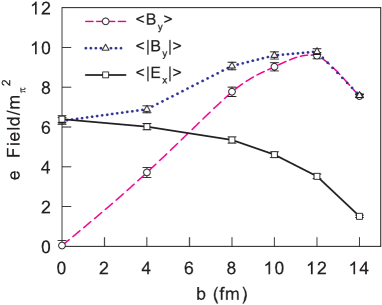
Figure 15: (Color online) Impact parameter dependence of event averaged magnetic and electric fields at the centre of the fireball for Au-Au collisions at $\sqrt{s_{\rm NN}}=200$ GeV. Figure is from Ref. Roy:2015coa .

One of us has recently studied the importance of electromagnetic field energy density compared to the energy density of the QGP fluid for Au-Au collisions at $\sqrt{s_{NN}}=200$ GeV in Ref. Roy:2015coa . The ratio ($\sigma$) of the magnetic field energy density to the fluid energy density was found to be $\sim 1$ for peripheral collisions, but in central collisions $\sigma<<1$. It was also found that electric field also contributes similar energy density as magnetic field. Recent study by Tuchin Tuchin:2013apa shows that the decay of the initial magnetic field can be substantially delayed in the case of finite electrical conductivity of QGP. Thus it becomes increasingly important to consider the electromagnetic field in the hydrodynamic evolution of heavy-ion collisions Tuchin:2013ie . In Refs. Roy:2015kma ; Pu:2016ayh ; Pu:2016bxy analytic solution of relativistic hydrodynamics for simplified cases was obtained. Finding analytic solution for general initial conditions is very difficult and there are very few analytical solution that exists for relativistic magnetohydrodynamics. The only possible way is to use numerical methods to solve magnetohydrodynamic equations relevant for heavy-ion collisions. This is not an easy task to accomplish. Initial effort in this direction can be found in Ref. Pang:2016yuh . However, we note that the authors of Ref. Pang:2016yuh have solved usual hydrodynamics conservation equations (without magnetic field) by considering an external force originating due to the paramagnetic interaction of QGP with the magnetic field.

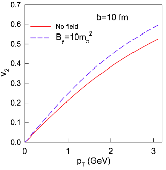
Figure 16: (Color online) Elliptic flow of $\pi^{-}$ as a function of $p_{T}$ for b=10 fm Au-Au collisions at $\sqrt{s_{\rm NN}}=200$ GeV. Red line corresponds to (2+1)D ideal hydrodynamics result without magnetic field, the blue dashed line correspond to $v_{2}$ with external magnetic field.

One of us has also recently solved the hydrodynamics equations where magnetic field is taken into account in the energy-momentum tensor of the fluid. A realistic space and time dependence of magnetic field is considered for an ideal fluid evolution in Au-Au collisions at $\sqrt{s_{NN}}=200$ GeV. It is found that in the presence of a finite electrical conductivity of QGP, the elliptic flow of $\pi^{-}$ increases noticeably, depending on the details of the magnitude of the magnetic field and the subsequent time evolution of the field. This is still a very new field of study and at present more detailed investigations are underway. In Fig. 16 we show the $v_{2}$ of $\pi^{-}$ obtained for impact parameter $b=10$ fm Au-Au collisions at $\sqrt{s_{NN}}=200$ GeV collisions. Initial value of magnetic field is taken to be $10m_{\pi}^{2}$ and the time variation of the magnetic field is obtained by parametrizing the results from Ref. Tuchin:2013apa . A realistic spatial profile for y-component of magnetic field was considered for the simulation. From Fig. 16 one can see that $v_{2}$ of $\pi^{-}$ is noticeably enhanced in the presence of magnetic field (blue dashed line) compared to the case of no magnetic field (red line).

X Outlook

In this review article, we have discussed various aspects of relativistic dissipative hydrodynamics and its application to high energy heavy-ion collisions. While considerable success has been achieved in explaining many experimental observations, there are several issues that still needs further investigation. For example the experimentally measured longitudinal correlation of flow harmonics shows a splitting in the quantities corresponds to the correlation measure namely $r_{2}\left(\eta_{a},\eta_{b}\right)$ and $r_{3}\left(\eta_{a},\eta_{b}\right)$ for two different reference rapidity windows, which cannot be explained within a (3+1)D ideal hydrodynamics model with initial condition obtained from HIJING model. The reason behind this experimentally observed difference in $r_{2}\left(\eta_{a},\eta_{b}\right)$ and $r_{3}\left(\eta_{a},\eta_{b}\right)$ is still poorly understood.

It was also argued in the present review that the effect of magnetic field might not be negligible on the hydrodynamics evolution of QGP produced in heavy-ion collisions. Particularly it may be important for the reason that the elliptic and higher-order flow harmonics might be affected under such strong magnetic field. However, at present there are some open issues in this regard: the electrical conductivity of the QGP might play an essential role in the temporal decay of the magnetic field. A poor knowledge of the temperature dependent electrical conductivity is one of the major source of uncertainties. In addition to that, the magnetic susceptibility of the QGP and the hadron resonance gas should be included for a realistic calculation.

Another unsolved problem is the experimentally measured $v_{2}$, $v_{3}$ in ultra-central collisions. Within error bars the magnitude of $v_{2}$ and $v_{3}$ are observed to be same for ultra-central collisions (0-0.2%). Although viscous hydrodynamics model with MC-KLN initial condition considering nucleon-nucleon correlations produces quite close result to the experimental measurement, it is still not fully explained within the given error. Another puzzling aspect of high energy collisions is the observation of flow like behaviour in small systems. Initial study shows that the experimentally observed flow harmonics and other bulk observables for high multiplicity p-p and p-Pb collisions can be well described within viscous hydrodynamics model simulation. A detailed theoretical explanation of how such small system behave collectively is still not well understood. There are also possibility for non-hydrodynamical origin of this observed flow in such small system. This is a topic of current research and we hope we will have more clear theoretical understanding within next few years when further studies including alternative possibilities will be available.

Finally we note that the field of high energy collisions is a very active area of research, we have not covered all aspects of the recent developments in the field related to hydrodynamics/collectivity of the QGP. For example the event-by-event distribution of flow harmonics Aad:2013xma and their correlations Bilandzic:2013kga ; ALICE:2016kpq emerges as a promising observable to better constrain the initial conditions and the shear viscosity of the QGP. The event-by-event study of photon and dilepton production within viscous hydrodynamics provide us another window to look at the early stages of the heavy-ion collisions Chatterjee:2014nta ; Shen:2014lpa . We hope that through all these ongoing experimental and theoretical/phenomenological studies we will have much refined understanding about the collective behaviour and the transport properties of the QGP in the near future.

Conflict of Interest

The authors declare that there is no conflict of interest regarding the publication of this article.