Modelling turbulent stellar convection zones: sub-grid scales effects

Abstract

The impressive development of global numerical simulations of turbulent stellar interiors unveiled a variety of possible differential rotation (solar or anti-solar), meridional circulation (single or multi-cellular), and dynamo states (stable large scale toroidal field or periodically reversing magnetic fields). Various numerical schemes, based on the so-called anelastic set of equations, were used to obtain these results. It appears today mandatory to assess their robustness with respect to the details of the numerics, and in particular to the treatment of turbulent sub-grid scales. We report on an ongoing comparison between two global models, the ASH and EULAG codes. In EULAG the sub-grid scales are treated implicitly by the numerical scheme, while in ASH their effect is generally modelled by using enhanced dissipation coefficients. We characterize the sub-grid scales effect in a turbulent convection simulation with EULAG. We assess their effect at each resolved scale with a detailed energy budget. We derive equivalent eddy-diffusion coefficients and use the derived diffusivities in twin ASH numerical simulations. We find a good agreement between the large-scale flows developing in the two codes in the hydrodynamic regime, which encourages further investigation in the magnetohydrodynamic regime for various dynamo solutions.

1 Introduction

Cool stars are known to possess a substantial convection zone forming their outer layer. The convective motions participate in the self-organization of the interior of the star and in particular in the sustainment of a large scale differential rotation (e.g. Brun and Toomre 2002; Featherstone and Miesch 2015, and references therein), and a potentially cyclic magnetism (e.g. Ghizaru et al. 2010; Käpylä et al. 2012; Augustson et al. 2015; Brun et al. 2015, and references therein). Understanding the properties of solar and stellar convection is hence of prior importance to understand the joint evolution of the stellar rotation rate and large-scale magnetic fields along the Main Sequence.

Thanks to helioseismology (Christensen-Dalsgaard et al. 1991; Basu 1997), we know that the solar stratification is close to adiabatic down to 0.71 solar radii, leaving little doubt that convective motions extend down to such depths. However, the amplitude of these deep convective flows in the Sun is today the subject of a stimulating controversy. Using time-distance helioseismology, Hanasoge et al. (2010, 2012) obtained surprisingly low upper-limits ($<100$ cm/s at depth $30$ Mm) for the large-scale convection motions in the solar convection zone. It is a possibility that solar convection models over-estimate by a few orders of magnitude the deep convective flow. For instance, an inadequate cut in the turbulent scales due to finite numerical resolution alters the spectral repartition of energy and hence may lead to incorrect estimates of the large-scale convective flows. Another related possibility is that convection may actually be driven by the strong cooling layer at the solar surface (Spruit 1997), through the so-called entropy rain of small turbulent scales. On the other hand, more recent observational results using ring-diagram analysis were recently obtained by Greer et al. (2015), who found convective flows two orders of magnitude faster than Hanasoge et al. (2010) at depth $30$ Mm. More cross-comparisons between helioseismology techniques used to estimate convective flows in the Sun are today needed to carefully pin down those observational constraints.

There is yet a somewhat more fundamental issue regarding our understanding of stellar convective turbulence, disregarding temporarily the exact mechanism exciting it. Stellar interiors are mainly composed of stratified, fully ionized hydrogen which can be modelled as a one-fluid plasma under the magnetohydrodynamic (MHD) approximation (which is essentially composed of a form of the Navier-Stokes equations combined with the heat transport equation and coupled to an induction equation). The microscopic dissipation capabilities of the stellar plasma are relatively low: in the Sun, the microscopic viscosity in the convection zone typically lies in the $[1,10^{2}]$ cm²/s range (see, e.g., Miesch 2005). Considering the lowest large-scale convective velocities estimates from Hanasoge et al. (2012) ($v\simeq[10^{2},10^{3}]$ cm/s), and a typical solar convection zone depth $d\simeq 0.3\,R_{\odot}$, the typical Reynolds number of the large-scale flows in the solar convection zone is at the very least $Re=vd/\nu\gtrsim 10^{10}$. Such a tremendously high Reynolds number is, for the time being, unfortunately inaccessible to both numerical simulations and laboratory experiments. As a result, the spectral repartition of energy (large-scales vs small-scales, direct vs inverse cascades of energy) in the solar convection zone is today unknown. The microscopic Prandtl number in the solar convection zone ($Pr=\nu/\kappa\lesssim 10^{-3}$) is furthermore very challenging to reach with current numerical simulations, since it implies a difference of at least three orders of magnitude for viscous and heat dissipation time-scales. Finally, stellar convection zones are also magnetized and are thought to generally support dynamo action, making their theoretical and numerical modelling an outstanding challenge.

In order to approach the extreme parameters of solar (and more generally stellar) convection, which are unreachable with present computational power, various numerical simulation techniques have been developed. Two complementary paths can generally be followed. First, numerical simulations can be designed on localized, small portions of the solar convection zone (e.g. Rempel and Cheung 2014; Kitiashvili et al. 2015, and references therein). Even with this approach, solar parameters are extremely hard to achieve. Furthermore, the problem is truncated at the largest scales (due to the small box extent) and hence cannot address the important issue of large-scale convective motions and the sustainment of differential rotation or large-scale magnetism. A second path may thus be followed, where the global convection zone is modelled but the small-scales are parametrized. Both paths follow the general approach of large-eddy simulations (LES), on which we will focus in this work.

The simplest parametrization of sub-grid scales (SGS) consists in modelling their effects as enhanced viscosity and heat diffusivity. This approach has the advantage of giving the modeller full control on the sub-grid scales model, but lacks a physical justification in the context of solar (and stellar) convection. In contrast to classical turbulence, an inertial range for convective turbulence can be defined as the range of scales where the non-linear, local advective energy transport balances the buoyancy source of convection or the turbulent pressure gradient (see, e.g., Bolgiano 1959; Rincon 2006). If the smallest resolved scales of the LES model lie within this modified inertial range of the turbulent spectrum, the so-called dynamic Smagorinsky procedure (see Smagorinsky 1963; Germano et al. 1991) can be used to mimic a given self-similar spectrum for the smallest resolved scales of the model (see Nelson et al. 2013 for an implementation of such a method in the context of solar convection). Finally, another approach has been pursued with the so-called implicit-LES (ILES) methods. Indeed, no physically-rooted SGS model of the full MHD equations exists today (for recent advances in this direction, see Yokoi 2013; Chernyshov et al. 2014). A pragmatic approach can hence consist in minimizing (e.g. down to the numerical stability limit) the effect of the unresolved scales on the scales resolved by the model. The advantage of this method is that it ensures that the effect of sub-grid scales is minimized for a given grid size. However, the SGS model is fully subsumed by the numerical method, and its role in the development of the large scales is, unlike for explicit LES, non-trivial to estimate a posteriori.

The aim of this work is to compare comprehensively the ILES and LES modelling techniques for an idealized turbulent convection zone. We design a turbulent convection zone simulation based on the anelastic benchmark of Jones et al. (2011). We use the EULAG code (Prusa et al. 2008) to compute ILES based on the MPDATA algorithm (see, e.g. Smolarkiewicz and Charbonneau 2013), and use the ASH code (Clune et al. 1999; Miesch et al. 2000; Brun et al. 2004) to compute the LES counterparts. In a pioneering work, Elliott and Smolarkiewicz (2002) first attempted to reconcile empirically simulations of convective turbulence carried with LES and ILES. Here, we quantify the dissipation of the ILES with an original analysis of the energy transfers in spectral space. We show that the effect of the SGS modelling in the ILES can be interpreted in terms of enhanced viscosity and diffusivity operators similar to LES.

The paper is organized as follows. The set of anelastic equations used to describe convective turbulence in stars is given in Section 2, along with a description of the two numerical codes (EULAG and ASH) used in this work. A fiducial convective turbulence simulation in spherical geometry with the EULAG code is presented in Section 3. In Section 4, we develop an original method based on energy transfers in the spectral spherical harmonics space to estimate effective dissipation coefficients. These coefficients are then used in an ASH LES that satisfyingly mimics the EULAG ILES (Section 4.3). We finally conclude and summarize our results in Section  5.

2 Modelling stellar deep convection

2.1 Formulation of the anelastic equations

The equations solved by ASH and EULAG are the Lantz-Braginsky-Roberts (LBR, see Lantz and Fan 1999; Braginsky and Roberts 1995) —or, equivalently, the Lipps-Hemler (Lipps and Hemler 1982, 1985)— set of anelastic equations (see Vasil et al. 2013 for a recent review on sets of anelastic equations). The perturbed equations are written with respect to an ambient state (hereafter denoted with the subscript $a$) that theoretically may differ from the background state (hereafter denoted with bars) around which the generic anelastic equations were derived (both states will be detailed in Section 2.2). The background state is supposed to be isentropic, and both the ambient and background states are supposed to satisfy the hydrostatic equilibrium. The anelastic equations written in the stellar rotating frame $\boldsymbol{\Omega}_{\star}$ are

$$\nabla\cdot\left(\bar{\rho}\mathbf{u}\right) =0\,,$$ (1)

$$\mbox{D}_{t}\mathbf{u} =-\nabla\left(\frac{p}{\bar{\rho}}\right)-\frac{S}{c_{p}}\mathbf{g}-2\boldsymbol{\Omega}_{\star}\times\mathbf{u}+\frac{1}{\bar{\rho}}\boldsymbol{\nabla}\cdot\boldsymbol{\mathcal{D}}\,,$$ (2)

$$\mbox{D}_{t}S =-\left(\mathbf{u}\cdot\nabla\right)S_{a}-\frac{S}{\tau}+Q_{\kappa}\,,$$ (3)

where the perturbed quantities are denoted without prime for the sake of simplicity, and $\mbox{D}_{t}$ is the material derivative. We recall that we use standard notation for the basic fluid quantities, i.e. ${\bf u}$ is the fluid velocity, $\rho$ its density, $p$ its pressure, and $S$ its specific entropy. The dissipative terms, when present, are defined by

$$\boldsymbol{\mathcal{D}}= -2\bar{\rho}\nu\left(\boldsymbol{\epsilon}-\boldsymbol{I}\frac{\nabla\cdot\mathbf{u}}{3}\right)\,,$$ (4)

$$Q_{\kappa}= \frac{1}{\bar{\rho}\bar{T}}\nabla\cdot\left(\kappa\bar{\rho}\bar{T}\nabla S\right)\,,$$ (5)

where $\boldsymbol{\epsilon}=\left(\nabla{\bf u}+\left(\nabla{\bf u}\right)^{T}\right)/2$ is the strain rate tensor and $\boldsymbol{I}$ the identity tensor. Note that here we choose not to consider viscous heating, as in ILES with EULAG there is no equivalent in the implicit treatment of sub-grid scales. This choice has the potential drawback of not formally conserving the total energy in the system. In addition, we use a standard perfect gas equation of state which is linearized around the background state.

In the preceding equations, convection is forced by the conjunction of the advection of the unstable ambient entropy profile $S_{a}$, and a Newtonian cooling term with a characteristic timescale $\tau$ (for details, see Prusa et al. 2008; Smolarkiewicz and Charbonneau 2013). The Newtonian cooling damps entropy perturbations over the timescale $\tau$ which is always chosen to exceed the convective overturning time. This ensures that on long time-scales, the model mimics a stellar convection zone remaining in thermal equilibrium (e.g. Cossette et al. 2016). We have modified the equations solved in ASH to include this Newtonian cooling term in order to force convection in exactly the same way in both codes. As a result, the same set of anelastic equations are solved in both cases, with the exception of explicit dissipation operators in ASH.

The anelastic equations can equivalently be specified in terms of potential temperature $\Theta$, which is related to the specific entropy through

$$c_{p}\ln\bar{\Theta}= \bar{S}\,,$$ (6)

$$\frac{\Theta}{\bar{\Theta}}= \frac{S}{c_{p}}\,.$$ (7)

Equations (2) and (3) can be written in terms of potential temperature through

$$\mbox{D}_{t}\mathbf{u}= -\nabla\left(\frac{p}{\bar{\rho}}\right)-\frac{\Theta}{\bar{\Theta}}\mathbf{g}-2\boldsymbol{\Omega}_{\star}\times\mathbf{u}+\frac{1}{\bar{\rho}}\boldsymbol{\nabla}\cdot\boldsymbol{\mathcal{D}}\,,$$ (8)

$$\mbox{D}_{t}\Theta= -\left(\mathbf{u}\cdot\nabla\right)\Theta_{a}-\frac{\Theta}{\tau}+\frac{1}{\bar{\rho}\bar{T}}\nabla\cdot\left(\kappa\bar{\rho}\bar{T}\nabla\Theta\right)\,.$$ (9)

Note that the ambient temperature $\Theta_{a}$ is formally defined similarly to $\bar{\Theta}$, i.e. $c_{p}\ln\Theta_{a}\equiv S_{a}$. When deriving Equation (9) from (3) we have assumed that $\left({\bf u}\cdot\nabla\right)S_{a}\simeq\left({\bf u}\cdot\nabla\right)c_{p}\Theta_{a}/\bar{\Theta}$, which is a reasonable assumption given that the ambient entropy profile differs only by a small amount from the background entropy profile (see hereafter in Section 2.2).

2.2 Background and ambient states

Our numerical setup closely follows the anelastic benchmark of Jones et al. (2011). We consider a spherical shell of aspect ratio $\beta=R_{i}/R_{\star}$, and we note $d=R_{\star}-R_{i}=R_{\star}(1-\beta)$. We assume a gravity profile $g=GM/r^{2}$, for which the anelastic equations admit an equilibrium (denoted with bars) polytropic solution (see, e.g., Jones et al. 2011)

$$\bar{\rho}=\rho_{c}\xi^{n},\,\,\bar{P} =P_{c}\xi^{n+1},\,\,\bar{T}=T_{c}\xi\,,$$ (10)

$$\xi =c_{0}+\frac{c_{1}d}{r}\,,$$ (11)

where $n$ is the polytropic index, $\rho_{c},P_{c},T_{c}$ are the density, pressure and temperature at the bottom of the domain, and the constants $c_{0}$ and $c_{1}$ are given by

$$c_{o}= \frac{2\alpha-\beta-1}{1-\beta},\,\,c_{1}=\frac{(1+\beta)(1-\alpha)}{(1-\beta)^{2}},$$ (12)

$$\alpha= \frac{\beta+1}{\beta\exp\left(N_{\rho}/n\right)+1}\,,$$ (13)

where $N_{\rho}=\ln(\rho_{i}/\rho_{o})$ is the number of density scale heights in the layer. The background entropy profile is given by

$$\bar{S}=c_{p}\ln\left(\frac{\bar{P}^{1/\gamma}}{\bar{\rho}}\right)=c_{p}\ln\left(\frac{P_{c}^{1/\gamma}}{\rho_{c}}\xi^{(n+1-n\gamma)/\gamma}\right)\,,$$ (14)

where the standard adiabatic exponent for a perfect gas is $\gamma=c_{p}/c_{v}=5/3$. We choose a polytropic exponent $n=3/2$ to naturally ensure an isentropic background state.

The ambient state needs to be specified only in terms of entropy and potential temperature. The entropy jump throughout the domain, $\Delta S$, is used to define the ambient entropy profile by

$$S_{a}(r)=\bar{S}+\Delta S\frac{\xi^{-n}(R_{\star})-\xi^{-n}(r)}{\xi^{-n}(R_{\star})-\xi^{-n}(R_{i})}\,,$$ (15)

which we recall is related to the aforementioned ambient potential temperature profile by $\Theta_{a}=\exp{\left(S_{a}/c_{p}\right)}$.

It should be noted that the background and ambient states used in this work differ from the ones used in past published ASH and EULAG simulations. We implemented those profiles in EULAG to be able to compare easily our results with ASH simulations. Furthermore, in this work only the convective layer is modelled, with no underlying stable layer.

2.3 Numerical methods

We use two codes based on different numerical methods.

The Eulerian-Lagrangian (EULAG) code is designed to use either Eulerian (flux form) or semi-Lagrangian (advective form) integration schemes (see Prusa et al. 2008; Smolarkiewicz and Charbonneau 2013). In the case presented here, Equations (6) and (8) are written as a set of Eulerian conservation laws and projected on a geospherical coordinate system (Prusa and Smolarkiewicz 2003). EULAG solves the evolution equations using MPDATA (multidimensional positive definite advection transport algorithm), which belongs to the class of nonoscillatory Lax-Wendroff schemes (Smolarkiewicz 2006), and is more specifically a second-order-accurate nonoscillatory forward-in-time template. Since all dissipation is delegated to MPDATA, this provides an implicit turbulence model (Domaradzki et al. 2003). Implicit dissipation diminishes if explicit dissipation is introduced in the model, providing seamless transition between ILES and LES (see Margolin et al. 2006, and references therein). In EULAG, all linear forcing terms are integrated in time using a second-order Crank-Nicholson scheme.

The Anelastic Spherical Harmonics (ASH) code is a pseudo-spectral code (see Boyd 1989; Glatzmaier 1984; Clune et al. 1999) based on a spherical harmonics decomposition, which avoids the classical issues related to the convergence of meridians at the poles of a sphere. As in EULAG, the linear terms of the anelastic equations are treated with an implicit Crank-Nicholson scheme of order 2. An Adams-Bashford scheme is used for the non-linear terms. The latter are evaluated in physical space, making the numerical method overall pseudo-spectral. In the radial direction, variables can be described either via a Chebyshev decomposition, or via a finite difference method (Alvan et al. 2014). We use the latter here with a fourth-order finite difference scheme.

Parameter	Value
$R_{\star}$ [$R_{\odot}$]	1
$\beta=R_{i}/R_{\star}$	0.7
$M$ [$M_{\odot}$]	1
$\Omega_{\star}$ [10-6 rad s-1]	6.488
$G$ [dyne-cm2 g-2]	6.673 $\times$ 10-8
$c_{P}$ [erg g-1 K-1]	3.4 $\times$ 108
$\rho_{i}$ [g cm-3]	0.2
$N_{\rho}=\ln\left(\rho_{i}/\rho_{o}\right)$	1.5
Polytropic exponent $n$	3/2
$\tau$ [s]	5.184 $\times$ 107
$\Delta\,S$ [erg g-1 K-1]	2 $\times$ $10^{3}$

Table 1: Fiducial stellar convection zone parameters. The solar radius is $R_{\odot}=6.9599\times 10^{10}$ cm, and the solar mass $M_{\odot}=1.99\times 10^{33}$ g.

We consider in both codes stress-free, impermeable boundaries at the top and bottom of the domain such that

$$u_{r}=\partial_{r}\left(u_{\theta}/r\right)=\partial_{r}\left(u_{\varphi}/r\right)=0\,\mbox{at }r=R_{i},R_{\star}\,.$$ (16)

The entropy gradient is set to zero on the upper and lower boundaries. The simulations presented in this work are initialized with random, small-amplitude perturbations around the background profiles defined in Section 2.2.

3 Fiducial stellar convection zone with EULAG

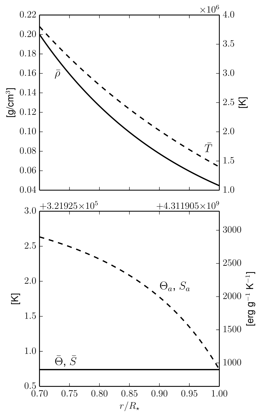
Figure 1: Top panel: Background density $\bar{\rho}$ (left vertical axis) and temperature $\bar{T}$ (right vertical axis) profiles as a function of spherical radius. Bottom panel: Background and ambient potential temperature and entropy profiles. The left vertical axis corresponds to the potential temperature, and the right axis to the entropy.

We consider a fiducial stellar convection zone computed with the EULAG code. The parameters of our fiducial case are indicated in Table 1. We consider a convection zone with a solar-like aspect ratio and which rotates $2.4$ times faster than the Sun, which ensures that the Rossby number $R_{o}=\omega/2\Omega_{0}$ (where $\omega$ is the average vorticity in the middle of the convection zone) remains sufficiently smaller than one, and consequently that the model is strongly influenced by rotation. The background density and temperature profiles are shown in the upper panel of Figure 1. A moderate density contrast (1.5 density scale-heights) is adopted to limit the size of the smallest turbulent scales near the top of the domain. In the lower panel we show the background and ambient potential temperature (and equivalently entropy) profiles. A moderate entropy constrast over the convective shell is chosen to ensure the model is above the critical onset of convection, but remains in an accessible turbulent regime.

The numerical method in EULAG implicitly supplies the dissipation needed to maintain numerical stability, which in turns varies with the grid resolution. We consider two physically identical cases, labelled E1 and E2, in which the grid resolution is respectively $N_{r}\times N_{\theta}\times N_{\varphi}$ = 51 $\times$ 64 $\times$ 128, and 101 $\times$ 128 $\times$ 256, with respective time steps of $900$ and $450$ seconds. By increasing the resolution (in both time and space) by a factor of 2, the implicit dissipation of the numerical scheme of EULAG is expected to be reduced by a factor of 4 (see, e.g., Prusa et al. 2008).

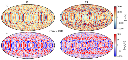
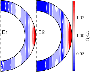
Figure 2: Left panels: Mollweide projections in the middle of the convection zone of the radial velocity (upper panels) and entropy perturbations (lower panels) for cases E1 (left) and E2 (right). The positive $v_{r}$ and $S$ perturbations are denoted in red, and the negative values in blue. Right panels: Differential rotation ($\Omega$) profile (averaged over time and longitude) on the meridional plane for cases E1 (left) and E2 (right). The differential rotation profile is normalized to the stellar rotation rate $\Omega_{\star}$. Rotation faster than $\Omega_{\star}$ is shown in red, slower in blue, and co-rotation appears in white.

We display in Figure 2 the radial velocity and entropy perturbations (left panels) in both cases on a Mollweide projection in the middle of the convection zone. As expected, smaller structures are observed when the resolution is increased. In both cases, the so-called banana cells clearly appear on the equator. Interestingly, the convective luminosity almost does not change between the two cases and peaks at about $0.12\,L_{\odot}$ in the middle of the convection zone. The convective kinetic energy only increases by $10\%$ from E1 to E2, and the temperature perturbations compensate this variation which leads to a very similar convective luminosity. The main difference between the two cases hence lies in the kinetic energy of the differential rotation, which results from the complex interplay of the turbulent scales (through Reynolds stresses) involved in the simulation. The differential rotation (right panels) exhibits a solar-like (fast equator, slow poles) pattern in both cases. Case E2 possesses a significantly stronger pole-equator constrast ($\sim 6\%$) compared to E1 ($\sim 2\%$). The iso-$\Omega$ contours are in both cases mostly parallel to the rotation axis, and an almost co-rotating stripe is observed at mid-to high latitude, indicating that the simulation is indeed in a regime strongly influenced by rotation (low Rossby number).

4 Estimation of the sub-grid scale modelling effects in EULAG

We now quantitatively estimate the effect of the numerical treatment of sub-grid scales in EULAG. We base our analysis on the estimation of energy transfers in the turbulent convection zone simulations. We derive the spectral analysis method in Section  4.1 and detail the results in Section  4.2.

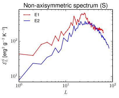
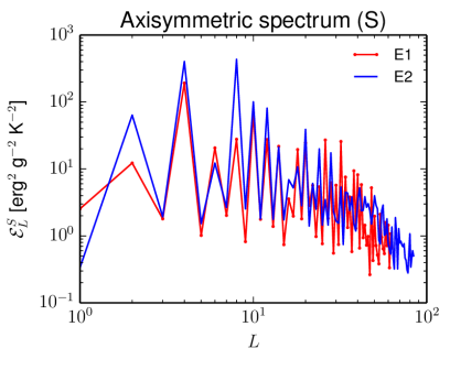
Figure 3: Axisymmetric (left panels) and non-axisymmetric (right panels) kinetic energy (upper panels) and entropy (lower panels) spectra averaged over 40 rotation periods. Case E1 spectra are shown in red and case E2 in blue. The spectra are summed over the spherical harmonics degree $m$ and displayed as a function of $L$ (see text).

4.1 Spectral Analysis: Method

We analyze the results from the EULAG code with the help of a spectral analysis of energy transfers between scales in the spherical harmonics space. This method was originally developed in Strugarek et al. (2013) in the context of characterizing the transfer of magnetic energy between scales in dynamo simulations. It was more recently adapted to the EULAG code to study the self-consistent development of MHD instabilities in the solar tachocline (Lawson et al. 2015). We extend it here to study kinetic energy and entropy spectral transfers (we refer the reader to Strugarek et al. 2013, and to A for more details about this spectral analysis method). The scalar and vectorial quantities are respectively projected on the standard and vectorial spherical harmonics bases (Rieutord 1987)

$$Y_{l}^{m}=\sqrt{\frac{(2l+1)}{4\pi}\frac{(l-|m|)!}{(l+|m|)!}}P^{|m|}_{l}(\cos\theta)e^{im\varphi}$$ (17)

and

$$\left\{\begin{array}[]{lcl}\mathbf{R}_{l}^{m}&=&Y_{l}^{m}{\bf e}_{r}\\ \mathbf{S}_{l}^{m}&=&\partial_{\theta}Y_{l}^{m}{\bf e}_{\theta}+\frac{1}{\sin{\theta}}\partial_{\varphi}Y_{l}^{m}{\bf e}_{\varphi}\\ \mathbf{T}_{l}^{m}&=&\frac{1}{\sin{\theta}}\partial_{\varphi}Y_{l}^{m}{\bf e}_{\theta}-\partial_{\theta}Y_{l}^{m}{\bf e}_{\varphi}\end{array}\right.\,,$$ (21)

where $P^{m}_{l}$ are the Legendre polynomials.

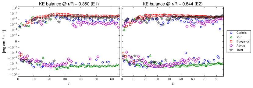
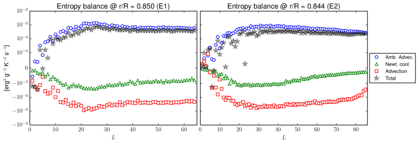
Figure 4: Kinetic energy (upper panels) and entropy (lower panels) balance Equations (24)-(25) for cases E1 (left panels) and E2 (right panels), in the middle of the convection zone. For each equation the various terms are labeled with a coloured symbol, and the total of all the contributions is shown by the gray transparent stars.

We define the kinetic energy and entropy spectra by

$$\mathcal{E}^{K}_{L}(r)= \frac{1}{2}\bar{\rho}\iint{\bf u}_{L}\cdot{\bf u}_{L}^{cc}{\rm d}\Omega\,,$$ (22)

$$\mathcal{E}^{S}_{L}(r)= \frac{1}{2}\iint S_{L}\cdot S_{L}^{cc}{\rm d}\Omega\,,$$ (23)

where ${\rm d}\Omega=\sin\theta{\rm d}\theta{\rm d}\varphi$ and the exponent ^cc denotes the complex conjugate. The subscript $L$ corresponds to the sum over the subset of spherical harmonics coefficients $(l,m)$ with fixed $l$ and $m$ restricted to a chosen ensemble $\mathcal{M}$. In this work we will consider the two ensembles $\mathcal{M}_{0}=\{m=0\}$ and $\mathcal{M}_{\star}=\{m\in[-l,l],\,m\neq 0\}$. We display those axisymmetric and non-axisymmetric spectra at mid-depth for cases E1 and E2 in Figure 3. The axisymmetric kinetic energy spectrum (upper left panel) is dominated by the differential rotation that populates the odd $L$ components of the spectrum. The entropy axisymmetric spectrum (lower left panel) is conversely dominated by even $L$ components, which correspond to the mean pole-equator temperature contrast that establishes itself in the simulations. The non-axisymmetric kinetic energy spectrum (upper right panel) exhibits a peak around $L\sim 25$ in case E1 ($L\sim 35$ in case E2) which corresponds to the dominant convective structure that can be observed in the Mollweide projection in Figure 2. As expected, the non-axisymmetric kinetic energy spectrum at scales $L>20$ is shifted to smaller scales (higher $L$’s) when the resolution is increased, but the overall shape of the non-axisymmetric kinetic energy spectrum remains the same. The non-axisymmetric entropy spectrum peaks at $L\sim 25$ in case E1 and $L\sim 30$ in case E2. When the resolution is doubled, the entropy spectrum is not shifted to smaller scales but the negative slope extends down to the smallest scales resolved in the domain.

Using the anelastic Equations (2) and (3) with no explicit dissipation, we obtain the following evolution equations

$$\dot{\mathcal{E}}^{K}_{L}(r)= \mathcal{P}_{L}+\mathcal{G}_{L}+\mathcal{C}_{L}+\sum_{L_{1},L_{2}}\mathcal{R}_{L}\left(L_{1},L_{2}\right)\,,$$ (24)

$$\dot{\mathcal{E}}^{S}_{L}(r)= \mathcal{S}^{a}_{L}+\mathcal{N}_{L}+\sum_{L_{1},L_{2}}\mathcal{A}_{L}\left(L_{1},L_{2}\right)\,.$$ (25)

In the kinetic energy Equation (24), the various terms in the right hand side correspond to contributions from the pressure gradient, buoyancy, Coriolis force and non-linear advection of momentum. Note that the Coriolis contribution $\mathcal{C}_{L}$ vanishes when summed over all scales $L$ as it should, but is able to spectrally redistribute energy among neighbour shells (see also Augier and Lindborg 2013 and A.2.2). In the entropy Equation (25), they correspond to the ambient state advection, Newtonian cooling, and non-linear advection of the entropy perturbations. The detailed expressions of the different terms can be found in A.2 and A.3. We show in Figure 4 the various terms of Equations (24) and (25) for cases E1 and E2 at mid-depth (we focus here solely on the non-axisymmetric spectra). The different contributions are averaged over more than 40 stellar rotations after the simulations have reached a steady-state (i.e. after the total kinetic energy is stabilized). In the kinetic energy balance (upper panels), buoyancy (red squares) is clearly the source of energy for almost all turbulent scales and is generally opposed by the pressure gradient (green triangles). The non-linear advection contribution (magenta diamonds) changes sign at the peak of the spectrum because of a direct energy cascade: scales larger than the maximum energy scale lose energy to the smaller scales. The Coriolis force (blue circles) efficiently acts on the largest scales due to the small latitudinal extent of the higher $L$ modes, as expected.

The entropy balance is shown in the lower panels. The entropy perturbations draw energy from the ambient entropy profile at all scales (blue circles) and are stabilized by the non-linear advection (red squares). The Newtonian cooling term (green triangles) contributes very marginally to the entropy balance since we chose a long cooling timescale $\tau$ (see Table 1). We finally note that no cascading process is observed in the entropy transfers in these numerical experiments: the non-linear advection is negative for all the resolved scales.

The total right hand side of the kinetic energy and entropy evolution equations —shown as gray stars in Figure 4— should cancel out in steady-state. In Figure 4, we recall that the various contributions were averaged over a time period of 40 stellar rotations during which the total energy in the system has stabilized. Hence, the system is in steady-state and the imbalance (gray stars) can only be attributed to the effect of the numerical scheme that we do not represent in these plots and that tends to dissipate energy in EULAG. We now propose a possible interpretation of this imbalance to obtain quantitative estimates of the effect of the sub-grid scales modelling in EULAG.

4.2 Effective dissipation coefficients

In EULAG, the implicit treatment of sub-grid scales results in an additional contribution to the kinetic energy and entropy evolution equations that is a priori unknown. In the context of 3D homogeneous turbulence in a cartesian box, Domaradzki et al. (2003) showed that the implicit sub-grid scales treatment of MPDATA (the numerical algorithm behind EULAG) mimics qualitatively an eddy viscosity. We build here on this idea and attempt to match the unknown additional terms of Equations (24) and (25) to an eddy viscosity and an eddy thermal dissipation. Such dissipation terms can be written as

$$\mathcal{V}_{L}= \iint\left(-\boldsymbol{\nabla}\cdot\boldsymbol{\mathcal{D}}\right)_{L}\cdot\mathbf{u}_{L}\,{\rm d}\Omega\,,$$ (26)

$$\mathcal{K}_{L}= \iint\left(Q_{\kappa}\right)_{L}\cdot S_{L}\,{\rm d}\Omega\,,$$ (27)

where $\boldsymbol{\mathcal{D}}$ and $Q_{\kappa}$ respectively depend on an eddy viscosity $\nu$ and an eddy thermal dissipation coefficient $\kappa$ (Equations 4 and 5). Using the results from EULAG simulation, we calculate Equations (26) and (27) neglecting at this point the dependency upon radius and scale $L$ of the unknown dissipation coefficients $\nu$ and $\kappa$ (set to arbitrary values $\nu_{a}=1$, $\kappa_{a}=1$). Our procedure to obtain effective dissipation coefficient is as follows. We average in time the right hand side of Equation (24) (the left hand side is vanishingly small because the system has reached a statistical steady-state), and divide it with the analogously averaged Equation (26). The resulting ratio gives us naturally $\nu_{\rm eff}$. The exact same procedure is applied to Equations (25) and (27) to obtain $\kappa_{\rm eff}$. We display the resulting eddy-diffusion coefficients $\nu_{\rm eff}(r,L)$ and $\kappa_{\rm eff}(r,L)$ in the left panels of Figure 5 for case E1.

Our numerical procedure embeds numerous numerical approximations that need to be acknowledged. First, we have no formal proof that the numerical sub-grid scales effects can be matched to an eddy-type dissipation in the case of turbulent convection simulations with EULAG. Second, EULAG is formulated on a regular cartesian grid which is mapped to the spherical geometry. Here, we carry our analysis on a spherical harmonics decomposition that is obtained through an interpolation of EULAG’s results on Gauss-Legendre collocation points in latitude. Hence, some numerical errors can appear in our analysis since this does not reflect directly how Equations (1)-(3) are solved in EULAG. Third, the spherical harmonics decomposition is cut at the maximum accessible spherical harmonics degree $L_{\rm max}$, corresponding to the smallest grid size in latitude in EULAG. We repeated our analysis by de-aliasing the spherical harmonics decomposition up to $2L_{\rm max}/3$, which did not significantly change our results, giving us confidence that the second and third error sources are not significantly affecting our study. Finally, because we cannot expect the sub-grid scale model to behave entirely as an eddy-type dissipation operator, we consider a criterion to assess the robustness of the effective eddy-dissipation coefficients we obtained. For each value of $\nu_{\rm eff}(r,L)$ (and $\kappa_{\rm eff}(r,L)$), we calculate the standard deviation along the time window over which we averaged the various contributions shown in Figure 4. If the standard deviation is of the order of the deduced eddy-dissipation coefficient, we do not confidently rely on its value. In the left panels of Figure 5 we darken the pixels of the $(r,L)$ colormaps accordingly, and only consider the bright pixels in the following analysis.

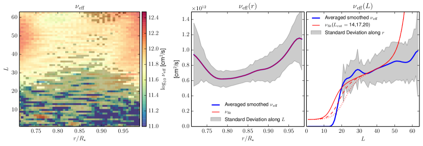
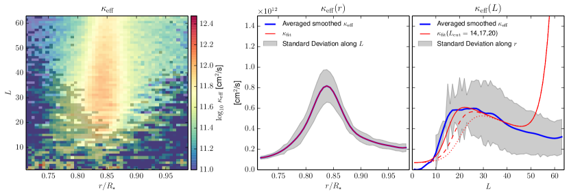
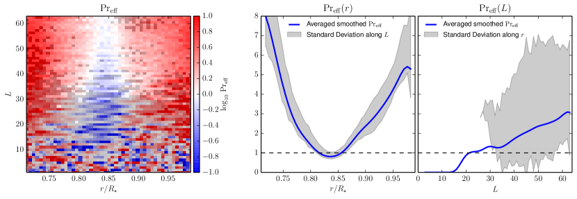
Figure 5: Left panels: Effective visocity $\nu_{\rm eff}$ (upper panel), heat dissipation coefficient $\kappa_{\rm eff}$ (middle panel) and Prandtl number $Pr$ (lower panel), as a function of spherical radius and spherical harmonics degree $L$. The colormap in each panel is displayed on a logarithmic scale. In each panel, gray pixels label non-robust effective dissipation coefficients (see text). Note that in the lower panel, white areas correspond to an effective Prandtl number of unity. Right panels: Averaged, smoothed profiles (blue lines) as a function of spherical radius (left) and spherical harmonics degree $L$ (right). The gray area corresponds to the standard deviation of the effective dissipation coefficients around the average value. The red lines denote the fitted dissipation coefficients that are used in ASH simulations in Section  4.3. In the lower panel, the Prandtl number of unity is labeled by the horizontal dashed black line.

The robust eddy-diffusion coefficients show characteristic patterns in $r$ and $L$, which are shown in the right panels of Figure 5. The eddy viscosity is maximized near the radial boundaries (which are impenetrable), and increases with $L$. Its average value lies between $5\times 10^{11}$ cm²/s and $1.5\times 10^{12}$ cm²/s which agrees with empirically deduced implicit eddy-diffusion coefficients obtained with mean-field models representing EULAG simulations (see, e.g., Simard et al. 2016). The average profile in $r$ and $L$ are shown in blue, and the standard deviation along $L$ and $r$ is denoted by the gray areas.

The eddy heat dissipation coefficient shows a reversed profile. It is maximized at the center of the convection zone and decreases strongly (by almost a factor of 8) close to the radial boundaries. In the robust part of the $L$ profile ($L\geq 20$) it decreases with $L$.

The lower panels show the effective Prandtl number ${\rm Pr}_{\rm eff}=\nu_{\rm eff}/\kappa_{\rm eff}$. It is generally assumed in ILES that the Prandtl number is close to $1$. Here we find that it is indeed very close to unity in the middle of the convection zone (${\rm Pr}_{\rm eff}=1$ corresponds to white in the colormap), but rapidly increases by almost an order of magnitude near the radial boundaries. The Prandtl number also slightly increases with $L$, due to the simultaneous increase of $\nu_{\rm eff}$ and decrease of $\kappa_{\rm eff}$.

We performed the same analysis for case E2, which is not shown here. The radial profile of the dissipation coefficients is very similar to the one shown in Figure 5, and the $L$ profile is simply shifted to higher $L$’s thanks to the finer resolution. The average value of $\nu_{\rm eff}$ and $\kappa_{\rm eff}$ is decreased by factor between $3$ and $5$, which is compatible with the naive expectation of doubling the overall resolution (in both time and space) of the simulation, leading to an implicit dissipation reduced by a factor of 4.

4.3 Comparison with the ASH code

In order to further validate the deduced dissipation coefficients, we now use them in LES done with the ASH code. The ASH code allows to specify dissipation coefficient depending on both $r$ and $L$, which enables to fully take into account the dissipation coefficients inverted in Section  4.2.

We fit the dissipation coefficients with the following formulation

$$\nu_{\rm fit}(r,L)= \nu_{m}\left(b_{\nu}L+c_{\nu}\right)\sum_{k=0}^{N}a^{\nu}_{k}\left(\frac{r}{R_{\star}}\right)^{k}$$ (28)

$$\kappa_{\rm fit}(r,L)= \kappa_{m}\left(b_{\kappa}L+c_{\kappa}\right)\sum_{k=0}^{N}a^{\kappa}_{k}\left(\frac{r}{R_{\star}}\right)^{k}\,.$$ (29)

The radial shape of the effective dissipation coefficients is fitted with a standard polynomial. The dependency against $L$ is fitted only in the $L\in[20,L_{\rm max}]$ range because the matched $\nu_{\rm eff}$ and $\kappa_{\rm eff}$ are not statistically significant at low $L$ (see the discussion in previous section). We linearly fit both of them for the sake of simplicity.

At large scales, dissipation is small in EULAG and our method is not able to match EULAG’s dissipation to standard enhanced dissipation coefficients. In ASH, we hence arbitrarily set them to the small values $\nu_{l}=2\times 10^{11}$ cm²/s and $\kappa_{l}=5\times 10^{10}$ cm²/s using a smooth hyperbolic tangent (red curves in Figure 5). Furthermore, an ASH simulation using these fitted coefficients is not stable when using the same grid resolution as in EULAG. Hence, we double the resolution of case E1 in ASH and arbitrarily increase the value of the fitted coefficients to $\nu_{s}=10^{13}$ cm²/s and $\kappa_{s}=2\times 10^{13}$ cm²/s at small scales (large $L$), using again a smooth hyperbolic tangent. The fitted profiles used in ASH are shown in red in the middle and right panels of Figure 5, and can be written as (here, for the viscosity)

$$\nu(r,L)=\left[\nu_{\rm fit}+(1-s_{l})\nu_{l}\right]\left(1-s_{s}\right)+s_{s}\nu_{s}\,,$$ (30)

where the subscripts $s$ and $l$ respectively refer to the small and large scale branches of the profile, and the generic step function $s(L,L_{i})$ is defined by

$$s(L,L_{i})=\frac{1}{2}\left[1+\tanh\left(\frac{L-L_{i}}{0.1\,L_{i}}\right)\right]\,,$$ (31)

where $L_{i}$ is centering parameter of the hyperbolic tangent.

The ASH results are sensitive to the arbitrary choices of effective dissipation coefficients at large and small scales. In order to illustrate their sensitivity, we show three different cases obtained with ASH when the transition at large scales is slightly shifted (see the solid, dashed and dotted red lines in Figure 5). We label the cases ’A$L_{l}$’ where $L_{l}$ is the centering scale of the hyperbolic tangent at large scales. At small scales, the centering scale is set to $L_{s}=64$ for all cases. Figure 6 shows the resulting differential rotation, its radial profiles at various latitudes, and the radial velocity at mid depth, correspondingly for the three cases together with the case E1.

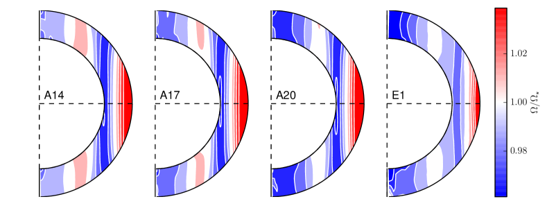
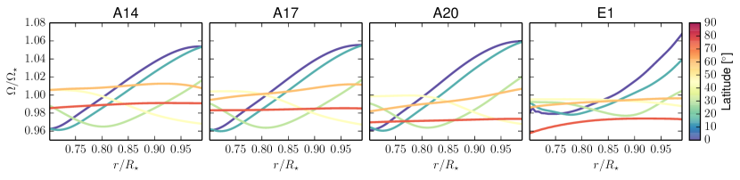
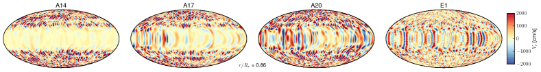
Figure 6: Upper panels Differential rotation for the three ASH cases (see red curves in Figure 5) and case E1. As in Figure 2, blue and red respectively denote slower and faster rotation than the stellar rotation rate shown in white. Middle panels Radial profile of the differential rotation at five different latitudes in the northern hemisphere. The profile at the equator is in blue, and at $75^{\circ}$ latitude in red (see color bar). Lower panels Radial velocity colormap at the middle of the convection zone for the ASH cases and case E1. Again, red denotes outward motions and blue downward motions.

The three cases exhibit a differential rotation pattern which qualitatively agrees with case E1. Overall, case A20 matches E1 best, albeit its differential rotation is stronger, and steeper at the equator (blue line). However, A20 better matches E1 at mid latitudes (yellow to red lines) where A14 and A17 evince too strong differential rotation.

The convective patterns (lower panels) change significantly between the three cases. In case A14, convection is very weak on an equatorial band and is concentrated at higher latitudes. In case A17 only an “active nest of convection” (see Brown et al. 2008) is observed on the equator, and in case A20 the convective patterns qualitatively match E1 with slightly stronger convective amplitudes. We recall that the only difference between cases A14 and A20 is the location of the transition to low dissipation coefficients at large scales, i.e. in case A20 a larger range of large scales is evolved with low dissipation coefficients. We recall that the kinetic energy spectrum peaks in between $L=20$ and $L=30$ in the ASH cases. The non-linear balance saturating the peak of the turbulent convective spectrum is thus altered from left to right in Figure 6, with higher viscous and heat dissipation in case A14 than in case A20 at the peak of the turbulent spectrum. In case A14, the radial shear of the differential rotation near the equatorial plane is strong enough to weaken significantly convection, whereas in case A20 the banana cells still live on.

In spite of these differences, the three ASH cases exhibit a similar convective heat transport (not shown) peaked at the center of the convection zone with an equivalent convective luminosity $L_{\rm cz}\sim 0.14\,L_{\odot}$ in cases A17 and A20, and $L_{\rm cz}\sim 0.13\,L_{\odot}$ in case A14. All three are close to the E1 case, for which the convective transport reaches $0.12L_{\odot}$ (see Section 3).

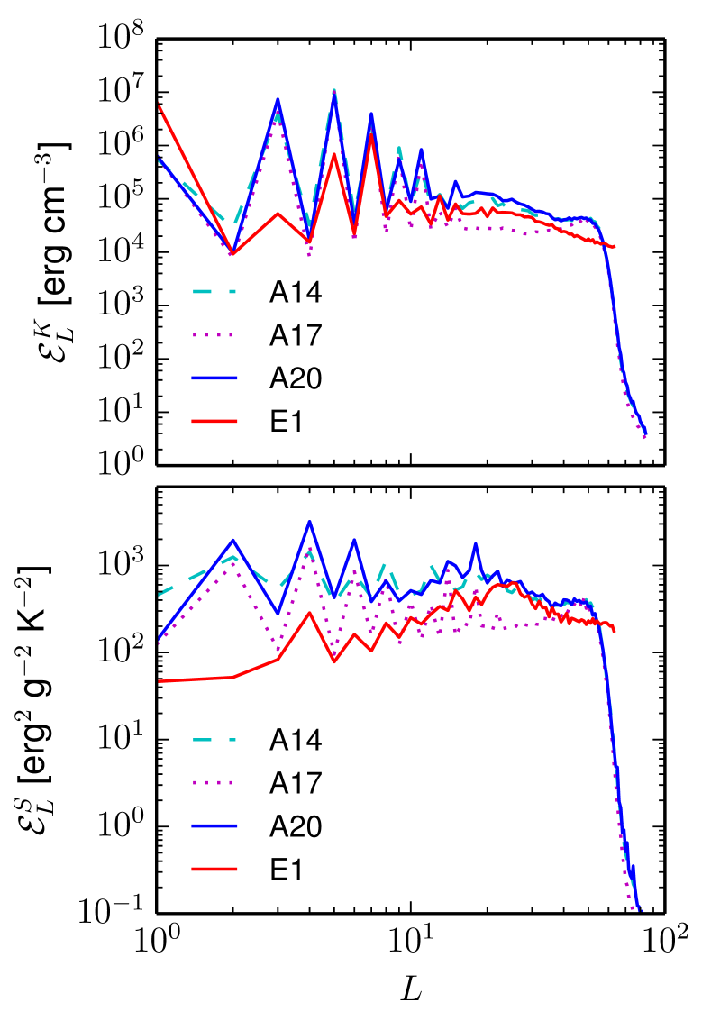
Figure 7: Total kinetic energy (top panel) and entropy (bottom panel) spectra for cases A14 (dashed cyan), A17 (dotted magenta), A20 (plain blue) and E1 (plain red).

Interestingly, the large-scale non-axisymmetric entropy spectrum (Figure 7) is significantly larger in ASH cases compared to EULAG, while the kinetic energy spectrum at those scales remain the same. The slope of the kinetic energy spectrum at mid-scale in EULAG is well recovered by case A20, with a departure near the transition to high dissipation around $L=64$. The change in the spectra from case A14 to case A20 denotes a non-trivial influence of scale-dependent dissipation coefficients on the correlations between the large-scale heat and momentum fluctuation. This may have important theoretical implications for the amplitude of the large-scale convective fluctuations in the Sun (Hanasoge et al. 2012; Greer et al. 2015; Lord et al. 2014), and will be studied in near future.

Finally, we recall that the viscous heating has been omitted in the governing equations, as in ILES it is generally not accounted for by numerics supplying small-scale diffusion, and hence should not be formally introduced in this ILES-LES comparison. Nevertheless, omitting the viscous heating could formally lead to net energy loss in simulations, we hence intend to explore this effect in a subsequent study.

Numerous numerical approximations have been made in (i) projecting the results from EULAG in spectral space, (ii) matching the imbalance in Equations (24) and (25) to standard laplacian dissipation terms, and (iii) using the matched dissipations coefficients in a LES with the ASH code, introducing arbitrary dissipation coefficients at very large and very small scales. In spite of these approximations, we managed to simulate with ASH (case A20), using fitted explicit dissipation coefficients, a convective state producing a large scale differential rotation that compares adequately with the results obtained with EULAG. This comparison gives us confidence in the methodology we developed to estimate the dissipation properties of ILES with EULAG, and a posteriori suggests that, at least in the bulk part of the turbulent spectrum, EULAG’s implicit dissipation could be interpreted in terms of standard explicit dissipation.

5 Conclusions

In this work we have studied the dissipation properties of implicit large-eddy simulations of an idealized turbulent stellar convection zone under the influence of rotation with the EULAG code. By considering twin simulations where the grid resolution was doubled, we showed that the kinetic energy spectrum of turbulent convection peaks at smaller scales in the most refined model, as expected. The latter model develops a stronger differential rotation, which results from the complex interplay between the turbulent scales, which are themselves affected by the implicit dissipation of EULAG.

In order to characterize this implicit dissipation, we developed a spectral method to a posteriori quantify the effect of the sub-grid scale modelling of EULAG. By evaluating balance equations for kinetic energy and entropy when the system has reached a steady-state, we were able to isolate the implicit dissipation contribution. The sub-grid scale modelling was shown to match quantitatively well a standard laplacian-like operator from medium to small scales. At large scales, the implicit dissipation introduced by EULAG is very weak and could not be matched to such classical formulation.

For a grid resolution comparable to previously published results with EULAG in the context of solar dynamo (Ghizaru et al. 2010; Racine et al. 2011; Beaudoin et al. 2013; Passos and Charbonneau 2014; Lawson et al. 2015), we find the effective viscosity and thermal diffusivities are of the order of $10^{12}$ cm²/s. However, we recall that the effective dissipation does not match to an equivalent enhanced dissipation coefficient for the large scales feature such as differential rotation, for which we showed the effective dissipation to be a least an order of magnitude lower.

In order to further test our estimates of the dissipation coefficients, we used them in a series of LES with the ASH code. Note however that we were compelled to select arbitrary dissipation coefficients at very small scales (below the EULAG grid scale) and very large scales (where the implicit dissipation in EULAG is small and does not match a standard laplacian operator). We showed that our arbitrary choice of dissipation coefficients at large scale could significantly affect the large-scale flows in ASH. However, by choosing adequately these dissipation coefficients, we were able to reproduce the large scale differential rotation of EULAG simulation. Our results thus indicate that results from ILES and LES could be reconciled.

The spectral analysis developed in this paper is generic and can be easily extended to the MHD regime (Strugarek et al. 2013). A natural extension of this work is to perform such joint simulations of cyclic dynamos, in order to isolate to what extent the particular treatment of sub-grid scales chosen in EULAG simulations impacts the existence and characteristics of such solutions, as well as their dependency to rotation. We intend to explore this aspect in a future publication.

References

Appendix A Spectral transfers equations

A.1 Vectorial spherical harmonics basis

A.1.1 The standard vectorial basis

We define from Rieutord (1987); Mathis and Zahn (2005):

$$\left\{\begin{array}[]{lcl}\mathbf{R}^{m}_{l}&=&Y_{l}^{m}\mathbf{e}_{r}\\ \mathbf{S}^{m}_{l}&=&\partial_{\theta}Y_{l}^{m}\mathbf{e}_{\theta}+\frac{1}{\sin{\theta}}\partial_{\varphi}Y_{l}^{m}\mathbf{e}_{\varphi}\\ \mathbf{T}^{m}_{l}&=&\frac{1}{\sin{\theta}}\partial_{\varphi}Y_{l}^{m}\mathbf{e}_{\theta}-\partial_{\theta}Y_{l}^{m}\mathbf{e}_{\varphi}\end{array}\right.,$$ (35)

where $(\mathbf{e}_{r},\mathbf{e}_{\theta},\mathbf{e}_{\varphi})$ defines the spherical basis and $Y^{m}_{l}$ are the spherical harmonics defined by

$$Y_{l}^{m}=\sqrt{\frac{(2l+1)}{4\pi}\frac{(l-|m|)!}{(l+|m|)!}}P^{|m|}_{l}(\cos\theta)e^{im\varphi}\,$$ (36)

where $P^{m}_{l}$ are the associated Legendre polynomials. The basis (35) have the following properties :

$$\iint\mathbf{R}^{m_{1}}_{l_{1}}\cdot\left(\mathbf{R}^{m_{2}}_{l_{2}}\right)^{cc}{\rm d}{\Omega}{}= \delta_{l_{1},l_{2}}\delta_{m_{1},m_{2}},$$ (37)

$$\iint\mathbf{S}^{m_{1}}_{l_{1}}\cdot\left(\mathbf{S}^{m_{2}}_{l_{2}}\right)^{cc}{\rm d}{\Omega}{}= \iint\mathbf{T}^{m_{1}}_{l_{1}}\cdot\left(\mathbf{T}^{m_{2}}_{l_{2}}\right)^{cc}{\rm d}{\Omega}{}$$

$$= l_{1}(l_{1}+1)\delta_{l_{1},l_{2}}\delta_{m_{1},m_{2}},$$ (38)

where ${\rm d}{\Omega}{}=\sin\theta\mbox{d}\theta\mbox{d}\varphi$ the solid angle, $cc$ means complex conjugate and $\delta$ is the Kronecker symbol. We also have:

$$(\mathbf{S}^{m}_{l})^{cc}=(-1)^{m}\mathbf{S}^{-m}_{l}\,,$$ (39)

and all the other scalar cross products are $0$.

A.1.2 Scalar fields identities

Defining $\psi=\sum_{l,m}\left\{\psi_{m}^{l}(r)Y_{l}^{m}\right\}$, we get:

$$\nabla\psi= \sum_{l,m}\left\{\partial_{r}\psi_{m}^{l}\mathbf{R}^{m}_{l}+\frac{\psi_{m}^{l}}{r}\mathbf{S}^{m}_{l}\right\},$$ (40)

$$\nabla\cdot\nabla\psi= \sum_{l,m}\Delta_{l}\psi_{m}^{l}Y_{l}^{m}$$ (41)

where $\Delta_{l}=\partial^{2}_{rr}+\frac{2}{r}\partial_{r}-\frac{l(l+1)}{r^{2}}$.

A.1.3 Vectorial fields identities

For a vector

$$\mathbf{X}=\sum_{l,m}\left\{\mathcal{A}^{l}_{m}\mathbf{R}^{m}_{l}+\mathcal{B}^{l}_{m}\mathbf{S}^{m}_{l}+\mathcal{C}^{l}_{m}\mathbf{T}^{m}_{l}\right\}\,,$$

we obtain:

$$\nabla\cdot\mathbf{X}= \sum_{l,m}\left[\frac{1}{r^{2}}\partial_{r}(r^{2}\mathcal{A}^{l}_{m})-l(l+1)\frac{\mathcal{B}^{l}_{m}}{r}\right]Y_{l}^{m}\,,$$ (42)

$$\nabla\times\mathbf{X}= \sum_{l,m}\left[l(l+1)\frac{\mathcal{C}^{l}_{m}}{r}\right]\mathbf{R}^{m}_{l}$$

$$+\left[\frac{1}{r}\partial_{r}(r\,\mathcal{C}^{l}_{m})\right]\mathbf{S}^{m}_{l}$$

$$+\left[\frac{\mathcal{A}^{l}_{m}}{r}-\frac{1}{r}\partial_{r}(r\,\mathcal{B}^{l}_{m})\right]\mathbf{T}^{m}_{l}\,,$$ (43)

$$\nabla^{2}\mathbf{X}= +\left[\Delta_{l}\mathcal{A}^{l}_{m}-\frac{2}{r^{2}}(\mathcal{A}^{l}_{m}-l(l+1)\mathcal{B}^{l}_{m})\right]\mathbf{R}^{m}_{l}$$

$$+\sum_{l,m}\left[\Delta_{l}\mathcal{B}^{l}_{m}+2\frac{\mathcal{A}^{l}_{m}}{r^{2}}\right]\mathbf{S}^{m}_{l}$$

$$+\left[\Delta_{l}\,\mathcal{C}^{l}_{m}\right]\mathbf{T}^{m}_{l}\,.$$ (44)

A.1.4 An alternative vectorial basis

The vectorial spherical harmonics basis defined in appendix A.1 is very efficient to calculate scalar products or linear differential operator on vectors. Nevertheless, it is quite hard to use it to express vectorial products. Instead we define the following basis (e.g., see Varshalovich et al. 1988):

$$\mathbf{Y}_{l,l+\nu}^{\hskip 2.84544ptm}=\sum_{\mu=-1}^{1}(-1)^{l-m}c_{l,m,\nu,\mu}Y_{l+\nu}^{m-\mu}\mathbf{e}_{\mu}\,,$$ (45)

where

$$c_{l,m,\nu,\mu}=\sqrt{2l+1}\left(\begin{array}[]{ccc}l&l+\nu&1\\ m&\mu-m&-\mu\end{array}\right)\,,$$ (48)

$(\dots)$ is the $3$-j Wigner coefficient linked to Clebsch-Gordan coefficients, and the vectors $\mathbf{e}_{\mu}$ are

$$\left\{\begin{array}[]{lcl}\mathbf{e}_{-1}&=&\frac{1}{\sqrt{2}}\left(\mathbf{e}_{x}-i\mathbf{e}_{y}\right)\\ \mathbf{e}_{0}&=&\mathbf{e}_{z}\\ \mathbf{e}_{1}&=&-\frac{1}{\sqrt{2}}\left(\mathbf{e}_{x}+i\mathbf{e}_{y}\right)\end{array}\right.,$$ (52)

where $(\mathbf{e}_{x},\mathbf{e}_{y},\mathbf{e}_{z})$ defines the cartesian basis. Note that the equivalent of the conjugation rule (39) is then

$$\left(\mathbf{Y}^{m}_{l,l+\nu}\right)^{cc}=\left(-1\right)^{m+\delta_{0\nu}}\mathbf{Y}^{-m}_{l,l+\nu}\,.$$ (53)

A.1.5 Vectorial product

As previously, we decompose a vector $\mathbf{X}$ on this basis:

$$\mathbf{X}=\sum_{l=0}^{\infty}\sum_{m=-l}^{l}\sum_{\nu=-1}^{1}X_{l,l+\nu}^{\hskip 2.84544ptm}\mathbf{Y}_{l,l+\nu}^{\hskip 2.84544ptm}.$$

Evaluating the vectorial product of two vectors $\mathbf{X}_{0}=\mathbf{X}_{1}\times\mathbf{X}_{2}$, one gets:

$$X_{0;l_{0},l_{0}+\nu_{0}}^{\hskip 2.84544ptm_{0}}= \sum_{\begin{subarray}{c}l_{1},l_{2}=0\\ l_{0}\geq|l_{1}-l_{2}|\\ l_{0}\leq l_{1}+l_{2}\end{subarray}}^{\infty}\sum_{\begin{subarray}{c}m_{1}=-l_{1}\\ m_{2}=-l_{2}\\ m_{1}+m_{2}=m_{0}\end{subarray}}^{l_{1},l_{2}}\sum_{\nu_{1},\nu_{2}}$$

$$X_{1;l_{1},l_{1}+\nu_{1}}^{\hskip 2.84544ptm_{1}}X_{2;l_{2},l_{2}+\nu_{2}}^{\hskip 2.84544ptm_{2}}\mathcal{J}^{l_{0},m_{0},\nu_{0}}_{l_{1},m_{1},\nu_{1},l_{0},m_{0},\nu_{0}},$$ (54)

where

$$\mathcal{J}^{l,m_{1}+m_{2},\nu}_{l_{1},m_{1},\nu_{1},l_{2},m_{2},\nu_{2}}=i(-1)^{\nu_{1}-\nu_{2}+(m_{1}+m_{2})}\sqrt{\frac{3}{2\pi}}$$

$$\sqrt{(2l_{1}+1)(2l_{1}+2\nu_{1}+1)(2l_{2}+1)(2l_{2}+2\nu_{2}+1)}$$

$$\sqrt{(2l+1)(2l+2\nu+1)}\left\{\begin{array}[]{ccc}l_{1}&l_{2}&l\\ l_{1}+\nu_{1}&l_{2}+\nu_{2}&l+\nu\\ 1&1&1\end{array}\right\}$$ (58)

$$\left(\begin{array}[]{ccc}l_{1}&l_{2}&l\\ m_{1}&m_{2}&-(m_{1}+m_{2})\end{array}\right)$$ (61)

$$\left(\begin{array}[]{ccc}l_{1}+\nu_{1}&l_{2}+\nu_{2}&l+\nu\\ 0&0&0\end{array}\right),$$ (64)

with $\{\cdots\}$ being the $9$-j Wigner coefficient.

A.1.6 Scalar product

We decompose a vector $\mathbf{X}$ on this basis in the following way:

$$\mathbf{X}=\sum_{l=0}^{\infty}\sum_{m=-l}^{l}\sum_{\nu=-1}^{1}X_{l,l+\nu}^{\hskip 2.84544ptm}(r)\mathbf{Y}_{l,l+\nu}^{\hskip 2.84544ptm}.$$

Evaluating the scalar product of two vectors $\mathcal{M}=\mathbf{X}_{1}\cdot\mathbf{X}_{2}$, one gets:

$$\mathcal{M}^{l}_{m}=\sum_{\begin{subarray}{c}l_{1},m_{1},\nu_{1}\\ l_{2},m_{2},\nu_{2}\\ m_{1}+m_{2}=m\end{subarray}}X_{1;l_{1},l_{1}+\nu_{1}}^{\hskip 2.84544ptm_{1}}X_{2;l_{2},l_{2}+\nu_{2}}^{\hskip 2.84544ptm_{2}}\mathcal{H}^{l,m_{1}+m_{2}}_{l_{1},m_{1},\nu_{1},l_{2},m_{2},\nu_{2}}$$ (65)

where the sum symbol is the same as in Equation (54) and

$$\mathcal{H}^{l,m_{1}+m_{2}}_{l_{1},m_{1},\nu_{1},l_{2},m_{2},\nu_{2}}=(-1)^{l_{1}-(l_{2}+\nu_{2})+l+m}\sqrt{\frac{1}{4\pi}}$$

$$\sqrt{(2l_{1}+1)(2l_{1}+2\nu_{1}+1)}$$

$$\sqrt{(2l_{2}+1)(2l_{2}+2\nu_{2}+1)(2l+1)}$$

$$\left\{\begin{array}[]{ccc}l_{1}+\nu_{1}&l_{2}+\nu_{2}&l\\ l_{2}&l_{1}&1\end{array}\right\}$$ (68)

$$\left(\begin{array}[]{ccc}l_{1}&l_{2}&l\\ m_{1}&m_{2}&-(m_{1}+m_{2})\end{array}\right)$$ (71)

$$\left(\begin{array}[]{ccc}l_{1}+\nu_{1}&l_{2}+\nu_{2}&l\\ 0&0&0\end{array}\right)$$ (74)

with $\{\cdots\}$ being here the $6$-j Wigner coefficient.

A.1.7 Basis change relations

For a vector $\mathbf{X}$ decomposed in the following manner:

$$\mathbf{X}= \sum_{l,m}\left\{\mathcal{A}^{l}_{m}\mathbf{R}^{m}_{l}+\mathcal{B}^{l}_{m}\mathbf{S}^{m}_{l}+\mathcal{C}^{l}_{m}\mathbf{T}^{m}_{l}\right\}$$

$$= \sum_{l=0}^{\infty}\sum_{m=-l}^{l}\sum_{\nu=-1}^{1}\left\{X_{l,l+\nu}^{\hskip 2.84544ptm}\mathbf{Y}_{l,l+\nu}^{\hskip 2.84544ptm}\right\},$$

we have the two following relations to change from one basis to the other:

$$\left\{\begin{array}[]{lcl}\mathcal{A}^{l}_{m}&=&\frac{1}{\sqrt{2l+1}}\left[\sqrt{l}X_{l,l-1}^{\hskip 2.84544ptm}-\sqrt{l+1}X_{l,l+1}^{\hskip 2.84544ptm}\right]\\ \mathcal{B}^{l}_{m}&=&\frac{1}{\sqrt{2l+1}}\left[\frac{1}{\sqrt{l}}X_{l,l-1}^{\hskip 2.84544ptm}+\frac{1}{\sqrt{l+1}}X_{l,l+1}^{\hskip 2.84544ptm}\right]\\ \mathcal{C}^{l}_{m}&=&\frac{i}{\sqrt{l(l+1)}}X_{l,l}^{\hskip 2.84544ptm}\end{array}\right.\,,$$ (78)

$$\left\{\begin{array}[]{lcl}X_{l,l-1}^{\hskip 2.84544ptm}&=&\sqrt{\frac{l}{2l+1}}\left(\mathcal{A}^{l}_{m}+(l+1)\mathcal{B}^{l}_{m}\right)\\ X_{l,l}^{\hskip 2.84544ptm}&=&-i\sqrt{l(l+1)}\mathcal{C}^{l}_{m}\\ X_{l,l+1}^{\hskip 2.84544ptm}&=&\sqrt{\frac{l+1}{2l+1}}\left(-\mathcal{A}^{l}_{m}+l\mathcal{B}^{l}_{m}\right)\end{array}\right..$$ (82)

A.2 Kinetic Energy

We start from the momentum equation:

$$\partial_{t}\mathbf{u} =-\left(\mathbf{u}\cdot\nabla\right)\mathbf{u}-2\boldsymbol{\Omega}_{\star}\times\mathbf{u}$$

$$-\nabla\left(\frac{P}{\bar{\rho}}\right)-\frac{S}{c_{p}}\mathbf{g}-\boldsymbol{\nabla}\cdot\boldsymbol{\mathcal{D}}$$ (83)

We define the kinetic energy density spectrum by $\mathcal{E}^{K}_{L}=\frac{\bar{\rho}}{2}\iint\mathbf{u}_{L}\cdot\mathbf{u}_{L}^{cc}{\rm d}{\Omega}{}$. We multiply Equation (83) by $\mathbf{u}_{L}$ and integrate it over the spherical shell to obtain:

$$\dot{\mathcal{E}}^{K}_{L}(r)= \mathcal{P}_{L}+\mathcal{G}_{L}+\mathcal{C}_{L}$$

$$+ \sum_{L_{1},L_{2}}\mathcal{R}_{L}\left(L_{1},L_{2}\right)+\mathcal{V}_{L}\,,$$ (84)

where the various terms are given by

$$\mathcal{P}_{L}= -\bar{\rho}\iint\nabla\left(\frac{P}{\bar{\rho}}\right)_{L}\cdot\mathbf{u}_{L}^{cc}\,{\rm d}{\Omega}{}\,,$$ (85)

$$\mathcal{G}_{L}= -\bar{\rho}\iint\frac{S_{L}}{c_{P}}\mathbf{g}\cdot\mathbf{u}_{L}^{cc}\,{\rm d}{\Omega}{}\,,$$ (86)

$$\mathcal{C}_{L}= -\bar{\rho}\iint 2\left(\boldsymbol{\Omega}_{\star}\times\mathbf{u}\right)_{L}\cdot\mathbf{u}_{L}^{cc}\,{\rm d}{\Omega}{}\,,$$ (87)

$$\mathcal{R}_{L}= -\bar{\rho}\iint\left[\left(\mathbf{u}\cdot\nabla\right)\mathbf{u}\right]_{L}\cdot\mathbf{u}_{L}^{cc}\,{\rm d}{\Omega}{}\,,$$ (88)

$$\mathcal{V}_{L}= \iint\left(\boldsymbol{\nabla}\cdot\boldsymbol{\mathcal{D}}\right)_{L}\cdot\mathbf{u}_{L}^{cc}\,{\rm d}{\Omega}{}\,.$$ (89)

The pressure gradient contribution is easily calculated with Equation (40) and the buoyancy contribution is also straightforward to evaluate. We now detail the three remaining contributions.

A.2.1 Advection

We know that

$$-\left(\mathbf{u}\cdot\nabla\right)\mathbf{u}=-\frac{1}{2}\nabla\left(\mathbf{u}\cdot\mathbf{u}\right)+\mathbf{u}\times\left(\nabla\times\mathbf{u}\right)$$ (90)

As a result, one can simply use the standard formulae to evaluate the scalar product (A.1.6) and the vectorial product (A.1.5) part of the preceding equation to compute the full advection term 88.

A.2.2 Coriolis force

We recall the reader that the Coriolis force contribution vanishes for the total energy. It is able though to redistribute energy spectrally among scales, as we show now. By definition we have

$$\mathbf{\Omega}_{\star} =\Omega_{\star}\left(\cos\theta\mathbf{e}_{r}-\sin\theta\mathbf{e}_{\theta}\right)$$

$$=\frac{\sqrt{4\pi}\Omega_{\star}}{\sqrt{3}}\left(\mathbf{R}_{1}^{0}+\mathbf{S}_{1}^{0}\right)=\sqrt{4\pi}\Omega_{\star}\mathbf{Y}^{0}_{1,0}.$$

Writing $\mathbf{X}=\mathbf{\Omega}_{\star}\times\mathbf{u}$, we note that:

$$-\left(\mathbf{\Omega}_{\star}\times\mathbf{u}\right)^{m}_{l,l+\nu} =\sqrt{4\pi}\sum_{\nu_{1}=-1}^{1}\left[u^{m}_{l,l+\nu_{1}}\mathcal{J}^{l,m,\nu}_{l,m,\nu_{1},1,0,-1}\right.$$

$$+ u^{m}_{l+1,l+1+\nu_{1}}\mathcal{J}^{l,m,\nu}_{l+1,m,\nu_{1},1,0,-1}$$

$$+ \left.u^{m}_{l-1,l-1+\nu_{1}}\mathcal{J}^{l,m,\nu}_{l-1,m,\nu_{1},1,0,-1}\right]\Omega_{\star}\,.$$

The scalar product with $\mathbf{u}_{L}^{cc}$ is then trivial to compute. This Coriolis contribution is equivalent to Equations (24-25) in Augier and Lindborg (2013), where a spectral kinetic energy equation is derived in the context of General Circulation Models.

A.2.3 Viscous tensor

From the definition

$$\boldsymbol{\mathcal{D}}=-2\bar{\rho}\nu\left(\boldsymbol{\epsilon}-\boldsymbol{I}\frac{\nabla\cdot\mathbf{u}}{3}\right)\,,$$

and the decomposition

$$\mathbf{u}=\sum_{l,m}\mathcal{A}_{m}^{l}\mathbf{R}^{m}_{l}+\mathcal{B}_{m}^{l}\mathbf{S}^{m}_{l}+\mathcal{C}_{m}^{l}\mathbf{T}^{m}_{l},$$

one may rewrite the components of the symmetric tensor in the following fashion:

$$\mathcal{D}_{rr}= -2\bar{\rho}\nu\sum_{l,m}\left\{\partial_{r}\mathcal{A}_{m}^{l}Y_{l}^{m}\right\}+\frac{2\bar{\rho}\nu}{3}\nabla\cdot\mathbf{u}$$

$$\mathcal{D}_{r\theta}= -\bar{\rho}\nu\sum_{l,m}\left\{\left(\partial_{r}\mathcal{B}_{m}^{l}-\frac{\mathcal{B}_{m}^{l}}{r}+\frac{\mathcal{A}_{m}^{l}}{r}\right)\partial_{\theta}Y_{l}^{m}\right.$$

$$+ \left.\left(\partial_{r}\mathcal{C}_{m}^{l}-\frac{\mathcal{C}_{m}^{l}}{r}\right)\frac{\partial_{\varphi}Y_{l}^{m}}{\sin\theta}\right\}$$

$$\mathcal{D}_{r\varphi}= -\bar{\rho}\nu\sum_{l,m}\left\{\left(\frac{\mathcal{C}_{m}^{l}}{r}-\partial_{r}\mathcal{C}_{m}^{l}\right)\partial_{\theta}Y_{l}^{m}\right.$$

$$+ \left.\left(\partial_{r}\mathcal{B}_{m}^{l}-\frac{\mathcal{B}_{m}^{l}}{r}+\frac{\mathcal{A}_{m}^{l}}{r}\right)\frac{\partial_{\varphi}Y_{l}^{m}}{\sin\theta}\right\}$$

$$\mathcal{D}_{\theta\theta}= -2\bar{\rho}\nu\sum_{l,m}\left\{\frac{\mathcal{B}_{m}^{l}}{r}\partial^{2}_{\theta\theta}Y_{l}^{m}+\frac{\mathcal{A}_{m}^{l}}{r}Y_{l}^{m}\right.$$

$$+ \left.\frac{\mathcal{C}_{m}^{l}}{r\sin\theta}\partial^{2}_{\theta\varphi}Y_{l}^{m}-\frac{\mathcal{C}_{m}^{l}}{r\tan\theta}\frac{\partial_{\varphi}Y_{l}^{m}}{\sin\theta}\right\}$$

$$+ \frac{2\bar{\rho}\nu}{3}\nabla\cdot\mathbf{u}$$

$$\mathcal{D}_{\theta\varphi}= -\bar{\rho}\nu\sum_{l,m}\left\{\frac{\mathcal{C}_{m}^{l}}{r\tan\theta}\partial_{\theta}Y_{l}^{m}-\frac{\mathcal{C}_{m}^{l}}{r}\partial^{2}_{\theta\theta}Y_{l}^{m}\right.$$

$$+ \left.\frac{\mathcal{C}_{m}^{l}}{r\sin^{2}\theta}\partial^{2}_{\varphi\varphi}Y_{l}^{m}+\frac{2\mathcal{B}_{m}^{l}}{r\sin\theta}\partial^{2}_{\theta\varphi}Y_{l}^{m}\right.$$

$$- \left.\frac{2\mathcal{B}_{m}^{l}}{r\tan\theta}\frac{\partial_{\varphi}Y_{l}^{m}}{\sin\theta}\right\}$$

$$\mathcal{D}_{\varphi\varphi}= -2\bar{\rho}\nu\sum_{l,m}\left\{\frac{\mathcal{B}_{m}^{l}}{\sin^{2}\theta}\partial^{2}_{\varphi\varphi}Y_{l}^{m}+\frac{\mathcal{B}_{m}^{l}}{r\tan\theta}\partial_{\theta}Y_{l}^{m}\right.$$

$$- \left.\frac{\mathcal{C}_{m}^{l}}{r\sin\theta}\partial^{2}_{\theta\varphi}Y_{l}^{m}+\frac{\mathcal{C}_{m}^{l}}{r\tan\theta}\frac{\partial_{\varphi}Y_{l}^{m}}{\sin\theta}\right\}$$

$$+ \frac{2\bar{\rho}\nu}{3}\nabla\cdot\mathbf{u}\,.$$

Using the formula for the divergence of a tensor in spherical coordinates, it can be shown, after a long but straightforward calculation, that:

$$-\boldsymbol{\nabla}\cdot\boldsymbol{\mathcal{D}}= \sum_{l,m}\alpha_{m}^{l}\mathbf{R}^{m}_{l}+\beta_{m}^{l}\mathbf{S}^{m}_{l}+\gamma_{m}^{l}\mathbf{T}^{m}_{l}\,,$$

where

$$\alpha_{m}^{l}= \bar{\rho}\nu\left[\Delta_{l}\mathcal{A}_{m}^{l}+\frac{1}{3}\partial^{2}_{rr}\mathcal{A}_{m}^{l}+\frac{2}{3r}\partial_{r}\mathcal{A}_{m}^{l}-\frac{8}{3r^{2}}\mathcal{A}_{m}^{l}\right.$$

$$+\left.\frac{l(l+1)}{3r}\left(-\partial_{r}\mathcal{B}_{m}^{l}+\frac{7}{r}\mathcal{B}_{m}^{l}\right)\right]$$

$$+\frac{2}{3}\partial_{r}\left(\bar{\rho}\nu\right)\left(2\partial_{r}\mathcal{A}_{m}^{l}-2\frac{\mathcal{A}_{m}^{l}}{r}+\frac{l(l+1)}{r}\mathcal{B}_{m}^{l}\right)$$

$$\beta_{m}^{l}= \bar{\rho}\nu\left[\Delta_{l}\mathcal{B}_{m}^{l}-\frac{l(l+1)}{3r^{2}}\mathcal{B}_{m}^{l}+\frac{1}{3r}\left(\partial_{r}\mathcal{A}_{m}^{l}+\frac{8}{r}\mathcal{A}_{m}^{l}\right)\right]$$

$$+\partial_{r}\left(\bar{\rho}\nu\right)\left(r\partial_{r}\frac{\mathcal{B}_{m}^{l}}{r}+\frac{\mathcal{A}_{m}^{l}}{r}\right)$$

$$\gamma_{m}^{l}= \left\{\bar{\rho}\nu\Delta_{l}\mathcal{C}_{m}^{l}+\partial_{r}\left(\bar{\rho}\nu\right)r\partial_{r}\frac{\mathcal{C}_{m}^{l}}{r}\right\}\,,$$

with $\Delta_{l}=\partial_{rr}^{2}+\frac{2}{r}\partial_{r}-\frac{l(l+1)}{r^{2}}$.

A.3 Entropy equation

We start from the entropy equation:

$$\partial_{t}S=-\left(\mathbf{v}\cdot\nabla\right)\left(S+S_{a}\right)-\frac{S}{\tau}+Q_{\kappa}\,,$$ (91)

where we neglected viscous heating for the sake of simplicity. The entropy spectrum is defined by $\mathcal{E}^{S}=\frac{1}{2}\iint S_{L}^{2}\,{\rm d}\Omega$. We multiply Equation (91) by $S_{L}$ and integrate it over the spherical shell to obtain:

$$\dot{\mathcal{E}}^{S}_{L}(r)=\mathcal{S}^{a}_{L}+\mathcal{N}_{L}+\sum_{L_{1},L_{2}}\mathcal{A}_{L}\left(L_{1},L_{2}\right)+\mathcal{K}_{L}\,,$$ (92)

where the various terms are given by

$$\mathcal{S}^{a}_{L}= -\iint\left[\left(\mathbf{v}\cdot\nabla\right)S_{a}\right]_{L}\cdot S_{L}^{cc}\,{\rm d}{\Omega}{}\,,$$ (93)

$$\mathcal{N}_{L}= -\iint\left(\frac{S}{\tau}\right)_{L}\cdot S_{L}^{cc}\,r^{2}{\rm d}{\Omega}{}\,,$$ (94)

$$\mathcal{A}_{L}= -\iint\left[\left(\mathbf{v}\cdot\nabla\right)S\right]_{L}\cdot S_{L}^{cc}\,{\rm d}{\Omega}{}\,,$$ (95)

$$\mathcal{K}_{L}= \iint\left(Q_{\kappa}\right)_{L}\cdot S_{L}^{cc}\,r^{2}{\rm d}{\Omega}{}\,.$$ (96)

The non-linear contribution $\mathcal{A}_{L}$ is then calculated using the scalar product (65), and the three other contributions are easily calculated using the spherical harmonics selection rules.

References

-
Alvan et al. (2014)
Alvan, L., Brun, A. S., Mathis, S., May 2014. Theoretical seismology in 3D:
nonlinear simulations of internal gravity waves in solar-like stars. A&A 565, A42.
URL http://adsabs.harvard.edu/cgi-bin/nph-data_query?bibcode=2014A%26A...565A..42A&link_type=EJOURNAL -
Augier and Lindborg (2013)
Augier, P., Lindborg, E., Jul. 2013. A New Formulation of the Spectral Energy
Budget of the Atmosphere, with Application to Two High-Resolution General
Circulation Models. Journal of the Atmospheric Sciences 70, 2293–2308.
URL http://adsabs.harvard.edu/abs/2013JAtS...70.2293A -
Augustson et al. (2015)
Augustson, K., Brun, A. S., Miesch, M., Toomre, J., Aug. 2015. Grand Minima
and Equatorward Propagation in a Cycling Stellar Convective Dynamo. ApJ 809 (2), 149.
URL http://adsabs.harvard.edu/cgi-bin/nph-data_query?bibcode=2015ApJ...809..149A&link_type=EJOURNAL -
Basu (1997)
Basu, S., Jul. 1997. Seismology of the base of the solar convection zone.
MNRAS 288 (3), 572–584.
URL http://adsabs.harvard.edu/cgi-bin/nph-data_query?bibcode=1997MNRAS.288..572B&link_type=ABSTRACT -
Beaudoin et al. (2013)
Beaudoin, P., Charbonneau, P., Racine, E., Smolarkiewicz, P. K., Feb. 2013.
Torsional Oscillations in a Global Solar Dynamo. Sol. Phys. 282 (2),
335–360.
URL http://adsabs.harvard.edu/cgi-bin/nph-data_query?bibcode=2013SoPh..282..335B&link_type=EJOURNAL -
Bolgiano (1959)
Bolgiano, R. J., Dec. 1959. Turbulent spectra in a stably stratified
atmosphere. J. of Geophys. Res. 64 (1), 2226–2229.
URL http://adsabs.harvard.edu/cgi-bin/nph-data_query?bibcode=1959JGR....64.2226B&link_type=EJOURNAL -
Boyd (1989)
Boyd, J. P., 1989. Fourier and Chebyshev spectral methods. Berlin :
Springer-Verlag.
URL http://scholar.google.com/scholar?q=related:Jma0G-ULkIwJ:scholar.google.com/&hl=en&num=30&as_sdt=0,5&as_ylo=1989&as_yhi=1989 -
Braginsky and Roberts (1995)
Braginsky, S. I., Roberts, P. H., Apr. 1995. Equations governing convection in
earth’s core and the geodynamo. Geophys. Astrophys. Fluid Dyn. 79 (1), 1–97.
URL http://adsabs.harvard.edu/cgi-bin/nph-data_query?bibcode=1995GApFD..79....1B&link_type=EJOURNAL -
Brown et al. (2008)
Brown, B. P., Browning, M. K., Brun, A. S., Miesch, M. S., Toomre, J., Dec.
2008. Rapidly Rotating Suns and Active Nests of Convection. ApJ Supp. Series 689 (2),
1354–1372.
URL http://stacks.iop.org/0004-637X/689/i=2/a=1354 -
Brun et al. (2015)
Brun, A. S., Browning, M. K., Dikpati, M., Hotta, H., Strugarek, A., Dec. 2015.
Recent Advances on Solar Global Magnetism and Variability. Space Sci Rev 196 (1),
101–136.
URL http://adsabs.harvard.edu/cgi-bin/nph-data_query?bibcode=2015SSRv..196..101B&link_type=EJOURNAL -
Brun et al. (2004)
Brun, A. S., Miesch, M. S., Toomre, J., Oct. 2004. Global-Scale Turbulent
Convection and Magnetic Dynamo Action in the Solar Envelope. ApJ 614 (2),
1073–1098.
URL http://adsabs.harvard.edu/cgi-bin/nph-data_query?bibcode=2004ApJ...614.1073B&link_type=ABSTRACT -
Brun and Toomre (2002)
Brun, A. S., Toomre, J., May 2002. Turbulent Convection under the Influence of
Rotation: Sustaining a Strong Differential Rotation. ApJ 570 (2), 865–885.
URL http://adsabs.harvard.edu/cgi-bin/nph-data_query?bibcode=2002ApJ...570..865B&link_type=ABSTRACT -
Chernyshov et al. (2014)
Chernyshov, A. A., Karelsky, K. V., Petrosyan, A. S., May 2014. Subgrid-scale
modeling for the study of compressible magnetohydrodynamic turbulence in
space plasmas. Physics Uspekhi 57 (5), 421–452.
URL http://adsabs.harvard.edu/cgi-bin/nph-data_query?bibcode=2014PhyU...57..421C&link_type=EJOURNAL -
Christensen-Dalsgaard et al. (1991)
Christensen-Dalsgaard, J., Gough, D. O., Thompson, M. J., Sep. 1991. The depth
of the solar convection zone. ApJ 378, 413–437.
URL http://adsabs.harvard.edu/cgi-bin/nph-data_query?bibcode=1991ApJ...378..413C&link_type=ABSTRACT -
Clune et al. (1999)
Clune, T. C., Elliott, J. R., Miesch, M. S., Toomre, J., Glatzmaier, G. A.,
1999. Computational aspects of a code to study rotating turbulent convection
in spherical shells. Parallel Computing 25 (4), 361–380.
URL http://linkinghub.elsevier.com/retrieve/pii/S0167819199000095 - Cossette et al. (2016) Cossette, J.-F., Charbonneau, P., Smolarkiewicz, P. K., Rast, M. P., 2016. Magnetically-modulated heat transport in global simulations of solar magneto-convection . Submitted to ApJ.
-
Domaradzki et al. (2003)
Domaradzki, J. A., Xiao, Z., Smolarkiewicz, P. K., Dec. 2003. Effective eddy
viscosities in implicit large eddy simulations of turbulent flows. PoF
15 (1), 3890–3893.
URL http://adsabs.harvard.edu/cgi-bin/nph-data_query?bibcode=2003PhFl...15.3890D&link_type=EJOURNAL -
Elliott and Smolarkiewicz (2002)
Elliott, J. R., Smolarkiewicz, P. K., Jul. 2002. Eddy resolving simulations of
turbulent solar convection. International Journal of Numerical Methods in
Fluids 39 (9), 855–864.
URL http://adsabs.harvard.edu/cgi-bin/nph-data_query?bibcode=2002IJNMF..39..855E&link_type=EJOURNAL -
Featherstone and Miesch (2015)
Featherstone, N. A., Miesch, M. S., May 2015. Meridional Circulation in Solar
and Stellar Convection Zones. ApJ 804 (1), 67.
URL http://adsabs.harvard.edu/cgi-bin/nph-data_query?bibcode=2015ApJ...804...67F&link_type=EJOURNAL -
Germano et al. (1991)
Germano, M., Piomelli, U., Moin, P., Cabot, W. H., Jul. 1991. A dynamic
subgrid-scale eddy viscosity model. Physics of Fluids A (ISSN 0899-8213) 3,
1760–1765.
URL http://adsabs.harvard.edu/cgi-bin/nph-data_query?bibcode=1991PhFl....3.1760G&link_type=EJOURNAL -
Ghizaru et al. (2010)
Ghizaru, M., Charbonneau, P., Smolarkiewicz, P. K., Jun. 2010. Magnetic Cycles
in Global Large-eddy Simulations of Solar Convection. ApJL 715 (2),
L133–L137.
URL http://adsabs.harvard.edu/cgi-bin/nph-data_query?bibcode=2010ApJ...715L.133G&link_type=ABSTRACT -
Glatzmaier (1984)
Glatzmaier, G. A., Sep. 1984. Numerical simulations of stellar convective
dynamos. I - The model and method. J. Comp. Phys. 55, 461–484.
URL http://adsabs.harvard.edu/cgi-bin/nph-data_query?bibcode=1984JCoPh..55..461G&link_type=ABSTRACT -
Greer et al. (2015)
Greer, B. J., Hindman, B. W., Featherstone, N. A., Toomre, J., Apr. 2015.
Helioseismic Imaging of Fast Convective Flows throughout the Near-surface
Shear Layer. ApJL 803 (2), L17.
URL http://adsabs.harvard.edu/cgi-bin/nph-data_query?bibcode=2015ApJ...803L..17G&link_type=EJOURNAL -
Hanasoge et al. (2012)
Hanasoge, S. M., Duvall, T. L., Sreenivasan, K. R., Jul. 2012. Anomalously
weak solar convection. In: Proceedings of the National Academy of Sciences.
Department of Geosciences, Princeton University hanasoge@princeton.edu,
National Acad Sciences, pp. 11928–11932.
URL http://adsabs.harvard.edu/cgi-bin/nph-data_query?bibcode=2012PNAS..10911928H&link_type=EJOURNAL -
Hanasoge et al. (2010)
Hanasoge, S. M., Duvall, T. L. J., DeRosa, M. L., Mar. 2010. Seismic
Constraints on Interior Solar Convection. ApJL 712 (1), L98–L102.
URL http://adsabs.harvard.edu/cgi-bin/nph-data_query?bibcode=2010ApJ...712L..98H&link_type=ABSTRACT -
Jones et al. (2011)
Jones, C. A., Boronski, P., Brun, A. S., Glatzmaier, G. A., Gastine, T.,
Miesch, M. S., Wicht, J., Nov. 2011. Anelastic convection-driven dynamo
benchmarks. Icarus 216 (1), 120–135.
URL http://adsabs.harvard.edu/cgi-bin/nph-data_query?bibcode=2011Icar..216..120J&link_type=ABSTRACT -
Käpylä et al. (2012)
Käpylä, P. J., Mantere, M. J., Brandenburg, A., Jul. 2012. Cyclic
Magnetic Activity Due to Turbulent Convection in Spherical Wedge Geometry.
ApJ 755 (1), L22.
URL http://stacks.iop.org/2041-8205/755/i=1/a=L22?key=crossref.33deeaeea55be7eb9927741c5c8e95f8 -
Kitiashvili et al. (2015)
Kitiashvili, I. N., Kosovichev, A. G., Mansour, N. N., Wray, A. A., Aug. 2015.
Realistic Modeling of Local Dynamo Processes on the Sun. ApJ 809 (1), 84.
URL http://stacks.iop.org/0004-637X/809/i=1/a=84?key=crossref.2425fde26fe6823f8dd81795625de115 -
Lantz and Fan (1999)
Lantz, S. R., Fan, Y., Mar. 1999. Anelastic Magnetohydrodynamic Equations for
Modeling Solar and Stellar Convection Zones. ApJ Supp. Series 121 (1), 247–264.
URL http://adsabs.harvard.edu/cgi-bin/nph-data_query?bibcode=1999ApJS..121..247L&link_type=ABSTRACT -
Lawson et al. (2015)
Lawson, N., Strugarek, A., Charbonneau, P., Nov. 2015. Evidence of Active MHD
Instability in EULAG-MHD Simulations of Solar Convection. ApJ 813 (2), 95.
URL http://adsabs.harvard.edu/cgi-bin/nph-data_query?bibcode=2015ApJ...813...95L&link_type=EJOURNAL -
Lipps and Hemler (1982)
Lipps, F. B., Hemler, R. S., Oct. 1982. A Scale Analysis of Deep Moist
Convection and Some Related Numerical Calculations. J. Atmospheric Sci.
39 (1), 2192–2210.
URL http://adsabs.harvard.edu/cgi-bin/nph-data_query?bibcode=1982JAtS...39.2192L&link_type=EJOURNAL -
Lipps and Hemler (1985)
Lipps, F. B., Hemler, R. S., Sep. 1985. Another Look at the Scale Analysis for
Deep Moist Convecton. J. Atmospheric Sci. 42 (1), 1960–1964.
URL http://adsabs.harvard.edu/cgi-bin/nph-data_query?bibcode=1985JAtS...42.1960L&link_type=EJOURNAL -
Lord et al. (2014)
Lord, J. W., Cameron, R. H., Rast, M. P., Rempel, M., Roudier, T., Sep. 2014.
The Role of Subsurface Flows in Solar Surface Convection: Modeling the
Spectrum of Supergranular and Larger Scale Flows. ApJ 793 (1), 24.
URL http://adsabs.harvard.edu/cgi-bin/nph-data_query?bibcode=2014ApJ...793...24L&link_type=EJOURNAL -
Margolin et al. (2006)
Margolin, L. G., Smolarkiewicz, P. K., Wyszogradzki, A. A., 2006. Dissipation
in Implicit Turbulence Models: A Computational Study. Journal of Applied
Mechanics 73 (3), 469–5.
URL http://AppliedMechanics.asmedigitalcollection.asme.org/article.aspx?articleid=1415584 -
Mathis and Zahn (2005)
Mathis, S., Zahn, J.-P., Sep. 2005. Transport and mixing in the radiation
zones of rotating stars. II. Axisymmetric magnetic field. A&A 440, 653.
URL http://adsabs.harvard.edu/cgi-bin/nph-data_query?bibcode=2005A%26A...440..653M&link_type=ABSTRACT -
Miesch (2005)
Miesch, M. S., Apr. 2005. Large-Scale Dynamics of the Convection Zone and
Tachocline. LRSP 2, 1.
URL http://adsabs.harvard.edu/abs/2005LRSP....2....1M -
Miesch et al. (2000)
Miesch, M. S., Elliott, J. R., Toomre, J., Clune, T. L., Glatzmaier, G. A.,
Gilman, P. A., Mar. 2000. Three-dimensional Spherical Simulations of Solar
Convection. I. Differential Rotation and Pattern Evolution Achieved with
Laminar and Turbulent States. ApJ 532 (1), 593–615.
URL http://adsabs.harvard.edu/cgi-bin/nph-data_query?bibcode=2000ApJ...532..593M&link_type=ABSTRACT -
Nelson et al. (2013)
Nelson, N. J., Brown, B. P., Brun, A. S., Miesch, M. S., Toomre, J., Jan. 2013.
Magnetic Wreaths and Cycles in Convective Dynamos. ApJ 762 (2), 73.
URL http://adsabs.harvard.edu/cgi-bin/nph-data_query?bibcode=2013ApJ...762...73N&link_type=ABSTRACT -
Passos and Charbonneau (2014)
Passos, D., Charbonneau, P., Aug. 2014. Characteristics of magnetic solar-like
cycles in a 3D MHD simulation of solar convection. A&A 568, 113.
URL http://www.aanda.org/10.1051/0004-6361/201423700 -
Prusa and Smolarkiewicz (2003)
Prusa, J. M., Smolarkiewicz, P. K., Sep. 2003. An all-scale anelastic model
for geophysical flows: dynamic grid deformation. J. Comp. Phys. 190 (2),
601–622.
URL http://adsabs.harvard.edu/cgi-bin/nph-data_query?bibcode=2003JCoPh.190..601P&link_type=EJOURNAL -
Prusa et al. (2008)
Prusa, J. M., Smolarkiewicz, P. K., Wyszogrodzki, A. A., Oct. 2008. EULAG, a
computational model for multiscale flows. Computers & Fluids 37 (9),
1193–1207.
URL http://dx.doi.org/10.1016/j.compfluid.2007.12.001 -
Racine et al. (2011)
Racine, É., Charbonneau, P., Ghizaru, M., Bouchat, A., Smolarkiewicz,
P. K., Jun. 2011. On the Mode of Dynamo Action in a Global Large-Eddy
Simulation of Solar Convection. ApJ 735 (1), 46.
URL http://stacks.iop.org/0004-637X/735/i=1/a=46?key=crossref.e4de2b7e577e897c6efb07d543acda40 -
Rempel and Cheung (2014)
Rempel, M., Cheung, M. C. M., Apr. 2014. Numerical Simulations of Active
Region Scale Flux Emergence: From Spot Formation to Decay. ApJ 785 (2), 90.
URL http://adsabs.harvard.edu/cgi-bin/nph-data_query?bibcode=2014ApJ...785...90R&link_type=EJOURNAL -
Rieutord (1987)
Rieutord, M., 1987. Linear theory of rotating fluids using spherical harmonics
part I: Steady flows. Geophys. Astrophys. Fluid Dyn. 39, 163–182.
URL http://adsabs.harvard.edu/cgi-bin/nph-data_query?bibcode=1987GApFD..39..163R&link_type=ABSTRACT -
Rincon (2006)
Rincon, F., Sep. 2006. Anisotropy, inhomogeneity and inertial-range scalings
in turbulent convection. J. of Fluid mech. 563 (0), 43–69.
URL http://adsabs.harvard.edu/cgi-bin/nph-data_query?bibcode=2006JFM...563...43R&link_type=EJOURNAL - Simard et al. (2016) Simard, C., Charbonneau, P., Dubé, C., 2016. Characterisation of the turbulent electromotive force and it magneticaly-mediated quenching in a global EULAG-MHD simulation of solar convection . To appear in ASR.
-
Smagorinsky (1963)
Smagorinsky, J., Mar. 1963. General Circulation Experiments with the Primitive
Equations. Monthly Weather Review 91, 99–164.
URL http://adsabs.harvard.edu/cgi-bin/nph-data_query?bibcode=1963MWRv...91...99S&link_type=EJOURNAL -
Smolarkiewicz (2006)
Smolarkiewicz, P. K., Apr. 2006. Multidimensional positive definite advection
transport algorithm: an overview. International Journal of Numerical Methods
in Fluids 50 (1), 1123–1144.
URL http://adsabs.harvard.edu/cgi-bin/nph-data_query?bibcode=2006IJNMF..50.1123S&link_type=EJOURNAL -
Smolarkiewicz and Charbonneau (2013)
Smolarkiewicz, P. K., Charbonneau, P., Mar. 2013. EULAG, a computational model
for multiscale flows: An MHD extension. J. Comp. Phys. 236, 608–623.
URL http://adsabs.harvard.edu/cgi-bin/nph-data_query?bibcode=2013JCoPh.236..608S&link_type=ABSTRACT -
Spruit (1997)
Spruit, H., 1997. Convection in stellar envelopes: a changing paradigm.
Memorie della Società Astronomia Italiana 68, 397–413.
URL http://adsabs.harvard.edu/abs/1997MmSAI..68..397S -
Strugarek et al. (2013)
Strugarek, A., Brun, A. S., Mathis, S., Sarazin, Y., Feb. 2013. Magnetic
Energy Cascade in Spherical Geometry. I. The Stellar Convective Dynamo Case.
ApJ 764 (2), 189.
URL http://adsabs.harvard.edu/cgi-bin/nph-data_query?bibcode=2013ApJ...764..189S&link_type=ABSTRACT -
Varshalovich et al. (1988)
Varshalovich, A., N Moskalev, A., K Khersonskii, V., 1988. Quantum theory of
angular momentum. Leningrad, 514.
URL http://books.google.com/books?id=hQx_QgAACAAJ&printsec=frontcover -
Vasil et al. (2013)
Vasil, G. M., Lecoanet, D., Brown, B. P., Wood, T. S., Zweibel, E. G., Aug.
2013. Energy Conservation and Gravity Waves in Sound-proof Treatments of
Stellar Interiors. II. Lagrangian Constrained Analysis. ApJ 773 (2), 169.
URL http://adsabs.harvard.edu/cgi-bin/nph-data_query?bibcode=2013ApJ...773..169V&link_type=EJOURNAL -
Yokoi (2013)
Yokoi, N., 2013. Cross helicity and related dynamo. Geophys. Astrophys. Fluid Dyn. 107 (1-2),
114–184.
URL http://adsabs.harvard.edu/abs/2013GApFD.107..114Y