Spherical Isentropic Protostars in General Relativity

Abstract

In the process of protostar formation, astrophysical gas clouds undergo thermodynamically irreversible processes and emit heat and radiation to their surroundings. Due the emission of this energy one can envision an idealized situation in which the gas entropy remains nearly constant. In this setting, we derive in this paper interior solutions to the Einstein equations of General Relativity for spheres which consist of isentropic gas. To accomplish this objective we derive a single equation for the cumulative mass distribution in the protostar. From a solution of this equation one can infer readily the coefficients of the metric tensor. In this paper we present analytic and numerical solutions for the structure of the isentropic self-gravitating gas. In particular we look for solutions in which the mass distribution indicates the presence of shells, a possible precursor to solar system formation. Another possible physical motivation for this research comes from the observation that gamma ray bursts are accompanied by the ejection of large amounts of thermodynamically active gas at relativistic velocities. Under these conditions it is natural to use the equations of general relativity to inquire about the structure of the ejected mass.

1 Introduction

The Einstein equations of General Relativity are highly nonlinear [1, 2] and their solution presents a challenge that has been addressed by many researchers [2, 3]. An early solution of these equations is credited to Schwarzschild for the field exterior to a star [4]. However, interior solutions (inside space occupied by matter) are especially difficult to find due to the fact that the matter energy-momentum tensor is not zero. Solutions for this case were derived for static spherical and cylindrical symmetry [3, 4, 5, 6, 12]. In addition various constraints were derived on the structure of a spherically symmetric body in static gravitational equilibrium [7, 8, 9, 10, 11]. A conjecture stating that general relativistic solutions for shear-free perfect fluids which obey a barotropic equation of state are either non-expanding or non-rotating has been discussed in a recent review article [19]. Interior solutions in the presence of anisotropy and other geometries were considered also [13, 14, 15, 16]. In addition, interior solutions to the Einstein-Maxwell equations have been presented in the literature [17, 18]. An exhaustive list of references for exact solutions of Einstein equations (up to the year 2009) appears in [2, 3].

In most cases the interior solutions derived in the past considered idealized physical conditions such as constant density and pressure and ignored thermodynamic irreversible processes that might take place in the interior of the (compact) object which lead to the emission of radiation and heat. These processes are important in the process of protostar formation due to self gravitation (prior to nuclear ignition). To take this fact into account at least partially, we shall assume that the gas in the interior of these objects is isentropic. That is, the entropy produced within the object (due to the irreversible thermodynamic and turbulent processes taking place) is removed by heat and radiation and the gas maintains a constant entropy. The same reasoning may apply to mass ejections during gamma ray bursts.

For isentropic gas we have the following relationship between pressure $p$ and density $\rho$

$$p=A\rho^{\alpha}$$ (1.1)

where $A$ is constant and $\alpha$ is the isentropy index. Two models for $\alpha$ will be considered in this paper, one with constant $\alpha$ and the other with $\alpha$ as a function of $r$, the distance from the sphere center.

It is our objective in this paper to derive interior solutions for spheres which consist of isentropic gas. In particular we shall investigate solutions to the Einstein equations which represent spheres in which mass is arranged in shells. This structure might then evolve to represent the early stages of the process that leads to the formation of a solar system. In fact it was Laplace in 1796 who originally put forth the hypothesis that planetary systems evolve from a family of isolated rings formed from a primitive “Solar nebula”. Such a system of rings around a protostar was observed recently by the Atacama Large Millimeter/Submillimeter Array in the constellation Taurus.

The plan of the paper is as follows: In Section 2 we review the basic theory and equations that govern mass distribution and the components of the metric tensor. In Section 3 we present exact, approximate and numerical solutions to these equations for spheres made of isentropic gas in which the isentropic index is a function of $r$. In Section 4 we do the same for spheres with constant isentropic index but with $A=A(r)$. We summarize with some conclusions in Section 5.

2 Review

In this section we present a review of the basic theory, following chapter $14$ in [2].

The general form of the Einstein equations is

$$R_{mn}-\frac{1}{2}g_{mn}R=-\frac{8\pi\kappa}{c^{2}}T_{mn},\,\,\,m,n=0,1,2,3.$$ (2.1)

where $R_{mn}$ and $R$ are respectively the contracted form of the Riemann tensor $R_{abcd}$ and the Ricci scalar,

$$R_{mn}=R^{a}_{man},\,\,\,R=R^{m}_{m}.$$

$T_{mn}$ is the matter stress-energy tensor, $\kappa$ is Newton’s gravitational constant, $c$ is the speed of light in a vacuum and $g_{mn}$ is the metric tensor.

The general expression for the stress-energy tensor is

$$T_{mn}=\rho u_{m}u_{n}+\frac{p}{c^{2}}(u_{m}u_{n}-g_{mn}),$$ (2.2)

where $\rho({\bf x})$ is the proper density of matter and $u_{m}({\bf x})$ is the four vector velocity of the flow.

In the following we shall assume that $\rho=\rho(r)$, $p=p(r)$ and a metric tensor of the form

$$g_{mn}=c^{2}e^{\nu}dt^{2}-[e^{\lambda}dr^{2}+r^{2}(d\phi^{2}+\sin^{2}\phi d\theta^{2})].$$ (2.3)

where $\lambda=\lambda(r)$, $\nu=\nu(r)$ and $r,\phi,\theta$ are the spherical coordinates in 3-space.

When matter is static $u_{m}=(u_{0},0,0,0)$ and $T_{mn}$ takes the following form,

$$T_{mn}=\left(\begin{array}[]{cccc}\rho e^{\nu}&0&0&0\\ 0&\frac{p}{c^{2}}e^{\lambda}&0&0\\ 0&0&\frac{p}{c^{2}}r^{2}&0\\ 0&0&0&\frac{p}{c^{2}}r^{2}\sin^{2}\phi\\ \end{array}\right).$$ (2.8)

After some algebra [2, 7, 8] one obtains equations for $\rho$, $p$, $\lambda$, $\nu$ and $m(r)$ (where $m(r)$ is the total mass of the sphere up to radius $r$). These are

$$\frac{dm}{dr}=Br^{2}\rho$$ (2.9)

$$e^{-\lambda}=1-\frac{2m}{r},$$ (2.10)

$$\frac{e^{\lambda}}{r^{2}}=\frac{1}{r^{2}}-\frac{1}{4}\left[\left(\frac{d\nu}{dr}\right)^{2}-\frac{d\nu}{dr}\frac{d\lambda}{dr}\right]+\frac{1}{2r}\left(\frac{d\nu}{dr}+\frac{d\lambda}{dr}\right)-\frac{1}{2}\frac{d^{2}\nu}{dr^{2}}$$ (2.11)

$$\frac{C}{c^{2}}p=\frac{1}{r^{2}}-e^{-\lambda}\left(\frac{1}{r^{2}}+\frac{1}{r}\frac{d\nu}{dr}\right),$$ (2.12)

$$C=-\frac{8\pi\kappa}{c^{2}},B=\frac{4\pi\kappa}{c^{2}},$$

where $c$ is the speed of light. In addition we have the Tolman-Oppenheimer-Volkoff (TOV) equation which is a consequence of (2.9)-(2.12),

$$\frac{1}{c^{2}}\frac{dp}{dr}=-\frac{m-Cr^{3}p/2c^{2}}{r(r-2m)}\left(\rho+\frac{p}{c^{2}}\right)$$ (2.13)

In the following we normalize $c$ to $1$; $B$ remains $-\frac{C}{2}$.

Assuming that $m(r)$ is known we can solve (2.11) algebraically for $\lambda$ and substitute the result in (2.12) to derive the following equation for $\nu$,

$$\frac{1}{2}\frac{d^{2}\nu}{dr^{2}}+\frac{1}{4}\left(\frac{d\nu}{dr}\right)^{2}-\frac{1}{2}\frac{\left(3m-r\frac{dm}{dr}-r\right)\frac{d\nu}{dr}}{r(2m-r)}-\frac{3m-r\frac{dm}{dr}}{r^{2}(2m-r)}=0$$ (2.14)

Although this is a nonlinear equation it can be linearized by the substitution

$$\frac{d\nu}{dr}=2\frac{\frac{du}{dr}}{u}=\frac{d\ln(u^{2})}{dr}$$ (2.15)

which leads to

$$\frac{d^{2}u}{dr^{2}}-\frac{\left(3m-r\frac{dm}{dr}-r\right)}{r(2m-r)}\frac{du}{dr}-\frac{3m-r\frac{dm}{dr}}{r^{2}(2m-r)}u=0$$ (2.16)

3 General Equation for $m(r)$

Using the equations given in the previous section one can derive a single equation for $m(r)$ for a generalized isentropic gas where both $A$ and $\alpha$ are functions of $r$

$$p=A(r)\rho^{\alpha(r)}.$$ (3.1)

To this end we substitute the isentropy relation (3.1) in (2.12) to obtain

$$\rho^{\alpha(r)}=\frac{c^{2}}{CA(r)}\left\{\frac{1}{r^{2}}-e^{-\lambda}\left(\frac{1}{r^{2}}+\frac{1}{r}\frac{d\nu}{dr}\right)\right\}.$$ (3.2)

Using (2.9) to substitute for $\rho$ in (3.2), normalizing $c$ to $1$ and using the fact that $C=-2B$ it follows that

$$\left(\frac{\frac{dm(r)}{dr}}{Br^{2}}\right)^{\alpha(r)}=-\frac{1}{2BA(r)}\left\{\frac{1}{r^{2}}-e^{-\lambda}\left(\frac{1}{r^{2}}+\frac{1}{r}\frac{d\nu}{dr}\right)\right\}.$$ (3.3)

Using (2.10) to substitute for $\lambda$ in (3.3) and solving the result for $\frac{d\nu}{dr}$ yields,

$$\frac{d\nu}{dr}=-2\frac{\left(\frac{\frac{dm(r)}{dr}}{Br^{2}}\right)^{\alpha(r)}BA(r)r^{3}+m(r)}{r(2m(r)-r)}$$ (3.4)

Differentiating this equation to obtain an expression for $\frac{d^{2}\nu}{dr^{2}}$ and substituting in (2.14) leads finally to the following general equation for $m(r)$

$$-2r^{4-2\alpha(r)}B^{1-\alpha(r)}A(r)\alpha(r)(2m(r)-r)^{2}\left(\frac{dm(r)}{dr}\right)^{\alpha(r)}\frac{d^{2}m(r)}{dr^{2}}+$$ (3.5)

$$2m(r)r(2m(r)-r)\left(\frac{dm(r)}{dr}\right)^{2}-2m(r)^{2}(2m(r)-r-1)\frac{dm(r)}{dr}+$$

$$2r^{3-2\alpha(r)}B^{1-\alpha(r)}A(r)\{2r^{2}\alpha(r)+m(r)[2+8m(r)\alpha(r)+r-2m(r)-8r\alpha(r)]\}\left(\frac{dm(r)}{dr}\right)^{\alpha(r)+1}$$

$$+2r^{4-2\alpha(r)}B^{1-\alpha(r)}A(r)(2m(r)-r)\left(\frac{dm(r)}{dr}\right)^{\alpha(r)+2}+2r^{6-4\alpha(r)}B^{2-2\alpha(r)}A(r)^{2}\left(\frac{dm(r)}{dr}\right)^{2\alpha(r)+1}$$

$$-2r^{4-2\alpha(r)}B^{1-\alpha(r)}(2m(r)-r)^{2}\left(\frac{dm(r)}{dr}\right)^{\alpha(r)+1}\left[\frac{dA(r)}{dr}+A(r)\ln\left(\frac{\frac{dm(r)}{dr}}{Br^{2}}\right)\frac{d\alpha(r)}{dr}\right]=0.$$

This is a highly nonlinear equation but it simplifies considerably when $A(r)$ is a constant or $\alpha(r)$ is an integer. We explore some of the numerical solutions of this equation in the next two sections. A solution of this equation can be used then to compute the metric coefficients using (2.10) and (3.4). With this equation it is feasible to investigate the dependence of the mass distribution on the parameters $\alpha(r)$ and $A(r)$.

3.1 Some Analytic Solutions for the Mass Equation

Although (3.5) is highly nolinear, one can obtain analytic solutions for some predetermined functional values for $m(r)$.

1. $m(r)=\frac{r}{2},\;\;0<r<1$. This ansatz leads to the following relation between $\alpha(r)$ and $A(r)$:

   $$\alpha(r)=\frac{\ln(-2A(r)Br^{2})}{\ln(2Br^{2})}$$ (3.6)

   This relation implies that under present assumptions $A(r)$ must be negative.

2. $m(r)=\frac{r^{3}}{3}$, $A=-1$ yields $\alpha(r)=\frac{\ln(3B)}{\ln B}$

3. $m(r)=\frac{r^{3}}{3}$ and $\alpha=s$ (where $s$ is a constant) leads to the following value for $A(r)$:

   $$A(r)=-\frac{B^{s-1}}{3}+\frac{(2r^{2}-3)B^{s}}{3Br+C_{2}B^{s}\sqrt{2r^{2}-3}}$$

   Here $C_{2}$ is an integration constant. A similar but algebraically more complicated result can be obtained for $m(r)=Dr^{3}$ where $D$ is a constant.

4. For $m(r)=\frac{r^{3}}{3}$ and $\alpha=r^{n}$ it follows that

   $$A(r)=\frac{2}{3}\frac{B^{r^{n}}[(2r^{2}-3)^{3/2}-C_{1}(2r-3)(r+1)(2r^{2}-3)]}{B(2r+\sqrt{6})(\sqrt{6}-2r)(C_{1}r+\sqrt{2r^{2}-3})}$$

   where $C_{1}$ is an integration constant. A similar result can be obtained for $\alpha=Dr^{n}$ where $D$ is a constant.

It should be observed that the material density $\rho(r)$ for the last three examples is constant. These examples might therefore represent different routes for the evolution of a uniform interstellar gas towards the creation of a protostar (and nuclear ignition). However we were able to obtain also analytic solutions in terms of hypergeometric and Heun functions for $A(r)$ with $\alpha=1$ and $m(r)=r^{2}$ or $m(r)=r^{4}$.

4 Isentropic Gas Spheres with $p(r)=A\rho(r)^{\alpha(r)}$

In the following we solve (2.9) through (2.12) for an isentropic gas sphere in which the isentropy index varies with $r$. We discuss three examples. The first presents an analytic solution of these equations while the other two utilize numerical computations.

4.1 Isentropic Sphere with Analytic Solution

When $A(r)$ is a constant and $\alpha$ is a function of $r$ it natural to start by choosing a functional form for the density $\rho(r)$ and then solve (2.9) for $m(r)$. (2.10) becomes an algebraic equation for $\lambda(r)$ while (2.11) is a differential equation for $\nu(r)$. Finally, substituting this result in (3.2) one can compute the isentropy index $\alpha(r)$.

The following illustrates this procedure and leads to an analytic solution for the metric coefficients.

Consider a sphere of radius $R$ (where $0<R\leq\sqrt{3}$) with the density function

$$\rho(r)=\frac{1}{4}\frac{R^{2}-r^{2}}{Br^{2}}$$ (4.1)

where $B$ is the constant in (2.9). Using (2.9) with the initial condition $m(0)=0$ we then have for $0\leq r\leq R$

$$m(r)=\frac{R^{2}r}{4}-\frac{1}{12}r^{3}.$$ (4.2)

Observe that although $\rho(r)$ is singular at $r=0$ the total mass of the sphere is finite.

Using (2.10) yields

$$\lambda(r)=-ln\left(1-\frac{R^{2}}{2}+\frac{r^{2}}{6}\right)$$ (4.3)

Substituting (4.2) in (2.16) we obtain a general solution for $\nu(r)$ which is valid for $R\neq 1$, $R\neq\sqrt{2}$ and $R\neq\sqrt{3}$. It is

$$\nu=2\ln(C_{1}rF(r)^{\omega}+C_{2}rF(r)^{-\omega})$$ (4.4)

where

$$F(r)=\frac{6-3R^{2}+\sqrt{6-3R^{2}}\sqrt{6-3R^{2}+r^{2}}}{r},\,\,\,\omega=\sqrt{\frac{2(R^{2}-1)}{R^{2}-2}}.$$

For R=1 the solution is

$$\nu=2\ln\left[r\left(D_{1}+D_{2}arctanh\sqrt{\frac{3}{3+r^{2}}}\right)\right]$$ (4.5)

At $r=0$ we have $\nu(0)=-\infty$ and the metric is singular at this point. This reflects the fact that the density function (4.1) has a singularity at $r=0$ (but the total mass of the sphere is finite). To determine the constants $D_{1}$ and $D_{2}$ we use the fact that at $R=1$ the value of $\nu$ should match the classic Schwarzschild exterior solution

$$e^{\nu(R)}=1-\frac{2M}{R}$$

and the pressure (see 2.12) is zero. These conditions lead to the following equations:

$$\left(D_{1}+D_{2}arctanh\frac{\sqrt{3}}{2}\right)^{2}-\frac{2}{3}=0,$$ (4.6)

$$3D_{1}+3D_{2}arctanh\frac{\sqrt{3}}{2}-2\sqrt{3}D_{2}=0.$$ (4.7)

The solution of these equations is

$$D_{1}=-\frac{\sqrt{2}}{6}\left(3~{}arctanh\frac{\sqrt{3}}{2}-2\sqrt{3}\right),\,\,\,D_{2}=\frac{\sqrt{2}}{2}.$$

A plot of $abs(\alpha(r))$ on a semi-log scale is given for this example in Fig. $1$. This graph displays an unexpected feature which shows that $\alpha$ remains close to zero except within a region in the middle of the sphere. A possible interpretation of this may relate to ongoing thermodynamic processes within the sphere.

For $R=\sqrt{2}$ the differential equation for $\nu$ is

$$2\frac{d^{2}\nu}{dr^{2}}+\left(\frac{d\nu}{dr}\right)^{2}+\frac{24}{r^{4}}=0.$$ (4.8)

The solution of this equation is

$$\nu=-\ln(24)+2\ln\left[r\left(E_{1}\sin\frac{\sqrt{6}}{r}+E_{2}\cos\frac{\sqrt{6}}{r}\right)\right]$$ (4.9)

and applying the boundary conditions on $\nu$ and the pressure at $r=\sqrt{2}$ we find that

$$E_{1}=2\sin(\sqrt{3}),\,\,\,E_{2}=2\cos(\sqrt{3}).$$

A plot of $\alpha(r)$ exhibits several local spikes in the range $0<r<\sqrt{2}$ but is zero otherwise.

For $\sqrt{2}<R<\sqrt{3}$ the metric coefficient $-e^{\lambda(r)}$ in (2.3) becomes

$$-e^{\lambda(r)}=-\left(1-\frac{R^{2}}{2}+\frac{r^{2}}{6}\right)^{-1}.$$

Therefore for $r<\sqrt{6(\frac{R^{2}}{2}-1)}$ this metric coefficient is positive and the space has Euclidean structure. However for $r>\sqrt{6(\frac{R^{2}}{2}-1)}$ this metric coefficient is negative and the space has a Lorentzian signature. For $R=\sqrt{3}$ the whole interior of the sphere has a Euclidean metric. We consider these solutions spurious and have no physical interpretation for their peculiar properties at this time.

For $R=\sqrt{3}$ the corresponding differential equation for $\nu$ is

$$r^{2}(6-2r^{2})\frac{d^{2}\nu}{dr^{2}}+r^{2}(3-r^{2})\left(\frac{d\nu}{dr}\right)^{2}-6r\frac{d\nu}{dr}-36=0$$ (4.10)

whose general solution is

$$\nu=2\ln\left(\frac{A_{1}(6-r^{2})+A_{2}\sqrt{r^{2}-3}}{2r}\right).$$ (4.11)

4.2 Infinite Sphere with Density Fluctuations

Consider a sphere of infinite radius with the density function

$$\rho=\frac{1}{r^{2}k^{2}}\exp(-\beta r)\sin(kr)^{2}$$ (4.12)

where $\beta$, $k$ are constants and the division by $k^{2}$ normalizes the density to $1$ at $r=0$.

Solving (2.9) with the initial condition $m(0)=0$ yields

$$m(r)=-\frac{B}{2\beta k^{2}(\beta^{2}+4k^{2})}\{e^{-\beta r}[\beta^{2}+4k^{2}-\beta^{2}\cos(2kr)+2\beta k\sin(2kr)]-4k^{2}\}.$$ (4.13)

Observe that although the sphere is assumed to be of infinite radius the density approaches zero exponentially as $r\rightarrow\infty$ and the total mass of the sphere is finite.

Substituting this result for $m(r)$ into (2.14) or (2.16) we can solve numerically for $\nu(r)$ and then, using (3.2), for $\alpha(r)$. Fig. $2$ depicts $\alpha(r)$ for $\beta=0.001$ and $k=8$.

4.3 Finite Sphere with Shell Structure

We consider a sphere of radius $\pi$ with density function

$$\rho=\frac{sin^{2}(kr)}{k^{2}r^{2}}.$$ (4.14)

¿From (2.9) with $m(0)=0$ we then have

$$m(r)=\frac{B(2rk-\sin\,2kr)}{4k^{3}}$$ (4.15)

(The total mass $M$ of the sphere is $\frac{B\pi}{2k^{2}}$).

(2.14) was used to solve for $\nu(r)$ numerically with the boundary conditions $\nu(0)=0$ and $\nu(\pi)=\ln(1-\frac{2M}{\pi})$ so that the value of $\nu(\pi)$ matches that of the Schwarzschild exterior solution at this point. We then used (3.2) to solve for $\alpha$. Figs. $3,\;4$ and $5$ depict respectively $\rho(r)$, $\nu(r)$ and $\alpha(r)$ for $k=4$.

4.4 Finite Spheres with Fluctuating $\alpha(r)$

We considered spheres of radius $1$, total mass of $0.5$, $B=0.1$, $A=1$ and different fluctuating $\alpha(r)$. Two different sets of functions were used in these simulations to compute $m(r)$ using (3.5). In the first set we used the functions:

• A. $\alpha(r)=1+\frac{\sin(4\pi r)}{4}$,

• B. $\alpha(r)=1+\frac{\sin(4\pi r)}{2}$,

• C. $\alpha(r)=1+\frac{\sin(8\pi r)}{2}$.

The results of these simulations are presented in Fig. $6$. We observe that in this figure there are intervals where $m(r)$ is constant which implies that $\rho(r)\approx 0$ in these regions. On the other hand a “step function” in the value of $m(r)$ corresponds to a spike in $\rho(r)$. Therefore for the functions $B$ and $C$ the mass is distributed in two shells, one around the “middle” of the sphere and the other at the boundary.

For the second set we used the functions

• D. $\alpha(r)=1-\frac{r^{2}}{2}$,

• E. $\alpha(r)=1-\frac{\sin^{2}(4\pi r)}{4}$

• F. $\alpha(r)=1-\frac{\sin^{2}(8\pi r)}{4}$.

The results of these simulations are presented in Fig. $7$. In this figure the plot for the function $F$ represents a two shell structure. However, for the functions $D$ and $E$ there are only ripples in $m(r)$ (which imply the existence of similar ripples in $\rho(r)$).

5 Isentropic Spheres with $p(r)=A(r)\rho(r)^{\alpha}$

In this section we consider isentropic spheres where $\alpha=1$ or $\alpha=2$ with different functions $A(r)$. To solve for the mass distribution under these constraints we use the proper reductions of (3.5).

When $\alpha=1$ (3.5) reduces to

$$-A(r)r^{2}(2m(r)-r)^{2}\frac{d^{2}m(r)}{dr^{2}}+A(r)r^{2}(2m(r)-r+A(r))\left(\frac{dm(r)}{dr}\right)^{2}+$$ (5.1)

$$r\{2A(r)r^{2}+m(r)[2m(r)(1+3A(r))-r-A(r)(2-7r)]\}\frac{dm(r)}{dr}-$$

$$m(r)^{2}(2m(r)-r-1)-r^{2}(2m(r)-r)^{2}\frac{dm(r)}{dr}\frac{dA(r)}{dr}=0$$

For a sphere of radius $1$ and $m(1)=0.5$ we display the numerical solution of this equation with $A=1$, $A=r$, $A=r^{2}$ and $A=r^{3}$ in Fig. $8$. The corresponding densities $\rho(r)$ are displayed in Fig. $9$. For this set of $A(r)$ functions the total mass is represented by smooth functions. However there are two peaks in the density, one near $r=0$ and the other at the boundary.

Similarly when $\alpha=2$ we obtain

$$-2A(r)Br^{2}(2m(r)-r)^{2}\frac{dm(r)}{dr}\frac{d^{2}m(r)}{dr^{2}}+A(r)^{2}\left(\frac{dm(r)}{dr}\right)^{4}$$ (5.2)

$$A(r)Br^{2}(2m(r)-r)\left(\frac{dm(r)}{dr}\right)^{3}+A(r)Br(4r^{2}+2m(r)+14m(r)^{2}-15m(r)r)\left(\frac{dm(r)}{dr}\right)^{2}+$$

$$B^{2}r^{3}m(r)(2m(r)-r)\frac{dm(r)}{dr}-B^{2}r^{2}m(r)^{2}(2m(r)-r-1)$$

$$-Br^{2}(2m(r)-r)^{2}\left(\frac{dm(r)}{dr}\right)^{2}\frac{dA(r)}{dr}=0$$

For a sphere of radius $1$ with $m(1)=0.5$ and $B=0.1$ we display the numerical solutions of this equation with $A=-1$, $A=-r$ $A=-r^{2}$ in Fig. $10$. In this case $m(r)$ is wavy and as a result frequent fluctuations occur in the corresponding density function. A shell structure emerges clearly for $A(r)=-r^{2}$.

6 Conclusions

In this paper we considered the steady states of a spherical protostar or interstellar gas where general relativistic considerations have to be taken into account. In addition we considered the gas to be isentropic, thereby removing the (implicit or explicit) assumption that it is isothermal. Under these assumptions we were able to derive a single equation for the total mass of the sphere as a function of $r$. From a solution of this equation, the corresponding metric coefficients may be computed in straightforward fashion.

Our approach was two-pronged. In the first we chose the density distribution and derived the isentropic index throughout the gas or we let $\alpha$ be a predetermined non-constant function of $r$ and computed $m(r)$. In the second approach we set the isentropy index to a constant and solved the corresponding equation for $m(r)$. In both cases we were able to derive solutions in which the mass is organized in shells. These solutions represent a new and different class of interior solutions to the Einstein equations which has not yet been explored in the literature.

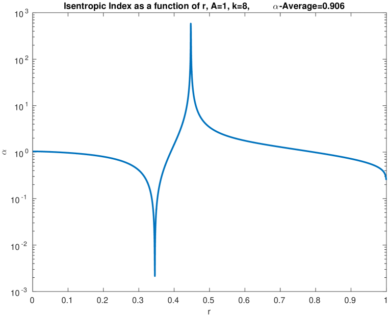
Figure 1:

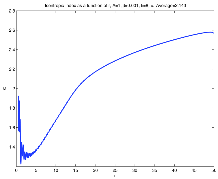
Figure 2:

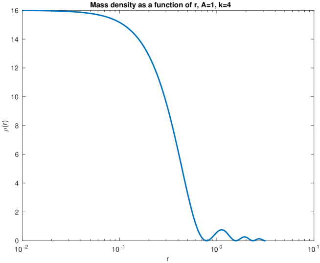
Figure 3:

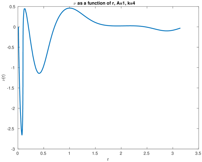
Figure 4:

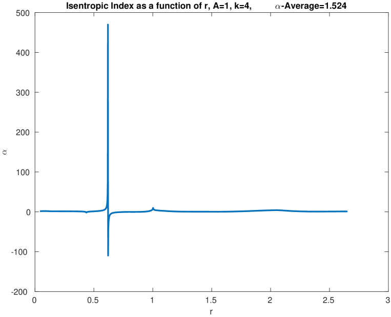
Figure 5:

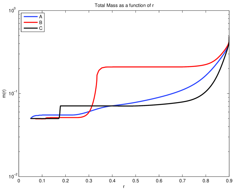
Figure 6:

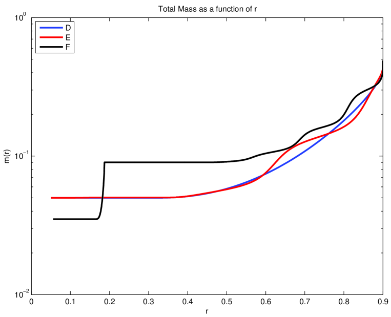
Figure 7:

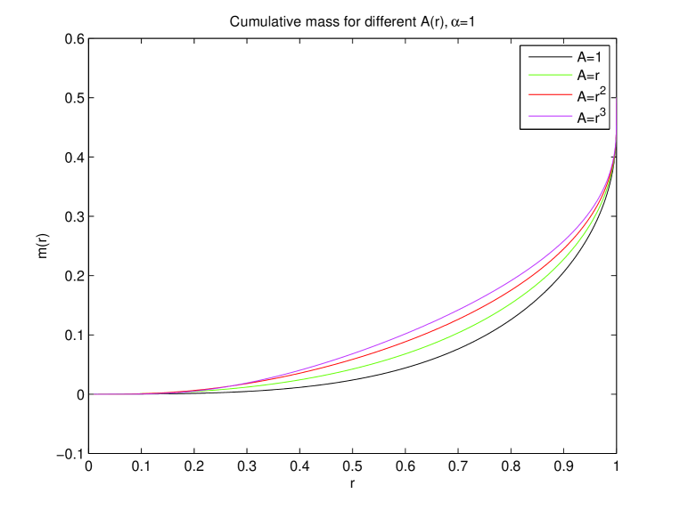
Figure 8:

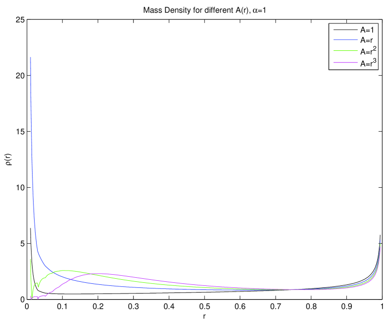
Figure 9:

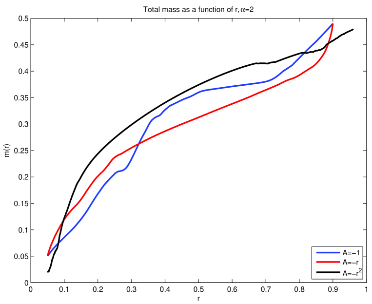
Figure 10:

References

- [1] J. L. Synge, Relativity, The General Theory (North Holland Publishing Co Amsterdam) (1960)
- [2] R. Adler, M. Bazin and M. Schiffer, Introduction to General Relativity, 2nd Edition McGraw-Hill Book CO. 1975.
- [3] J.B. Griffiths and J. Podolski, Exact Space-Times in Einstein’s General Relativity, Camb. Univ. Press 2009
- [4] Schwarzschild, K. (1916) Uber das Gravitationsfeld eines Massenpunktes nach der Einsteinschen Theorie, Sitzungsberichte der Koniglich Preussischen Akademie der Wissenschaften 7,189-196.
- [5] H. Weyl, Ann. Physik 54, 117 (1918);ibid, 59, 185 (1919);
- [6] T. Levi-Civita, Atti Accad. Naz. Lincei Rend. , Classe Sci. Fis. , Mat. e Nat bf 28 101 (1919)
- [7] R.C. Tolman, Static Solutions of Einstein field equations for Spheres of fluids, Phys. Rev. 55 p.364 (1939)
- [8] J. Robert Oppenheimer and George Volkoff, On Massive Neutron Cores, Phys. Rev 55 374-381, 1939
- [9] H. A. Buchdahl, General relativistic fluid spheres, Phys. Rev. 116 (1959), 1027.
- [10] R.J. Adler, A fluid Sphere in General Relativity, J. Math. Phys. 15 727 (1974)
- [11] M. Woolfson, The origin and evolution of the solar system, Astronomy & Geophysics. 41 (1): 12.
- [12] Matsumoto, T. and Hanawa T., 1999 Bar and Disk Formation in Gravitationally Collapsing Clouds. Astrophys. J., 521(2), pp.659-670
- [13] M. Arik, O.Delice, Static cylindrical matter shells, Gen. Rel. Grav. 37, p.1395-1403 (2005)
- [14] L. Herrera, A. Di Prisco, J. Iba?ez, J. Ospino, Axially symmetric static sources: A general framework and some analytical solutions, Phys. Rev. D87, 024014-10, (2013)
- [15] S. S. Bayin, Anisotropic fluid spheres in general relativity, Phys. Rev. D 26 (1982), 1262.
- [16] S. K. M Aurya , Y. K. Gupta and M. K. Jasim, Relativistic Modeling of Stable Anisotropic Super-Dense Star, Reports on Mathematical Physics, 76(2015) 21-40
- [17] M. Humi, J.A. LeBritton, Interior solutions to plane symmetric Einstein-Maxwell Equations. Phys. Rev. D II p. 2689 (1975).
- [18] M. Humi, J. Mansour - Interior Solutions to Einstein-Maxwell equations, Phys. Rev. D. 29 p. 1076 (1984).
- [19] N. Van den Bergh and R. Slobodeanu - Shear-free perfect fluids with a barotropic equation of state in general relativity: the present status, Class. Quantum Grav. 33 085008 (2016)