Noise-induced standing waves in oscillatory systems with time-delayed feedback

Abstract

In oscillatory reaction-diffusion systems, time-delay feedback can lead to the instability of uniform oscillations with respect to formation of standing waves. Here, we investigate how the presence of additive, Gaussian white noise can induce the appearance of standing waves. Combining analytical solutions of the model with spatio-temporal simulations, we find that noise can promote standing waves in regimes where the deterministic uniform oscillatory modes are stabilized. As the deterministic phase boundary is approached, the spatio-temporal correlations become stronger, such that even small noise can induce standing waves in this parameter regime. With larger noise strengths, standing waves could be induced at finite distances from the (deterministic) phase boundary. The overall dynamics is defined through the interplay of noisy forcing with the inherent reaction-diffusion dynamics.

I Introduction

Reaction-diffusion models define a paradigmatic class of systems to study wave patterns in spatially-extended media far from thermal equilibrium Hoyle06 . Beyond their natural use in chemical systems Kapral95 , they have been applied to general pattern-forming dynamical systems CrossRMP93 , kinetic roughening systems Halpin-Healy95 , biological systems Murray89 , among others.

Here, we consider the case where the reaction-diffusion system has undergone a smooth transition from a stationary state to uniform oscillations, a scenario captured by the supercritical Hopf bifurcation. The temporal and spatio-temporal behavior of the system is then described by the complex Ginzburg-Landau equation (CGLE) CrossRMP93 . However, uniform oscillations are not the only solution to that equation: among the most studied traveling wave solutions are one-dimensional plane waves and two-dimensional spiral waves. Furthermore, fascinating aspects of such dynamics concern unstable oscillations often leading to spatio-temporal chaos, like phase turbulence and defect chaos Murray89 ; AransonRMP02 ; PeregoPRL16 . The motivation of our work is to suppress spatio-temporal chaos in the CGLE and to replace it with regular patterns in a stochastically forced setting. The underlying method with which we achieve this is time-delay feedback.

Control of chaotic states in pattern-forming systems is a wide field of research that has already been reviewed in detail (e.g., in MikhailovPR06 ; Scholl07 ). In the context of the reaction-diffusion systems, the introduction of forcing terms or global feedback terms have been shown to be efficient ways to control turbulence. To cite just one example, chemical turbulence can be suppressed by global time-delayed feedback KimS01 ; BetaPRE03 in the CO oxidation reaction on Pt(110). In principle, most real physical feedbacks would need some time to influence the system. Although there may be cases where the feedback is fast enough compared to the intrinsic characteristic time scale and hence can be regarded as instantaneous, in general such a feedback would act with a time delay $\tau$. This sort of delay may appear under two heads, a spatially dependent local feedback and a spatially independent global feedback. In global feedback, a spatially-averaged variable or a variable without space dependence is fed back to the system dynamics. In the context of the CGLE, global feedback with explicit time delay was considered by Battogtokh and Mikhailov BattogtokhPD96 and then Beta and Mikhailov BetaPD04 . The latter used the Pyragas feedback scheme, where the feedback signal is created from the difference between the actual system state and a time-delayed one PyragasPLA92 . Among other features, the authors reported a parameter regime between spatio-temporal chaos and uniform oscillations where standing wave patterns were observed.

The presence of noise changes the dynamics of nonlinear, spatially-extended systems significantly, as noise can not only destabilize certain patterns, but it also can enhance and induce others, as reviewed in GarciaOjalvo99 . Recently, the effect of noise on systems subjected to time delay has attracted interest, like in the context of noise-induced oscillations PomplunEpL05 , correlation times BrandstetterPTRSA10 , stochastic bifurcation ZakharovaPRE10 , coherence resonance GeffertEPJB14 , stochastic switching DhuysPRE14 , or autonomous learning KaluzaPRE14 . These studies, though, primarily focus on systems without spatial extension, whereas this article considers a reaction-diffusion system and therefore enables us to study a spatially-extended wave pattern under the simultaneous influence of time delay and noise. In the context of extended systems, different features of spatial and temporal coherence due to noise (but without time delay) close to pattern-forming instabilities CarrilloEpL04 , in excitable systems PercPRE05 , and for coupled chaotic oscillators ZhouPRE02 ; KissC03 have been considered. The effect of noise on time-delay models has been studied, e.g., for a network of excitable Hodgkin-Huxley elements WangPLA08 .

This work builds on the foundation laid out in the seminal work by DeDominicis and Martin DeDominicis79 ; Chattopadhyay01 . Based on a stochastically forced Burgers’ dynamics, later to be followed by the paradigmatic Kardar-Parisi-Zhang model Kardar86 , the results highlighted the importance of stochastic forcing in second order phase transitions Barabasi95 . Here we take this approach one step further, by including a finite time delay in a stochastically forced spatio-temporal dynamics that threads together vital “missing links” in the causality analysis of a perturbed stochastic dynamics. The key construct here is the segregation of the mean and fluctuating components of a dynamical field, in line with the DeDominicis-Martin scheme DeDominicis79 . The methodology has recently been successfully used in fluid and magnetohydrodynamic models as well Chattopadhyay01 ; Chattopadhyay13 ; Chattopadhyay14 . In this approach, each vector field $\phi$ will be split into a mean component $\phi_{0}$ and a stochastic random part $\delta\phi$ representing the (often) nonlinear flow close to the boundary layer as follows: $\phi=\phi_{0}+\delta\phi$. The component $\delta\phi$ represents the fluctuation dominated regime away from the line of symmetry. Such a segregation of deterministic and stochastic components in the model allows one to study the perturbed dynamics of $\delta\phi$ around the mean (symmetry) variable $\phi_{0}$ as a set of two coupled equations, one in $\delta\phi$ and the other in $\phi_{0}$.

The focal point here is the analysis of the above stochastically forced dynamical field $\delta\phi$ in the context of time delay. In a series of works BetaPD04 ; StichPRE07 ; StichPD10 ; StichPRE13 , time-delay feedback has been used to suppress spatio-temporal chaos in the CGLE without stochastic terms and different aspects have been considered, like the interplay of local vs. global feeback terms StichPRE07 , the stability of the uniform solutions StichPD10 , and the standing-wave solution StichPRE13 . In this work, instead of including local feedback terms, for the sake of simplicity we use a stochastic generalization of the model with purely global feedback, introduced in Ref. BetaPD04 . In the context of our model, our interests are in understanding the following: a) how noise modifies the transition from a turbulent regime via standing waves to a state of uniform oscillations, and b) whether standing waves themselves can be induced by noise.

This paper is organized as follows: in Section II, we introduce the model and describe briefly the relevant deterministic solutions, uniform oscillations and standing waves. In Section III, we introduce noise terms and calculate the spatio-temporal correlation functions. In Section IV, we show numeric simulations to explore the onset of standing waves in the presence of noise. A summary of results and future directions of research are presented in Section V.

II The deterministic model and its main solutions

Reaction-diffusion systems can display various types of oscillatory dynamics. However, close to a supercritical Hopf bifurcation, all such systems are described by the complex Ginzburg-Landau equation (CGLE) CrossRMP93 ,

$$\frac{\partial A(x,t)}{\partial t}=(1-{\rm i}\omega)A-(1+{\rm i}\alpha)|A|^{2}A+(1+{\rm i}\beta)\Delta A,$$ (1)

where $A$ is the complex oscillation amplitude, $\omega$ the linear frequency parameter, $\alpha$ the nonlinear frequency parameter, $\beta$ the linear dispersion coefficient, and $\Delta$ stands for the Laplacian operator. For $1+\alpha\beta<0$ (the Benjamin-Feir-Newell criterion), uniform oscillations $A_{u}={\mathrm{exp}}(-{\mathrm{i}}(\omega+\alpha)t)$ are unstable and spatio-temporal chaos is observed. In analogy with DeDominicis79 , the $\phi_{0}$ there serves the role of the spatio-temporal field variable $A(x,t)$.

The CGLE for a one-dimensional medium with global time-delayed feedback $F$ has been introduced in Ref. BetaPD04 and is defined by

$$\frac{\partial A(x,t)}{\partial t} = (1-{\rm i}\omega)A-(1+{\rm i}\alpha)|A|^{2}A$$ (2a)

$$+ (1+{\rm i}\beta)\frac{\partial^{2}A}{\partial x^{2}}+F,\>\>\text{and}$$

$$F=\mu{\mathrm{e}}^{{\mathrm{i}}\xi}\left(\bar{A}(t-\tau)-\bar{A}(t)\right),$$ (2b)

where $\bar{A}(t)=\frac{1}{L}\int_{0}^{L}A(x,t)\,{\rm d}x$ denotes the spatial average of $A(x,t)$ over a one-dimensional medium of length $L$. The parameter $\mu$ describes the feedback strength and $\xi$ characterizes a phase shift between the feedback and the current dynamics of the system.

The solution of the feedback-induced uniform oscillations is given by $A_{UO}(t)=\rho_{0}{\mathrm{exp}}(-{\mathrm{i}}\Omega t)$ BetaPD04 , where the amplitude and frequency are given by

$$\rho_{0} = \sqrt{1+\mu[\cos(\xi+\Omega\tau)-\cos\xi]},$$ (3a)

$$\Omega = \omega+\alpha+\mu\bigg{[}\alpha(\cos(\xi+\Omega\tau)-\cos\xi)$$ (3b)

$$- (\sin(\xi+\Omega\tau)-\sin\xi)\bigg{]}\,.$$

In general, no explicit analytic solution for Eqs. (3) can be given. Nevertheless, the solutions can be found numerically using root-finding algorithms. In order to understand the suppression of spatio-temporal chaos, a linear stability analysis for uniform oscillations was done BetaPD04 . At stable uniform oscillations, control of chaos was consistently achieved. Obviously, this depends not only on the CGLE parameters, but also on the control parameters, in particular $\mu$ and $\tau$ (we consider a fixed $\xi$ throughout the article). In the limits where the feedback strength or the time delay go to zero, the feedback term also goes to zero. This makes the scheme ineffective, and spatio-temporal chaos is recovered.

In order to analyze the stochastically forced CGLE model, the stability boundaries of uniform oscillations in the parameter space need to be ascertained for the deterministic model (2). These boundaries are given by the conditions $\lambda_{1}=0$ and $\partial_{p}\lambda_{1}\neq 0$, where $\lambda_{1}$ is thereal part of the dominant eigenvalue (the others must be negative) and $p$ stands for either $\mu$ or $\tau$. As shown in detail in BetaPD04 ; StichPD10 , we can specify the parameter sets for which the uniform periodic solution becomes unstable with respect to standing waves with wavelength $2\pi/k_{c}$ ($k_{c}\neq 0$), where $k_{c}$ is the critical wavenumber as given by the linear stability analysis of the uniform oscillations BetaPD04 . It varies between $0.7$ and $0.9$ for the parameter set we are interested in, see Fig. 5(b) of BetaPD04 .

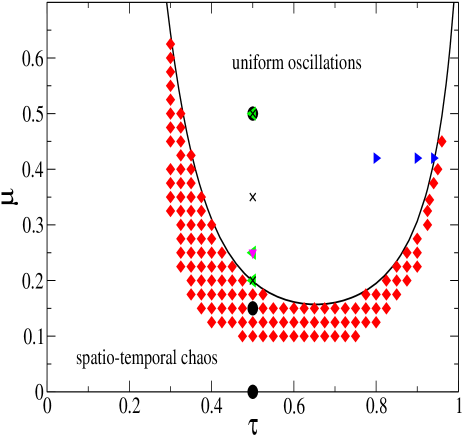
Figure 1: Main solutions in the parameter space spanned by $\tau$ and $\mu$. The solid line defines the stability boundary of uniform oscillations in the deterministic system (above the curve). Below that curve, the diamond symbols indicate simulations displaying standing waves in the deterministic system (data from Fig. 8 of Ref. BetaPD04 and own simulations). The circles denote the parameter values chosen as defined in Fig. 2, while the left triangles indicate the parameter values as used for Fig. 3(a,b); the right triangles represent the parameter values as used for Fig. 3(c,d), and the down triangle stands for the parameter value for Fig. 5. The crosses represent the parameter values used in Fig. 6. Note that with the exception of Fig. 2(b,c,d), all simulations were performed in the deterministically stable regime characterized by uniform oscillations where standing waves do not exist. The other parameters are: $\alpha=-1.4$, $\beta=2$, $\omega=2\pi-\alpha$, $\xi=\pi/2$.

In Fig. 1, a part of the $\mu-\tau$ parameter space is shown where uniform oscillations are stable (above the solid curve), and where standing waves are found numerically (diamonds). The other symbols indicate parameter values used in later figures.

Simulations confirm that the onset of standing waves is smooth, and that the standing wave is characterized by a vanishing space-dependent part at threshold. In this model, standing wave solutions are described by StichPRE13

$$A_{SW}={\mathrm{e}}^{-{\mathrm{i}}\Omega_{0}t}(H_{0}+2B_{k0}\cos(kx){\mathrm{e}}^{-{\mathrm{i}}\gamma}),$$ (4)

where $k$ is given by the eigenvalue problem studied in BetaPD04 , i.e., it corresponds either to $k_{c}$ (at onset of the standing wave pattern, $\lambda_{1}=0$) or $k_{max}$ (away from onset, $\lambda_{1}\neq 0$), and $H_{0}$, $B_{k0}$, $\Omega_{0}$, and $\gamma$ are given by a set of nonlinear equations given in StichPRE13 . This deterministic formulation will be later used as we define the amplitude of noise-induced standing waves.

Spatio-temporal simulations are performed for a one-dimensional system with size $L=256$ and spatial resolution $\Delta x=0.32$. For time integration, we use an explicit Euler scheme with $\Delta t=0.002$. The Laplacian operator is discretized using a next-neighbor representation, as discussed for the deterministic model used in StichPRE13 (and references therein). We apply periodic boundary conditions and the initial conditions consist of developed spatio-temporal chaos as present in the absence of feedback. Usually, the system settles to an asymptotic state before $t=200$, while we let it evolve until $t=500$. Then, we start the simulations that are shown in Figs. 1, 2, 5, 6.

In Fig. 2, we give an overview of the most relevant patterns, as observed in the simulations of the model defined in Eq. (2). The upper panels show space-time diagrams of $|A|$, the lower panels representing the solutions for the real part of the amplitude. The latter illustrates the oscillations, while the former reveal the amplitude of the oscillations and whether they have a space dependence. According to the Benjamin-Feir-Newell criterion, the Ginzburg-Landau parameters $\alpha$ and $\beta$ are chosen to fulfill $1+\alpha\beta<0$, i.e., in the absence of feedback, the system converges to the regime of spatio-temporal chaos. This is shown in space-time diagrams for $|A|$ and Re$A$ (Fig. 2(d)), where Re$A$ denotes the real part of $A$. But in the presence of strong feedback ($\mu=0.5$), the feedback induces uniform oscillations (Fig. 2(a)). For an appropriate choice of the delay time $\tau$, between the chaotic region and the region of uniform oscillations, standing waves are observed. As $\mu$ decreases (for this $\tau$, at $\mu_{c}=0.19848$), small-amplitude standing waves set in (Fig. 2(b)). These standing waves are spatial modulations of the underlying uniform oscillations. For comparison with the stochastic model discussed below (Section IV), we show in Fig. 2(c) the impact of small noise to the standing waves (otherwise same parameters as in Fig. 2(b)). If the noise is small enough, the observed pattern is stable and clearly recognizable, in spite of inevitable small fluctuations.

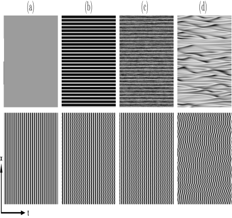
Figure 2: Main spatio-temporal solutions for different feedback magnitudes and noise strengths: (a) uniform oscillations, (b) standing waves without noise, (c) standing waves with small noise, (d) spatio-temporal chaos. Shown are space-time diagrams in gray scale for $|A|$ (top panels) and Re$A$ (bottom panels) for a time interval of $t=25$ in the asymptotic regime and system size $L=256$. The delay time is $\tau=0.5$ and the values of $\mu$ are $\mu=0.50$ (a), $\mu=0.15$ (b), $\mu=0.15$ (c), $\mu=0$ (d). The noise magnitude is $D=0.05$ in (c) and zero otherwise. Black (white) denotes low (high) values of the respective quantity (rescaled for each simulation). For $|A|$, these values are $(|A|_{min},|A|_{max})=(0.94,1.13)$ (b), $(|A|_{min},|A|_{max})=(0.9,1.15)$ (c), $(|A|_{min},|A|_{max})=(0.15,1.2)$ (d). For (a), the amplitude is constant $|A|=1.085$. The other parameters are as in Fig. 1.

III The stochastic model and its correlation functions

While previous works BetaPD04 ; StichPRE13 gave us an understanding of standing waves in the deterministic system, the dynamics of these waves in the presence of noise and in particular their onset are unknown. In order to tackle this question, we analyze the stochastic Langevin model, starting from equations (2). This can be accomplished by studying the impact that the spatio-temporal noise $N(x,t)$ has on the system, in particular when we approach the instability of uniform oscillations with respect to perturbations with $k\neq 0$. Model (2) therefore becomes

$$\frac{\partial A}{\partial t} = (1-{\rm i}\omega)A-(1+{\rm i}\alpha)|A|^{2}A$$ (5a)

$$+ (1+{\rm i}\beta)\frac{\partial^{2}A}{\partial x^{2}}+F+N(x,t),$$

$$\langle N(x,t)N(x^{\prime},t^{\prime})\rangle = 2D\delta(x-x^{\prime})\delta(t-t^{\prime}),$$ (5b)

where $N(x,t)$ stands for a Gaussian, white noise with magnitude $D$, and where $F$ is given in Eq. (2b). In order to calculate the correlation functions, we resort to a Fourier series expansion of $N(x,t)$ as follows

$$N(x,t)=\int\tilde{N}_{k,\tilde{\omega}}\,{\mathrm{e}}^{{\mathrm{i}}(kx-\tilde{\omega}t)}{\mathrm{d}}k\,{\mathrm{d}}\tilde{\omega}.$$ (6)

For $A$, we use the ansatz

$$A(x,t)=\rho_{0}\exp(-{\mathrm{i}}\Omega t)+A_{+}\exp({\mathrm{i}}kx)+A_{-}\exp(-{\mathrm{i}}kx),$$ (7)

where $A_{\pm}$ represent the amplitudes of the linearly independent solutions $\exp(\pm{\mathrm{i}}kx)$, phenomenologically representing oppositely directed waves from left to right or from right to left. The wave vector $k$ is determined from linear stability analysis, details of which are available in BetaPD04 . Our interest is in the spatio-temporal autocorrelations of the field $A$ that will allow us to compare and establish the contributions from stochasticity driven perturbations against the results obtained in the previous non-noisy cases BetaPD04 ; StichPRE07 ; StichPD10 . The necessary quantities to calculate in this connection are respectively the autocorrelation function $C_{0}=\langle A(x,t)*A^{*}(x,t)\rangle$, the spatial correlation function $C_{r}=\langle{[A^{*}(x+r,t)-A(x,t)]}^{2}\rangle=2(C_{0}-\langle A^{*}(x+r,t)*A(x,t)\rangle)$ and the temporal correlation function $C_{t^{\prime}}=\langle{[A^{*}(x,t+t^{\prime})-A(x,t)]}^{2}\rangle=2(C_{0}-\langle A^{*}(x,t+t^{\prime})*A(x,t)\rangle)$. The brackets denote ensemble averages. Straightforward algebra then leads us to the following results:

$$C_{0} = 2D\bigg{[}{|\rho_{0}|}^{2}xt+\frac{4}{k(\lambda_{1}^{2}+\lambda_{2}^{2})}\text{Re}(\rho_{0}{A_{+}}^{*(0)}+\rho_{0}{A_{-}}^{*(0)})$$ (8a)

$$\times \sin\left(\frac{kx}{2}\right)\bigg{[}{\mathrm{e}}^{\lambda_{1}t}\left(\lambda_{1}\cos(\lambda_{2}t+\frac{kx}{2})+\lambda_{2}\sin(\lambda_{2}t+\frac{kx}{2})\right)$$

$$- \lambda_{1}\cos(\frac{kx}{2})-\lambda_{2}\sin(\frac{kx}{2})\big{]}\bigg{]}$$

$$C_{r} = \frac{8D}{k({\lambda_{1}}^{2}+{\lambda_{2}}^{2})}\bigg{[}\text{Re}(\rho_{0}{A_{+}}^{*(0)}+\rho_{0}{A_{-}}^{*(0)})e^{\lambda_{1}t}\big{[}\sin(\frac{kx}{2})$$ (8b)

$$\times (\lambda_{1}\cos(\lambda_{2}t+\frac{kx}{2})+\lambda_{2}\sin(\lambda_{2}t+\frac{kx}{2}))-\sin(\frac{k}{2}(x+r))$$

$$\times (\lambda_{1}\cos(\lambda_{2}t+\frac{k}{2}(x+r))+\lambda_{2}\sin(\lambda_{2}t+\frac{k}{2}(x+r)))\big{]}$$

$$\times \lambda_{1}[\cos(\frac{kx}{2})-\cos(\frac{k}{2}(x+r))]$$

$$+ \lambda_{2}[\sin(\frac{kx}{2})-\sin(\frac{k}{2}(x+r))]\bigg{]}$$

$$C_{t^{\prime}} = 2\bigg{[}C_{0}-2D{\mathrm{e}}^{{\mathrm{i}}\Omega t^{\prime}}\big{[}{|\rho_{0}|}^{2}xt+{\rho_{0}}^{*}A_{+}^{(0)}\left(\frac{1-{\mathrm{e}}^{{\mathrm{i}}kx}}{{\mathrm{i}}k\lambda}\right)\left(1-{\mathrm{e}}^{\lambda t}\right)$$ (8c)

$$- {\rho_{0}}^{*}A_{-}^{(0)}\left(\frac{1-{\mathrm{e}}^{-{\mathrm{i}}kx}}{{\mathrm{i}}k\lambda^{*}}\right)\left(1-{\mathrm{e}}^{\lambda^{*}t}\right)$$

$$- {\rho_{0}}{A_{+}}^{*(0)}\left(\frac{1-{\mathrm{e}}^{-{\mathrm{i}}kx}}{{\mathrm{i}}k\lambda^{*}}\right)\left(1-{\mathrm{e}}^{\lambda^{*}t}\right)$$

$$+ {\rho_{0}}{A_{-}}^{*(0)}{\mathrm{e}}^{\lambda t^{\prime}}\left(\frac{1-{\mathrm{e}}^{{\mathrm{i}}kx}}{{\mathrm{i}}k\lambda}\right)\left(1-{\mathrm{e}}^{\lambda t}\right)\big{]}\bigg{]},$$

where $\lambda=\lambda_{1}+{\mathrm{i}}\lambda_{2}$ and $\lambda^{*}=\lambda_{1}-{\mathrm{i}}\lambda_{2}$, $\lambda_{1,2}$ being the solutions of the quadratic equation $\lambda^{2}-2(1-k^{2}{\rho_{0}}^{2})\lambda+[1+\omega^{2}+2\beta\omega k^{2}+4\alpha\omega{\rho_{0}}^{2}+(1+\beta^{2})k^{4}+4\alpha\beta{\rho_{0}}^{2}k^{2}+3(1+\alpha^{2}){\rho_{0}}^{4}]=0$ (see Ref. BetaPD04 ) and $\rho_{0}$ and $\Omega$ are given by Eqs. (3). Note that $\lambda_{1}$ denotes here the real parts of the eigenvalues of the linear stability analysis of uniform oscillations, as explained above.

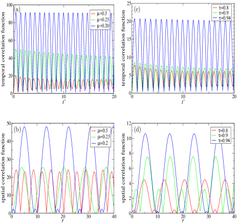
Figure 3: (a,b) Amplitudes of temporal (a) and spatial (b) correlation functions for $\tau=0.5$ for three different values of $\mu$ (see legend) and $D=1$. We observe that the closer $\mu$ to the critical $\mu_{c}=0.19848$, the larger the magnitude of the correlation functions. For illustration, we rescale (multiply) the temporal correlation functions with 1000 ($\mu=0.5$) and 50 ($\mu=0.25$) and the spatial correlation functions with 100 ($\mu=0.5$) and 50 ($\mu=0.25$). (c,d) Amplitudes of temporal (c) and spatial (c) correlation functions for $\mu=0.42$ for three different values of $\tau$ (see legend) and $D=1$. We observe that the closer $\tau$ to the critical $\tau_{c}=0.94244$, the larger the magnitude of the correlation functions. For illustration, we rescale (multiply) the correlation functions with 10 ($\tau=0.8$) and 5 ($\tau=0.9$). All other parameters are as in Fig. 1.

In this context, spatial and temporal correlation functions are of particular interest. In Fig. 3(a,b), we observe the amplitude of the spatial ($C_{r}$) and temporal ($C_{t^{\prime}}$) correlation functions for a fixed $\tau$ as we approach the instability of uniform oscillations and the simultaneous onset of standing waves (at $\mu_{c}=0.19848$). The influence of the noise can be expected to be more prominent as we approach the instability and hence the magnitude of the correlation functions should increase towards the instability. This is exactly what is observed in Fig. 3(a,b) for three different parameter values. To show different evaluations of the correlation functions in the same figure, we have rescaled the correlation functions (see figure captions). Since the solution describes temporal oscillations, they are also present in the temporal correlation functions (Fig. 3(a)). We see that away from the instability ($\mu=0.5$), the temporal correlation function approaches a constant envelope value after approximately 20 time units. On the other hand, the spatial correlation function (Fig. 3(b)) does not show a decaying property as the temporal one, and the periodicity corresponds to the $k$ value resulting from the linear stability analysis BetaPD04 .

In Fig. 3(c,d), we show the correlation functions (as functions of $r$ and $t^{\prime}$ respectively) for three values of $\tau$ while keeping $\mu=0.42$ constant. Qualitatively, we observe a similar behavior as in Fig. 3(a,b). As the delay time $\tau$ increases towards its critical value, the amplitude of the correlation functions also increases.

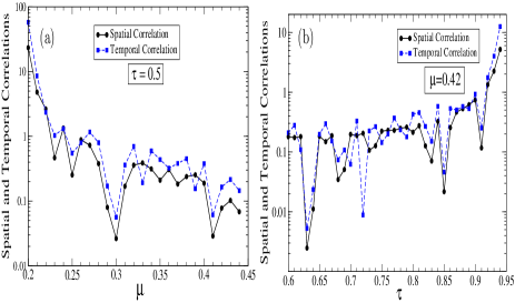
Figure 4: Amplitudes of temporal and spatial correlation functions for $\mu=0.42$ as $\tau$ is varied (a) and for $\tau=0.5$ as $\mu$ is varied (b). This figure complements the data shown in Fig. 3. To quantify the oscillating amplitudes, we choose the average value of the amplitude in one period within the asymptotic regime for large $t^{\prime}$ and $r$. As $\mu$ is varied in (a), the amplitude of the correlation functions is low in the area of deterministically stable oscillations, but increases towards the limits of the stability region. As $\tau$ is varied in (b), we observe qualitatively similar behavior: here the uniform oscillations lose stability as $\tau$ is lowered. The other parameters are as in Fig. 3.

In order to obtain a more complete picture of the spatial and temporal correlations, in Fig. 4, we vary $\tau$ in small steps for a fixed $\mu$ and vice versa. We have seen in Fig. 3 that as we approach the stability boundary, the amplitude of the correlation functions increases. For the temporal correlation function, we average over the time interval $[(30-2\pi/\Omega),30]$, and for the spatial correlation function, over the space interval $[(50-2\pi/k),50]$, in order to ensure ergodicity over one full period. As introduced above, $k$ denotes the most unstable wavenumber of the uniform oscillations, and $\Omega$ their frequency. Figure 4 shows that indeed the correlation functions increase towards to the boundary where uniform oscillations cease to be stable and standing waves set in the deterministic system.

IV Spatio-temporal simulations in the presence of noise and feedback

The expressions given in equations (8b) and (8c) can be interpreted as a linear superposition of two waves at the phase points $(k,x)$ and $(k,x+r)$ for all time points, and with the same amplitude which is proportional to the noise strength $D$. In other words, our model solution of the correlation functions lead to noise-induced standing waves. In this section, we show simulations that corroborate this. The amplitude of the Gaussian noise term scales as $1/\sqrt{\Delta x\Delta t}$. This happens because the two-point noise correlation is proportional to $\delta(x-x^{\prime})\delta(t-t^{\prime})$. In the Euler discretization scheme, the additive noise scales as $\sqrt{\Delta t}$.

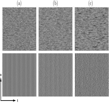
Figure 5: Spatio-temporal simulations for different values of $D$ and fixed feedback strength. In space-time plots, we show $|A|$ (upper panels) and $ReA$ (lower panels) for $D=0.05$ (a), $D=0.2$ (b) and $D=0.5$ (c). The feedback magnitude is $\mu=0.25$, the delay time $\tau=0.5$, and the other parameters are as in Fig. 1. For low $D$, we see that although $|A|$ shows some intermittent spatially periodic patches, their amplitude is actually quite small and the pattern actually is indistinguishable from uniform oscillations. For intermediate $D$, intermittent spatially periodic patches are seen in the pattern, reminiscent of standing waves. For large $D$, the noise is too strong to induce standing waves and the pattern corresponds to noisy uniform oscillations.

First, we consider a parameter value for which the deterministic solution corresponds to uniform oscillations: delay time is fixed to $\tau=0.5$ as above, and the feedback to $\mu=0.25$ which is larger than the critical one, $\mu_{c}=0.19848$. In Fig. 5, we show three simulations, for increasing noise strengths. For $D=0.05$ (a) we see an oscillatory pattern in the lower panel which is almost indistinguishable from uniform oscillations. However, the upper panel reveals that there is actually a spatial periodicity in $|A|$ and that this periodicity is temporally persistent over multiple oscillations. In the space-time plot, this is seen as patches of horizontal stripes. This means that we observe a noise-induced spatial pattern modulating the uniform oscillations, i.e., the formation of a standing wave pattern. This finding resembles spatial coherence CarrilloEpL04 , as we will comment on below.

If the noise intensity is increased to $D=0.2$ (panel (b) of Fig. 5), we see similar patches of horizontal stripes in the panel for $|A|$. However, their amplitudes are larger and therefore, this time there is also a visible modulation of the oscillatory pattern itself (lower panel of (b)). Hence, this pattern corresponds to noise-induced standing waves. It is important to note that the wavelength of the pattern corresponds to the wavelength predicted through the linear stability analysis shown in BetaPD04 ; StichPD10 . This means, the wavenumber $k$ corresponds to the wavenumber $k_{max}$ for which $\lambda_{1}$ reaches its maximum, while $\lambda_{1}(k_{max})<0$. If the noise intensity is increased further to $D=0.5$ (c), patches of stripes give rise to more irregular patches (upper panel). The lower panel shows oscillations that are now visibly distorted by the noise, but without any spatial periodicity.

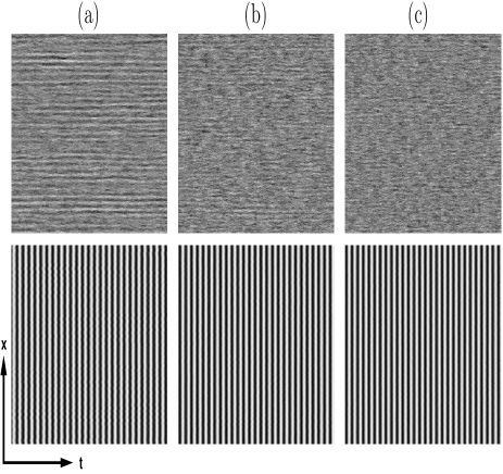
Figure 6: Spatio-temporal simulations for different values of $\mu$ and fixed noise. In space-time plots, we show $|A|$ (upper panels) and $ReA$ (lower panels) for $\mu=0.2$ (a), $\mu=0.35$ (b) and $\mu=0.5$ (c). The noise strength is $D=0.05$, the delay time $\tau=0.5$, and the other parameters are as in Fig. 1. For low $\mu$, we observe clearly spatially periodic patterns that correspond to noise-induced standing waves. For larger $\mu$ (and hence further from the deterministic onset of standing waves), standing waves are weaker. For high $\mu$, the noise is not enough to induce standing waves.

We can now fix the noise intensity and explore the effect of varying the feedback magnitude. In Fig. 6, using $D=0.05$, we display the results of spatio-temporal simulations for three values of $\mu$ that all correspond to the regime where no standing waves are stable in the deterministic system. First, we fix $\mu=0.2$ (a), a value that ensures closeness to the onset of the standing wave regime. Not surprisingly, we therefore see clear indication of standing waves in the panel for $|A|$. However, similar to what has been shown in Fig. 6(a), the pattern amplitude is not large enough compared to the uniform mode to be clearly seen in the oscillations (lower panel). Increasing the feedback magnitude to $\mu=0.35$ (b), we see only weak evidence for patches of standing waves (upper panel), and moving even further from the stability boundary ($\mu=0.5$ in (c)), standing waves cannot be induced by weak noise.

To assess the onset of noise-induced standing waves in more detail, we obtain from the simulations (Figs. 5 and 6) the amplitude of the standing waves. To be precise, we show its spatial contribution $2B_{k0}$ (see Eq. (4)), which should be compared to the uniform contribution $H_{0}$, of order unity. Due to the noisy character of the simulations, the standing waves occur only intermittently and it is difficult to obtain their amplitude. In Fig. 7, we show how this amplitude varies with $D$ for fixed $\tau$ and $\mu$ (a) and with $\mu$ for fixed $\tau$ and $D$ (b).

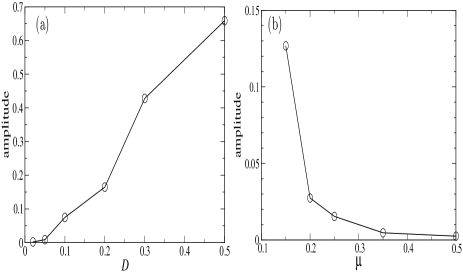
Figure 7: Amplitude of noise-induced standing waves. In (a), this amplitude is shown as a function of the noise strength $D$ for a fixed set of $\tau=0.5$ and $\mu=0.25$. As qualitatively seen in Fig. 5, for small $D$ the amplitude is very small and not perceivable, for intermediate $D$ the amplitude is large and visible, while for large noise strengths, the overall pattern becomes too irregular to actually identify standing waves. In panel (b), the amplitude of standing waves is shown as a function of the feedback strength $\mu$ for a fixed set of $\tau=0.5$ and noise strength $D=0.05$. The leftmost point ($\mu=0.15$) corresponds to deterministically stable standing waves with relatively large amplitude. Starting from $\mu=0.2$, we enter the regime where standing waves do not exist as deterministic solutions, and we see that the amplitude diminishes as we move away from the stability coundary of uniform oscillations. The other parameters are as in Fig. 1.

As seen in Fig. 7(a), the amplitude increases monotonically with $D$. The standing waves identified in the simulations are in the intermediate parameter range: for small $D$, uniform oscillations dominate, and for large $D$, the pattern becomes very noisy on the background of uniform oscillations. In the scenario shown in Fig. 7(b), we observe a monotonically decreasing amplitude profile with increasing $\mu$ that indicates damping of the noise at large feedbacks. As we deviate more and more from the stability boundary, a given noise $D=0.05$ becomes more and more ineffective to induce standing waves. Note that the first data point ($\mu=0.15$) is already in the regime of deterministically stable standing waves.

V Conclusion

In this article, we studied standing waves for a complex Ginzburg-Landau equation (CGLE) in the presence of global time-delay feedback and noise and studied their properties analytically and numerically. The CGLE describes the dynamics of a spatially-extended system that undergoes a supercritical Hopf bifurcation. The basic solution in this system corresponds to uniform oscillations. We considered the situation where this solution is Benjamin-Feir unstable in the absence of feedback ($1+\alpha\beta<0$), leading to spatio-temporal chaos. Then, uniform oscillations or standing waves can be induced through the time-delay feedback. Standing waves can be understood as instability of the uniform oscillations, namely when the oscillations become unstable with respect to perturbations with a certain wavenumber (shown in Fig. 2(b)). These waves represent a transition state between uniform oscillations and a chaotic state.

One main finding is that noise can induce standing waves in the regime where uniform oscillations are stable (Figs. 5 and 6). The closer we are to the stability boundary that separates uniform oscillations and standing waves, the less noise intensity is needed to induce standing waves. If the system is at a finite distance from that boundary, a comparatively larger magnitude of the noise is needed to induce standing waves. In the limit $D\to 0$, no standing waves can be expected. However, as $D$ becomes large, rather than inducing standing waves, irregular uniform oscillations are observed. Hence, intermediate noise magnitudes are favorable for the induction of standing waves. These results are similar in spirit with findings of spatial or spatio-temporal coherence resonance (e.g., CarrilloEpL04 ; PercPRE05 ; ZhouPRE02 ). In contrast to those works, however, we consider a system where the stable noise-free state consists of uniform oscillations and the stabilized noise-induced pattern consists of standing waves. The wavenumber of the induced standing waves agrees qualitatively with the value of $k$ for the most unstable mode, as obtained by the stability analysis of uniform oscillations. This is a common feature with pattern-forming systems like the one discussed in CarrilloEpL04 due to the appearance of an intrinsic length scale.

For the noisy CGLE and in absence of feedback, standing waves have not been reported. So feedback is still essential for finding standing waves. However, we emphasize that the onset of standing waves can be controlled by noise. The CGLE represents an oscillatory reaction-diffusion system where the chaos is diffusion-induced and hence there is a fundamental difference to the oscillators in ZhouPRE02 ; KissC03 which display a chaotic dynamics without coupling and where phase synchronization of oscillations (and no standing waves) are observed.

The correlation functions evaluated in the regime of deterministically stable uniform oscillations (Fig. 3) show oscillations that increase while approaching the deterministic stability boundary, corroborating the idea of noise-induced standing waves in this parameter regime. More generally, we note that noise does not destroy the deterministic Hopf bifurcation structure itself but only modulates the instability leading to standing waves. We have verified this for the range of parameter values studied, i.e., for small delays $\tau\leq 1$ and moderate feedback magnitudes $\mu\leq 1$. Future work will target different (wider) regimes.

We showed that small noise does not destabilize deterministically stable standing waves (Fig. 2(c)), but we have not studied systematically what effect noise exerts on standing waves where these are stable in the deterministic system and on the chaotic solution itself. Future work may comprise a study to characterize these dynamics and separate it from spatio-temporal chaos that is found when the feedback strength is decreased in the deterministic system.

VI Acknowledgments

MS acknowledges stimulating discussions with Carsten Beta and Eckehard Schöll.

References

- (1) R. Hoyle, Pattern Formation: An Introduction to Methods (Cambridge Univ. Press, Cambridge, 2006).
- (2) Chemical Waves and Patterns, edited by R. Kapral and K. Showalter (Kluwer Academic, Dordrecht, 1995).
- (3) M. C. Cross and P. C. Hohenberg, Rev. Mod. Phys. 65, 851 (1993).
- (4) T. Halpin-Healy and Y.-C. Zheng, Phys. Rep. 254, 215 (1995).
- (5) J. D. Murray, Mathematical Biology (Springer, Berlin, 1989).
- (6) I. S. Aranson and L. Kramer, Rev. Mod. Phys. 74, 99 (2002).
- (7) A. M. Perego et al., Phys. Rev. Lett. 116, 028701 (2016).
- (8) A. S. Mikhailov and K. Showalter, Phys. Rep. 425, 79 (2006).
- (9) Handbook of Chaos Control, edited by E. Schöll and H. G. Schuster (Wiley-VCH, Weinheim, 2007).
- (10) M. Kim et al., Science 292, 1357 (2001).
- (11) C. Beta et al., Phys. Rev. E 67, 046224 (2003).
- (12) D. Battogtokh and A. Mikhailov, Physica D 90, 84 (1996).
- (13) C. Beta and A. S. Mikhailov, Physica D 199, 173 (2004).
- (14) K. Pyragas, Phys. Lett. A 170, 421 (1992).
- (15) J. García-Ojalvo and J. M. Sancho, Noise in spatially extended systems (Springer, New York, 1999).
- (16) J. Pomplun, A. Amann, and E. Schöll, Europhys. Lett. 71, 366 (2005).
- (17) S. Brandstetter, M. A. Dahlem, and E. Schöll, Phil. Trans. Roy. Soc. London A 368, 391 (2010).
- (18) A. Zakharova et al., Phys. Rev. E 81, 011106 (2010).
- (19) P. M. Geffert et al., Eur. Phys. J. B 87, 291 (2014).
- (20) O. D’Huys, T. Jüngling, and W. Kinzel, Phys. Rev. E 90, 032918 (2014).
- (21) P. Kaluza and A. S. Mikhailov, Phys. Rev. E 90, 030901(R) (2014).
- (22) O. Carrillo, M. A. Santos, J. Garcia-Ojalvo, and J. M. Sancho, Europhys. Lett. 65, 452 (2004).
- (23) M. Perc, Phys. Rev. E 72, 016207 (2005).
- (24) C. Zhou and J. Kurths, Phys. Rev. E 65, 040101(R) (2002).
- (25) I. Z. Kiss et al., Chaos 13, 267 (2003).
- (26) Q. Wang, M. Perc, Z. Duan, and G. Chen, Phys. Lett. A 372, 5681 (2008).
- (27) C. DeDominicis and P. C. Martin, Phys. Rev. A 19, 419 (1979).
- (28) A. K. Chattopadhyay and J. K. Bhattacharjee, Phys. Rev. E 63, 016306 (2001).
- (29) M. Kardar, G. Parisi, and Y. C. Zhang, Phys. Rev. Letts. 56, 889 (1986).
- (30) A. L. Barabasi and H. Stanley, Fractal Concepts in Surface Growth (Cambridge University Press, London, 1995).
- (31) B. Mukhopadhyay and A. K. Chattopadhyay, Phys. Rev. E 90, 063014 (2014).
- (32) S. K. Nath and A. K. Chattopadhyay, J. Phys. A 46, 035501 (2013).
- (33) M. Stich, A. C. Casal, and J. I. Díaz, Phys. Rev. E 76, 036209 (2007).
- (34) M. Stich and C. Beta, Physica D 239, 1681 (2010).
- (35) M. Stich, A. Casal, and C. Beta, Phys. Rev. E 88, 042910 (2013).