Screened exchange corrections to the random phase approximation from many-body perturbation theory

Abstract

The random phase approximation (RPA) systematically overestimates the magnitude of the correlation energy and generally underestimates cohesive energies. This originates in part from the complete lack of exchange terms, which would otherwise cancel Pauli exclusion principle violating (EPV) contributions. The uncanceled EPV contributions also manifest themselves in form of an unphysical negative pair density of spin-parallel electrons close to electron-electron coalescence.

We follow considerations of many-body perturbation theory to propose an exchange correction that corrects the largest set of EPV contributions while having the lowest possible computational complexity. The proposed method exchanges adjacent particle/hole pairs in the RPA diagrams, considerably improving the pair density of spin-parallel electrons close to coalescence in the uniform electron gas (UEG). The accuracy of the correlation energy is comparable to other variants of Second Order Screened Exchange (SOSEX) corrections although it is slightly more accurate for the spin-polarized UEG. Its computational complexity scales as $\mathcal{O}(N^{5})$ or $\mathcal{O}(N^{4})$ in orbital space or real space, respectively. Its memory requirement scales as $\mathcal{O}(N^{2})$.

1 Introduction

The random phase approximation (RPA) has become a widely used method for calculating total energies and other properties for extended systems in settings where the accuracy of the Hartree–Fock approximation or of density functional theory (DFT) is not sufficient. ¹ In such cases one can treat the electrostatic repulsion of the electrons among each other as a perturbation of the Hartree–Fock or DFT solution. The random phase approximation of the full many-body perturbation expansion consists of the infinite subset of terms where each perturbation interaction mediates the same momentum for all occurring states. The terms are called direct ring terms owing to their representation in form of Feynman diagrams. It was first introduced by Macke² to cure infinite energies occurring in finite order perturbation theories in metallic systems by summing over all orders of the perturbation before the summing over all occurring states — a procedure called resummation. Independently, RPA was also developed by Bohm and Pines³ from considerations on the polarizability. Owing to the ring structure of the expansion terms the random phase approximation can be calculated particularly efficiently. The two point polarizability is the only quantity that needs to be stored, such that the memory requirements of an RPA calculation scale as $\mathcal{O}(N^{2})$ with the number $N$ of electrons under consideration. Computation time scales as $\mathcal{O}(N^{6})$ solving the Casida equation, ^{4, 5} or as $\mathcal{O}(N^{5})$ solving the direct ring coupled cluster equations using a resolution of identity for the Coulomb integrals. ^{6, 7, 8} Employing numerical integration grids for imaginary time and imaginary frequency the complexity of the computation time is $\mathcal{O}(N^{4})$ in orbital space, and in real space even $\mathcal{O}(N^{3})$ can be achieved. ^{9, 10} Thus, in principle the complexity of an RPA calculation does not exceed that of a density functional theory calculation, the prefactor is however considerably larger.

Unfortunately, the random phase approximation does not approximate total energies in an unbiased way and in some situations hardly improves upon density functional theory. It consistently overestimates the magnitude of the (negative) correlation energy and tends to slightly underestimate cohesive energies and overestimate bond lengths as well as lattice constants. ^{11, 12, 13, 1, 6, 14, 15, 16, 17, 18} This is supposed to originate from contributions in the ring terms of the RPA that violate the Pauli exclusion principle, as outlined in more detail in Section 3. By the merit of Wick’s theorem such exclusion principle violating (EPV) contributions are exactly canceled by contributions in other terms of the exact many-body perturbation expansion where the offending states are exchanged.^{19, 20} Such expansion terms canceling EPV contributions of each other are called exchange terms.

The random phase approximation lacks exchange terms entirely. To correct for this deficiency a number of post-RPA approaches have been proposed and have been assessed for a range of systems.^{11, 21, 16} In direct ring coupled cluster doubles (drCCD) theory, the total energy can be calculated by anti-symmetrizing the final Coulomb interaction when tracing over the drCCD amplitudes. This approach offers a more balanced approximation to total correlation energies and some other properties but does not always improve energy differences. ^{7, 8, 6, 16} Compared to the direct RPA, the additional terms related to anti-symmetrization of the Coulomb interaction bear resemblance to a screened version of the second order Møller–Plesset exchange term and are therefore also referred to as second order screened exchange (SOSEX) terms. Computing drCCD is, however, more demanding, scaling as $\mathcal{O}(N^{5})$ in computation time and as $\mathcal{O}(N^{4})$ in memory, which often proves to be the limiting factor for extended systems. Even more types of exchange terms are incorporated in full coupled cluster singles and doubles (CCSD) theory. In fact, CCSD contains the largest set of terms that can be iteratively generated from two and four point quantities which is closed under including exchange terms, i.e. for each occurring term all its exchange terms are also included. Thus, CCSD fully respects the Pauli exclusion principle. It is, however, even more expensive with its computation time scaling as $\mathcal{O}(N^{6})$.

So far we have viewed the random phase approximation as an (infinite) subset of the many-body perturbation expansion, starting from either a Hartree–Fock, density functional theory (DFT) or a hybrid reference. The random phase approximation can also be derived using the adiabatic connection (AC) and the fluctuation dissipation theorem (FDT). In this context, the RPA total energy can be formulated in analogy to the direct term of second order Møller–Plesset (MP2) theory where one of the two interactions is screened and averaged over the AC interaction strength. Ángyán et al.²² suggested to add the exchange term of MP2 theory with the same coupling strength averaged screened interaction as an exchange correction to the RPA. This term is usually referred to as AC-SOSEX due to its resemblance to the SOSEX of drCCD. Although the AC-SOSEX cannot be formulated as a subset of the many-body perturbation expansion and, in fact, involves “inproper” vertices with two incoming or two outgoing arrows, it numerically yields very similar results as dr-CCD-SOSEX. In real space, its computation time scales as $\mathcal{O}(N^{4})$ with system size and its memory requirement only scales as $\mathcal{O}(N^{2})$ while that of drCCD-SOSEX scales as $\mathcal{O}(N^{4})$. The favorable scaling allows the application of AC-SOSEX to larger systems.

Rather than screening the interaction and using standard MP2, Bates et al.²³ propose an RPA-renormalized many-body perturbation theory in the adiabatic connection. Evaluating the second order exchange term within this theory gives the correction termed AXK, which improves on SOSEX and AC-SOSEX in chemical environments with static correlation. Other variants of screened exchange are discussed in Ref. 21.

Here, we propose an alternative ansatz for an exchange correction to the random phase approximation, which scales as favorably as AC-SOSEX, but which can also be formulated as an (infinite) subset of the many-body perturbation expansion, as drCCD-SOSEX can. Having a subset of the perturbation expansion one is again free to employ any reference theory of choice, such as Hartree–Fock or hybrid DFT functionals. MBPT also readily offers ground state expectation values, ^{24, 25} which can also be achieved in direct ring coupled cluster doubles by means of $\Lambda$-drCCD. ²⁶ We term the proposed exchange correction adjacent pairs exchange (APX) according to its diagrammatic representation.

1.1 Structure of this work

Section 2 briefly introduces the random phase approximation both, in terms of Feynman diagrams in the frequency domain, as well as in terms of Goldstone diagrams in the time domain. In Section 3 we define the terms of the adjacent pairs exchange correction from considerations on exclusion principle violating contributions in the RPA. Subsection 3.4 and 3.5 treat two other screened exchange variants and explains how APX differs from them.

In Section 4 we apply RPA+APX to the uniform electron gas (UEG) in the thermodynamic limit comparing total energies to two other SOSEX variants. Subsection 4.2 shows to what extent APX improves on the pair correlation function of the UEG, especially at the electron coalescence point of spin-parallel electrons, where violations of the exclusion principle are directly evident.

Appendix A lists expressions for computing RPA+APX total energies, as well as expectation values for local two-body operators. A brief summary of the diagrammatic techniques employed by this work is given in Appendix B.

Notation

Unless indicated otherwise we imply a sum over repeated indices that only occur on the right-hand-side of equations.

2 The random phase approximation

The ring terms comprising the random phase approximation can be given by the following Feynman diagrams

$$E_{\mathrm{c}}^{\mathrm{RPA}}=\raisebox{2.15277pt}{\includegraphics{Ring2}}+\,\raisebox{2.15277pt}{\includegraphics{Ring3}}+\,\raisebox{2.15277pt}{\includegraphics{Ring4}}\,+\,\ldots$$ (1)

In a homogeneous system, momentum conservation dictates that every Coulomb interaction in a ring diagram mediates the same momentum, giving rise to a $(-1/q^{2})^{n}$ divergence in $n$-th order. This is the strongest divergence possible in $n$-th order, rendering the ring diagrams the most important contribution for low momenta, i.e. at long distances or in the high density regime. The divergence of each diagram when summing over low momenta is referred to as infrared catastrophe. Evaluating the sum over all orders before summing over the mediated momenta turns the $(-1/q^{2})^{n}$ divergence of each order into a $\log(1+1/q^{2})$ divergence, which yields a finite result in the subsequent momentum summation and solves the infrared catastrophe.

Within the framework of many-body perturbation theory the random phase approximation can be derived using the independent particle polarizability as a building block. In the frequency domain this can be done using Feynman diagrams where the rotational symmetry of the ring diagrams gives rise to the factors in the expansion of the RPA energy

$$E_{\mathrm{c}}^{\mathrm{RPA}}=\frac{1}{2}\left(\,\raisebox{2.15277pt}{\includegraphics{Chi0V}}\right)^{2}+\frac{1}{3}\left(\,\raisebox{2.15277pt}{\includegraphics{Chi0V}}\right)^{3}+\ldots\,.$$ (2)

The RPA can also be derived in the frequency domain within the adiabatic connection (AC) arriving at a formally equivalent result. In many-body perturbation theory, the perturbation is adiabatically introduced to the system and the diagrams are expressed in terms of the orbitals of the unperturbed Hamiltonian. The sum over all connected diagrams, respecting their symmetry, yields the total correlation energy. In the adiabatic connection, the correlation energy is retrieved from averaging the potential energy over the coupling strength $\lambda$:

$$E_{\mathrm{c}}^{\mathrm{RPA}}=\int_{0}^{1}\textrm{d}\lambda\,\left[\lambda\left(\,\raisebox{2.15277pt}{\includegraphics{Chi0V}}\right)^{2}+\lambda^{2}\left(\,\raisebox{2.15277pt}{\includegraphics{Chi0V}}\right)^{3}+\ldots\right]$$ (3)

In the AC, the polarizability is the key quantity of interest rather than connected diagrams and there are no symmetries to consider. The AC derivation of the random phase approximation is often tailored to a DFT reference system assuming an exact charge density at the reference mean field groundstate. Furthermore, time dependent density functional theory is often used to relate the exact density response to the independent particle response function.

2.1 Direct ring coupled cluster doubles

The random phase approximation has also been derived in the time domain employing the framework of Goldstone diagrams.^{7, 8, 27} The time domain provides more immediate insight into RPA’s systematic error. It also forms the basis of an existing correction to the random phase approximation and we will therefore outline it here.

We start defining the direct ring doubles amplitudes $T^{ab}_{ij}$. They are defined as the probability amplitude of the infinite sum of all open ring diagrams having on the left a particle/hole pair in the states $a,i$ and on the right a particle/hole pair in the states $b,j$. It is denoted by $T^{ab}_{ij}$. The final quadratic Riccati equation for the amplitudes is:

$$T^{ab}_{ij}=\raisebox{2.15277pt}{\includegraphics{T}}=\raisebox{2.15277pt}{\includegraphics{VAmp}}+\raisebox{2.15277pt}{\includegraphics{TV}}+\raisebox{2.15277pt}{\includegraphics{VT}}+\raisebox{2.15277pt}{\includegraphics{TVT}}\\ =\frac{V^{ab}_{ij}+T^{ac}_{ik}\,V^{kb}_{cj}+V^{al}_{id}\,T^{db}_{lj}+T^{ac}_{ik}\,V^{kl}_{cd}\,T^{db}_{lj}}{(-\Delta^{ab}_{ij})}$$ (4)

Although the equation is usually derived using an exponential ansatz for the wavefunction,^{8, 28} one can also rationalize each term using many-body perturbation theory. (i) In the first diagram on the right hand side, the two particle/hole pairs $a,i$ and $b,j$ are created directly by a Coulomb interaction $V^{ab}_{ij}$ at some time in the past. (Imaginary) time integration over all possible previous times $-\infty<t<0$ yields the energy denominator $\Delta^{ab}_{ij}=\varepsilon_{a}+\varepsilon_{b}-\varepsilon_{i}-\varepsilon_{j}$, where $\varepsilon_{p}$ are the eigenvalues of the orbitals. The remaining three cases consider insertion of one additional Coulomb interaction into rings already existing at the time of insertion. As before, a time integration over all past times yields the same energy denominator as in case (i). (ii) In the second diagram, the right particle/hole pair $c,k$ of two existing pairs is annihilated by a Coulomb interaction $V^{kb}_{cj}$, creating the new right particle/hole pair $b,j$. (iii) Analogously, the third case appends a new particle/hole pair on the left. (iv) In the fourth diagram, two open rings are merged to one by annihilating the right pair of the left ring and the left pair of the right ring by a Coulomb interaction $V^{kl}_{cd}$. The amplitudes correspond to an infinite sum of all possible ring diagrams making them invariant under the above addition of a Coulomb interaction. Therefore, the resulting amplitudes of the left-hand-side are the same as the amplitudes occurring within the contractions on the right-hand-side. For a brief summary on the evaluation of diagrams see Appendix B. Having solved for the probability amplitudes $T^{ab}_{ij}$ in Eq. (4) the RPA correlation energy is given by

$$E_{\mathrm{c}}^{\mathrm{RPA}}=\raisebox{2.15277pt}{\includegraphics{TVd}}=\frac{1}{2}\,T^{ab}_{ij}\,V^{ij}_{ab}$$ (5)

The amplitudes $T^{ab}_{ij}$ can be computed in $\mathcal{O}(N^{5})$ using an RI-factorization of the electron repulsion integrals $V^{pq}_{sr}={\Gamma^{\ast}}^{pF}_{s}\Gamma^{q}_{rF}$ (implicit summation over $F$ is assumed).^{8, 29} In imaginary frequency the ring structure of the random phase approximation can be fully exploited lowering its complexity to $\mathcal{O}(N^{4})$ in orbital space or to $\mathcal{O}(N^{3})$ in real space, ¹⁰ as detailed in Appendix A.

3 The adjacent pairs exchange correction

Let us now analyze the terms of the random phase approximation searching for possible sources of its systematic error. Subsequently, we define a set of additional terms from the full many-body perturbation expansion that eliminates a part of the identified errors when added to the terms of the RPA. The proposed terms constitute the largest such set that a) lies within the next class of computational complexity following that of RPA, and b) does not introduce further sources of systematic error. This leads to a certain set of diagrams for each identified source of systematic error. Following violations of the Pauli exclusion principle in the terms of the RPA gives us the correction we term adjacent pairs exchange (APX) correction, as layed out in this section.

3.1 Exclusion principle violating contributions

The Pauli exclusion principle imposes that fermions (particles and holes) are not allowed to propagate in the same state.

This means that at any specific time, each particle or hole line should occur only once. If they occur more often, the corresponding contribution must, in fact, be canceled by other terms. To establish this concept and to estimate the numerical implications, we inspect the dominating second order term which is negative and evaluates to

$${E_{\mathrm{c}}^{\mathrm{RPA}}}^{(2)}=\raisebox{2.15277pt}{\includegraphics{Ring2StatesLabeled.pdf}}=\frac{1}{2}\,(-1)^{(2+2)}\frac{V^{ab}_{ij}\,V^{ij}_{ab}}{(-\Delta^{ab}_{ij})}$$ (6)

The above term includes contributions where for instance the hole (spin) state indices $i$ and $j$ are equal, which violates the exclusion principle since two holes propagate in the same unoccupied state. Including them results in an overestimation of the second order term and in turn of the entire alternating series forming the random phase approximation.

In second order, one could impose the conditions $i\neq j$, $a\neq b$ on the state indices to remove exclusion principle violating (EPV) contributions. However, at higher orders the constraints on the state indices become increasingly complicated and depend on the ordering of the Coulomb interactions, preventing a closed form of an arbitrary order term and thus preventing the resummation procedure of the random phase approximation. By the virtue of Wick’s theorem many-body perturbation theory takes a different route to remedy EPV contributions, rather than keeping track of which states are occupied after each perturbation. The exclusion principle violating contributions simply cancel, when considering all possible Wick contractions, which directly translated to evaluating all distinct Goldstone diagrams. In second order, there are only two distinct ways of connecting the two occurring Coulomb interactions, if one disregards singles diagrams. One is contained in the RPA and given by Eq. (6), the other possibility is to propagate holes from the left vertex of the first interaction to the right vertex of the second interaction and vice versa. EPV contributions with e.g. $i=j$ vanish when summing both diagrams

$$+\raisebox{2.15277pt}{\includegraphics{Mp2PauliExchange.pdf}}$$

$$=\frac{1}{2}(-1)^{(2+2)}\,\frac{V^{ab}_{ii}V^{ii}_{ab}}{(-\Delta^{ab}_{ii})} +\frac{1}{2}(-1)^{(1+2)}\,\frac{V^{ab}_{ii}V^{ii}_{ab}}{(-\Delta^{ab}_{ii})}=0$$ (7)

Such diagrams that cancel each other for some EPV states are termed exchange diagrams of each other.

The method outlined for second order can be generalized to higher orders modifying the time ordered iterative scheme of direct ring coupled cluster given in Subsection 2.1. Simultaneously propagating particles and simultaneously propagating holes must occur in all possible permutations carrying the sign of the respective permutation. This is done in Eq. (8) for the Coulomb interaction and in Eq. (10) for the probability amplitudes. The resulting equations are those of the ring coupled cluster doubles (rCCD) theory:

$${\overline{V}}^{pq}_{sr} =V^{pq}_{sr}-V^{pq}_{rs}$$ (8)

$$T^{ab}_{ij} =\frac{\frac{1}{4}{\overline{V}}^{ab}_{ij}+{\overline{T}}^{ac}_{ik}\,{\overline{V}}^{kb}_{cj}+\frac{1}{2}{\overline{T}}^{ac}_{ik}\,{\overline{V}}^{kl}_{cd}\,{\overline{T}}^{db}_{lj}}{(-\Delta^{ab}_{ij})}$$ (9)

$${\overline{T}}^{ab}_{ij} =T^{ab}_{ij}-T^{ab}_{ji}-T^{ba}_{ij}+T^{ba}_{ji}$$ (10)

The state indices $p$, $q$, $r$, and $s$ denote general states being either particle states or hole states. The factors ensure that each distinct Goldstone diagram is counted exactly once. The corresponding correlation energy is then given by

$$E_{\mathrm{c}}^{\mathrm{rCCD}}=\frac{1}{4}{\overline{T}}^{ab}_{ij}{\overline{V}}^{ij}_{ab}$$ (11)

This approximation is entirely free of EPV contributions with desirable properties following from the absence of such contributions. ^{30, 31} For instance, the pair correlation function $g(r)$ for spin-parallel electrons vanishes at electron coalescence $r=0$, as it would be expected. However, the complexity of computing this approximation scales as $\mathcal{O}(N^{6})$. This is of the same complexity class as full coupled cluster singles doubles (CCSD) without being equally accurate. For comparison, RPA can be computed in $\mathcal{O}(N^{3})$, and we search for terms having a computational complexity of $\mathcal{O}(N^{4})$. Hence, we dismiss fully exchanged ring coupled cluster doubles.

3.2 APX

Starting from the ring terms of the random phase approximation, we can generate new diagrams correcting for some of RPA’s exclusion principle violating contributions by exchanging propagators of two adjacent particle/hole pairs where violations may occur. The correction is hence termed adjacent pairs exchange (APX) correction to the random phase approximation. There are four possible time orders of adjacent particle/hole pairs in the RPA as shown on the left of Fig. 1. EPV contributions among the adjacent pairs can only occur in the first and fourth case. In the other cases the particle and hole states are not propagating at the same instant in time. We will further choose only one of the two EPV containing cases, since exchanging propagators in all cases introduces new EPV contributions. This occurs first in third order as demonstrated on the right of Fig. 1.

(i):	$\raisebox{2.15277pt}{\includegraphics{Chi0VChi0mp}}\mapsto\raisebox{2.15277pt}{\includegraphics{Chi1SmallUp}}$	(ii):	no EPVs
(iii):	no EPV	(iv):	$\raisebox{2.15277pt}{\includegraphics{Chi0VChi0pm}}\mapsto\raisebox{2.15277pt}{\includegraphics{Chi1Small}}$

	$\xrightarrow{\textnormal{\normalsize(iv)}}$
(i) $\Big{\downarrow}$		$\Big{\downarrow}$ (i)
	$\xrightarrow{\textnormal{\normalsize(iv)}}$

Figure 1: Left: there are four cases of time orders of adjacent particle/hole pairs. Exclusion principle violating (EPV) contributions can occur in the cases (i) and (iv), when the pairs propagate at overlapping times. Right: exchanging adjacent pairs for different cases of time order. Applying exchange in all possible cases (i) and (iv) leads to terms with new EPV contributions, indicated in red.

For the shown contributions with hole indices $i$ and $j$, the four terms have identical magnitude but different signs. The top left RPA ring term is positive. The top right and the bottom left terms stem from exchanging either the top or the bottom interaction, according to case (iv) or case (i), respectively, and they have a negative sign. Applying both cases, (i) and (iv) yields the bottom right term having again a positive sign. The RPA term can be computed in $\mathcal{O}(N^{3})$. The terms where either case (i) or case (iv) is applied can be computed in $\mathcal{O}(N^{4})$. The last term is most demanding, scaling as $\mathcal{O}(N^{6})$ in real-space and is therefore discarded. From the remaining terms we choose only one, as including both would introduce new EPV contributions. Without loss of generality, we choose case (iv) from Fig. 1, exchanging any adjacent pairs according to

$$\raisebox{2.15277pt}{\includegraphics{Chi0VChi0pm}}\ \mapsto\ \raisebox{2.15277pt}{\includegraphics{Chi1Small}}$$ (12)

This includes multiple exchanged pairs in a single ring diagram, up to an infinite number, which resums exchange processes. Note that some EPV contributions of the RPA terms will still be left uncanceled. Also note that we break the time reversal symmetry of the added diagrams by this choice. In time reversal symmetric systems this can be done.

The diagrams of the APX correction can be computed in two stages. First, two polarizability diagrams are computed, the independent particle polarizability ${\mathbf{X}}_{0}$ of RPA and the exchanged adjacent pairs polarizability ${\mathbf{X}}_{1}$ as given in Eq. (43). In real space they can be calculated in $\mathcal{O}(N^{3})$ and $\mathcal{O}(N^{4})$, respectively. In the second step the polarizabilities ${\mathbf{X}}_{0}$ and ${\mathbf{X}}_{1}$ are concatenated with Coulomb interactions ${\mathbf{V}}$ to a ring containing an arbitrary number of instances of either polarizability but at least one exchange polarizability ${\mathbf{X}}_{1}$. The computational complexity of the concatenation does not exceed $\mathcal{O}(N^{3})$ as it can be computed by a matrix function of the two-point quantities ${\mathbf{V}}$, ${\mathbf{X}}_{0}$, and ${\mathbf{X}}_{1}$, according to Eq. (51).

3.3 RPAsX

A closely related approximation has recently been proposed by Maggio and Kresse and later applied to molecular systems.^{32, 21} As in APX, adjacent pairs are exchanged but this time for both cases (i) and (iv) from Fig. 1:

$$\raisebox{2.15277pt}{\includegraphics{Chi0VChi0pm}}\mapsto\raisebox{2.15277pt}{\includegraphics{Chi1Small}}\,,\qquad\raisebox{2.15277pt}{\includegraphics{Chi0VChi0mp}}\mapsto\raisebox{2.15277pt}{\includegraphics{Chi1SmallUp}}$$ (13)

This is the done in the framework of the adiabatic connection and requires one to calculate the polarization propagator using an interaction kernel that involves anti-symmetrized Coulomb interactions as specified in Eq. (13). To avoid new EPV contributions, the final polarization propagator is traced over the non-anti-symmetrized Coulomb interaction. The approach has the disadvantage to require a numerical coupling constant integration and its scaling is presently determined by the solution of the Bethe-Salpether equation involving an $\mathcal{O}(N^{6})$ step. In practical implementations, the anti-symmetrized Coulomb interaction was also replaced by a screened interaction,^{32, 21} making a direct numerical comparison with the present work difficult. For the purpose of comparison, we show the included diagrams up to third order in Table 1. Screening of the anti-symmetric contributions emerges from fourth order onwards.

3.4 drCCD-SOSEX

In the following two subsections we discuss two existing variants of screened exchange and how APX differs from them. Historically, one of the first exchange corrections to the random phase approximation was the direct ring coupled cluster doubles (drCCD) approximation of Monkhorst and Freeman.^{7, 8} It was conceived as an efficient approximation to the coupled cluster singles doubles (CCSD) ansatz of Coester and Kümmel.^{33, 28} They restricted the CCSD method to diagrams that were known to be dominant at high densities.³⁴ These diagrams can also be evaluated efficiently. The computational complexity of solving the drCCD amplitude equations is $\mathcal{O}(N^{5})$ while evaluating CCSD scales as $\mathcal{O}(N^{6})$, usually also with a larger prefactor. Having solved the drCCD amplitude equations, given in Eq. (4), the drCCD energy is evaluated by closing the probability amplitudes $T^{ab}_{ij}$ with a Coulomb interaction $V^{ab}_{ij}$ where the left particle/hole $a,i$ annihilates at the left vertex of the interaction and the right particle/hole $b,j$ annihilates at the right vertex. Additionally, the amplitudes are closed with a Coulomb interaction $V^{ji}_{ab}$ where the hole states are exchanged. The drCCD correlation energy is thus given by

$$E_{\mathrm{c}}^{\mathrm{drCCD}}=\raisebox{2.15277pt}{\includegraphics{TVd}}+\raisebox{2.15277pt}{\includegraphics{TVx}}=\frac{1}{2}\,V^{ij}_{ab}\,T^{ab}_{ij}-\frac{1}{2}\,V^{ji}_{ab}\,T^{ab}_{ij}=\frac{1}{2}\,{\overline{V}}^{ij}_{ab}\,T^{ab}_{ij}$$ (14)

The left term is the RPA correlation energy and the right term is also referred to as second order screened exchange correction (SOSEX) to the RPA.⁶

The Coulomb interactions occurring in the expressions of the coupled cluster energy are (partially) time-ordered. This ensures that the closing interaction, which is the only exchanged interaction of the theory, is always the last interaction in time. In the Goldstone diagrams, used in this work, it appears topmost. APX diagrams, on the other hand, may contain exchanged interactions anywhere within the Goldstone diagram of a ring diagram it is constructed from, and they may contain more than one exchanged interaction as long as the exchanged adjacent pairs are both connected from below. Thus, the diagrams of drCCD SOSEX form a strict subset of the diagrams of APX but are identical up to third order. Table 1 lists the lowest order diagrams of drCCD SOSEX and the lowest order diagrams where APX differes from SOSEX, as well as the respective computational complexity in time and memory. Section 4 compares the accuracy of drCCD SOSEX and APX for the uniform electron gas.

Finally, it should be mentioned that one can also formulate RPA+APX within a coupled cluster ansatz by exchanging the Coulomb interaction in the quadratic term of the amplitude equations in addition to the exchanged Coulomb interaction in the energy expression. These terms are the only occurrences of Coulomb interactions where two adjacent pairs are connected from below. The resulting amplitude and energy expressions are given by

$${\tilde{T}}^{ab}_{ij}=\raisebox{2.15277pt}{\includegraphics{T}}=\raisebox{2.15277pt}{\includegraphics{VAmp}}+\raisebox{2.15277pt}{\includegraphics{TV}}+\raisebox{2.15277pt}{\includegraphics{VT}}+\raisebox{2.15277pt}{\includegraphics{TVT}}+\raisebox{2.15277pt}{\includegraphics{TVxT}}\\ =\frac{V^{ab}_{ij}+{\tilde{T}}^{ac}_{ik}\,V^{kb}_{cj}+V^{al}_{id}\,{\tilde{T}}^{db}_{lj}+{\tilde{T}}^{ac}_{ik}\,{\overline{V}}^{kl}_{cd}\,{\tilde{T}}^{db}_{lj}}{-\Delta^{ab}_{ij}}$$ (15)

$$E_{\mathrm{c}}^{\mathrm{RPA+APX}}=\raisebox{2.15277pt}{\includegraphics{TVd}}+\raisebox{2.15277pt}{\includegraphics{TVx}}=\frac{1}{2}\,{\overline{V}}^{ij}_{ab}\,\tilde{T}^{ab}_{ij}$$ (16)

with ${\overline{V}}^{pq}_{sr}=V^{pq}_{sr}-V^{pq}_{rs}$. The direct and the exchange term together yield the sum of the RPA correlation energy and the APX correction. Time and memory requirements of calculating RPA+APX in this way scales as $\mathcal{O}(N^{6})$ and $\mathcal{O}(N^{4})$, respectively, which is usually more demanding than the imaginary frequency implementation listed in Appendix A.

3.5 AC-SOSEX

Within the adiabatic connection a variant of SOSEX has been proposed by Ángyán et al.²² Numerically, it differs from drCCD only on a very small scale, typically by less than 1%. This method does not correspond to a subset of the full many-body perturbation expansion as RPA does and includes improper diagrams as shown below. However, we can translate most of its terms directly to diagrams of the many-body perturbation expansion. The remaining terms have no correspondence although they are numerically very similar to other terms that have a correspondence.

In the adiabatic connection we need to evaluate the coupling strength averaged Coulomb interaction energy to arrive at the correlation energy. Defining the coupling strength averaged screened interaction

$${\mathbf{W}}(\mathrm{i}\nu)=\int_{0}^{1}\textrm{d}\lambda(\lambda{\mathbf{V}}+\lambda^{2}{\mathbf{V}}{\mathbf{X}}_{0}(\mathrm{i}\nu){\mathbf{V}}+\ldots)$$ (17)

the RPA correlation energy becomes

$$E_{\mathrm{c}}^{\mathrm{RPA}}=-\frac{1}{2}\int_{-\infty}^{\infty}\frac{\textrm{d}\nu}{2\pi}{\operatorname{Tr}}\left\{{\mathbf{W}}(\mathrm{i}\nu){\mathbf{X}}_{0}(\mathrm{i}\nu){\mathbf{V}}{\mathbf{X}}_{0}(\mathrm{i}\nu)\right\}$$ (18)

The matrices of the Coulomb interaction ${\mathbf{V}}=V^{{\mathbf{x}}_{1}}_{{\mathbf{x}}_{2}}$ and of the independent particle polarizability ${\mathbf{X}}_{0}={X_{0}}^{{\mathbf{x}}_{1}}_{{\mathbf{x}}_{2}}$ are defined in Eq. (41) and Eq. (44), respectively. We now write above expression in terms of the orbitals involved in ${\mathbf{X}}_{0}$ and ${\mathbf{W}}$, rather than in terms of their spatial coordinates, i.e. each spatial index is replaced by a particle/hole pair index. There are four contributions according to the four possible time orders of the two particle/hole bubbles ${\mathbf{X}}_{0}$ with respect to the interaction ${\mathbf{V}}$, yielding³⁵

$$E_{\mathrm{c}}^{\mathrm{RPA}}=\raisebox{2.15277pt}{\includegraphics{Chi0VChi0Wpp}}+\raisebox{2.15277pt}{\includegraphics{Chi0VChi0Wpm}}+\raisebox{2.15277pt}{\includegraphics{Chi0VChi0Wmp}}+\raisebox{2.15277pt}{\includegraphics{Chi0VChi0Wmm}}\\ =-\frac{1}{2}\int_{-\infty}^{\infty}\frac{\textrm{d}\nu}{2\pi}\sum_{ijab}\Big{(}W^{aj}_{ib}(\mathrm{i}\nu)f^{a}_{i}(\mathrm{i}\nu)f^{b}_{j}(\mathrm{i}\nu)V^{ib}_{aj}+W^{ab}_{ij}(\mathrm{i}\nu)f^{a}_{i}(\mathrm{i}\nu)f^{b}_{j}(-\mathrm{i}\nu)V^{ij}_{ab}\\ +W^{ij}_{ab}(\mathrm{i}\nu)f^{a}_{i}(-\mathrm{i}\nu)f^{b}_{j}(\mathrm{i}\nu)V^{ab}_{ij}+W^{ib}_{aj}(\mathrm{i}\nu)f^{a}_{i}(-\mathrm{i}\nu)f^{b}_{j}(-\mathrm{i}\nu)V^{aj}_{ib}\Big{)}$$ (19)

with the particle/hole propagator $f^{a}_{i}(\mathrm{i}\nu)=1/(\Delta^{a}_{i}+\mathrm{i}\nu)$ and writing the coupling strength averaged screened interaction in orbital space as

$$W^{pq}_{sr}(\mathrm{i}\nu)=\iint\textrm{d}{\mathbf{x}}_{1}\,\textrm{d}{\mathbf{x}}_{2}{\psi^{\ast}}^{p}({\mathbf{x}}_{1})\,{\psi^{\ast}}^{q}({\mathbf{x}}_{2})\,W(\mathrm{i}\nu)^{{\mathbf{x}}_{1}}_{{\mathbf{x}}_{2}}\,\psi_{r}({\mathbf{x}}_{2})\,\psi_{s}({\mathbf{x}}_{1})$$ (20)

The diagrams of Eq. (19) translate the terms in the adiabatic connection to terms in the many-body perturbation expansion. Note that in the many-body perturbation expansion the screened interaction, indicated by the double wiggly line, contains the sum of zero to infinitely many particle/hole bubbles. In many-body perturbation theory there is no coupling strength averaging. However, the exact same factors arise from rotational symmetries that emerge from closing the diagrams, as discussed in Eq. (2).

For real valued orbitals $\psi_{p}({\mathbf{x}})$ the bare electron interactions $V^{pq}_{sr}$ is symmetric under transposition of upper and lower indices. For complex Bloch orbitals at wave vector ${\mathbf{k}}$, one would need to use time reversal symmetry, i.e. $\psi_{{{\mathbf{k}}},s}({\mathbf{x}})=\psi^{*}_{-{{\mathbf{k}}},s}({\mathbf{x}})$ and then relabel $-{{\mathbf{k}}}$ to ${{\mathbf{k}}}$.^{36, 32} The same applies to the screened electron interaction $W^{pq}_{sr}$ since ${\mathbf{X}}_{0}$ is also real valued in that situation, such that Eq. (19) simplifies to

$$E_{\mathrm{c}}^{\mathrm{RPA}}=-\frac{1}{2}\int_{-\infty}^{\infty}\frac{\textrm{d}\nu}{2\pi}\sum_{ijab}{W}^{ab}_{ij}(\mathrm{i}\nu)F^{a}_{i}(\mathrm{i}\nu)F^{b}_{j}(\mathrm{i}\nu)V^{ij}_{ab}$$ (21)

with the forward and backward particle/hole propagator $F^{a}_{i}(\mathrm{i}\nu)=2\Delta^{a}_{i}/({\Delta^{2}}^{a}_{i}+\nu^{2})$. Above expression bears strong resemblance to the RPA term in the direct ring coupled cluster doubles expression of Eq. (14) and one can define the second order screened exchange energy within the adiabatic connection (AC-SOSEX) by anti-symmetrizing the Coulomb interaction $V^{pq}_{sr}$ in analogy to the drCCD SOSEX expression, arriving at

$$E_{\mathrm{c}}^{\mathrm{AC-SOSEX}}=\frac{1}{2}\int_{-\infty}^{\infty}\frac{\textrm{d}\nu}{2\pi}\sum_{ijab}{W}^{ab}_{ij}(\mathrm{i}\nu)F^{a}_{i}(\mathrm{i}\nu)F^{b}_{j}(\mathrm{i}\nu)V^{ji}_{ab}\\ =\raisebox{2.15277pt}{\includegraphics{Chi1Wpp}}+\raisebox{2.15277pt}{\includegraphics{Chi1Wpm}}+\raisebox{2.15277pt}{\includegraphics{Chi1Wmp}}+\raisebox{2.15277pt}{\includegraphics{Chi1Wmm}}$$ (22)

The above diagrams translate the AC-SOSEX into a diagrammatic form similar to the one used in the many-body perturbation expansion. In the left and the right most diagram though, particles turn into holes or vice versa at the vertices of the bare Coulomb interaction. Such terms cannot occur in the MBPT expansion, and we term them improper ladder diagrams for their resemblance to particle/hole ladder diagrams.

We can expand Eq. (22) order by order into Goldstone-like diagrams (and the corresponding algebraic equations), with the caveat, that some diagrams will contain the improper ladder term. This is done in the second row of Table 1. We find that the improper ladder diagrams, although they do not exist in many-body perturbation theory, are numerically very similar to the corresponding proper SOSEX diagram of the respective order. Furthermore, the sum of all diagrams of AC-SOSEX of a given order, improper or not, are within few percent of the SOSEX diagram of the respective order. Hence, the AC-SOSEX is by and large identical to SOSEX, where a single Coulomb interaction is anti-symmetrized. APX, on the other hand, contains many more anti-symmetrized interaction lines. Therefore, we expect APX to be more accurate for correlations between electrons with equal spin.

Theory	Goldstone diagrams	Time	Memory
SOSEX	$\ \raisebox{1.72221pt}{\includegraphics{Apx2}}+\ \raisebox{1.72221pt}[1.72221pt][0.5pt]{\includegraphics{Mp3bx}}\ +\ \raisebox{1.72221pt}[1.72221pt][0.5pt]{\includegraphics{Mp4bbx}}\ +\ \ldots\$	$\mathcal{O}(N^{5})$	$\mathcal{O}(N^{4})$
AC-SOSEX	$\raisebox{1.72221pt}{\includegraphics{Apx2}}+\displaystyle\frac{1}{3}\left(\raisebox{1.72221pt}[1.72221pt][0.5pt]{\includegraphics{Mp3xb}}+\raisebox{1.72221pt}[1.72221pt][0.5pt]{\includegraphics{Mp3ImproperLadder}}+\raisebox{1.72221pt}[1.72221pt][0.5pt]{\includegraphics{Mp3bx}}\right)+\ldots\$	$\mathcal{O}(N^{4})$	$\mathcal{O}(N^{2})$
APX	SOSEX  +  +  + …	$\mathcal{O}(N^{4})$	$\mathcal{O}(N^{2})$
RPAsX (beyond RPA)	$\raisebox{1.72221pt}{\includegraphics{Apx2}}+\displaystyle\frac{1}{3}\left(2\,\raisebox{1.72221pt}[1.72221pt][0.5pt]{\includegraphics{Mp3xb}}+2\,\raisebox{1.72221pt}[1.72221pt][0.5pt]{\includegraphics{Mp3bx}}+\raisebox{1.72221pt}[1.72221pt][0.5pt]{\includegraphics{Mp3xx}}\right)+\ldots\$	$\mathcal{O}(N^{6})$	$\mathcal{O}(N^{4})$
CCSD	RPA + APX  +  +   + …	$\mathcal{O}(N^{6})$	$\mathcal{O}(N^{4})$

Table 1: Comparison of different approximations beyond the Random Phase Approximation, showing the lowest order Goldstone diagrams introduced by the respective approximation. The AC-SOSEX is not derived within the same many-body perturbation theory framework as the other approximations. It can, however, be translated into Goldstone-like diagrams when including improper ladder diagrams, as shown here in third order. These are discussed in Section 3.5. SOSEX and AC-SOSEX contain exactly one exchanged interaction while APX also contains more.

4 APX applied to the uniform electron gas

We will now apply the proposed adjacent pairs exchange (APX) correction to the uniform electron gas. We investigate total energies at zero and at full spin polarization to test the quality RPA+APX in different chemical environments. We also investigate the spin-parallel pair density function $g_{\mathrm{p}}(r_{12})$ for zero spin polarization, especially at the electron coalescence point $r_{12}=0$ which directly exhibits exclusion principle violations.

We employ the random phase approximation and the adjacent pairs exchange correction to the free electron gas of $N$ electrons in a cubic box of volume $\Omega=L^{3}$. The orbitals are plane waves commensurate with the box, where the wave vector ${\mathbf{k}}$ is an integer multiple of $2\pi/L$ in each coordinate and the orbital energy is $\varepsilon({\mathbf{k}})={\mathbf{k}}^{2}/2$. We are interested in the limit of $N\rightarrow\infty$ for a fixed volume per electron $\Omega/N=4\pi r_{\mathrm{s}}^{3}/3$ — specified in terms of the Wigner–Seitz radius $r_{\mathrm{s}}$ in atomic units. The (spin) orbitals with the $N$ lowest orbital energies are occupied. Their wave number ${\mathbf{k}}$ lies within the Fermi sphere of radius $k_{\mathrm{F}}$ depending on the density and on the spin polarization such that the number of occupied states per volume equals the number of electrons per volume

$$\lim_{N\rightarrow\infty}\sum_{\sigma}\sum_{|{\mathbf{k}}|<k_{\mathrm{F}}}\frac{1}{\Omega}=\sum_{\sigma}\int_{0}^{k_{\mathrm{F}}}\frac{4\pi k^{2}\textrm{d}k}{(2\pi)^{3}}=\frac{N}{\Omega}$$ (23)

The sum over the spins $\sum_{\sigma}$ is either $2$ or $1$ with zero or full spin polarization, respectively. Detailed derivations of the total energies and expectation values, given the orbitals and the orbital energies, are listed in Appendix A.

4.1 Total energies

The total energy per electron of the uniform electron gas for the non-spin polarized case in the random phase approximation is given by

$$E_{\mathrm{c}}^{\mathrm{RPA}}/N=\frac{\Omega}{N}\,\frac{1}{2}\int\frac{4\pi q^{2}\textrm{d}q}{(2\pi)^{3}}\int_{-\infty}^{\infty}\frac{\textrm{d}\nu}{2\pi}\Big{\{}\log\Big{(}1-\chi_{0}(\mathrm{i}\nu,q)V(q)\Big{)}+\chi_{0}(\mathrm{i}\nu,q)V(q)\Big{\}}$$ (24)

with the independent particle polarizability $\chi_{0}(\mathrm{i}\nu,q)$ and the bare Coulomb interaction $V(q)$ given by

$$\chi_{0}(\mathrm{i}\nu,q) =\sum_{\sigma}\int\limits_{F_{q}}\frac{\Omega\,\textrm{d}{\mathbf{k}}}{(2\pi)^{3}}\left(\frac{1}{\Delta+\mathrm{i}\nu}+\frac{1}{\Delta-\mathrm{i}\nu}\right)$$ (25)

$$V(q) =-\frac{4\pi}{\Omega\,q^{2}}$$ (26)

writing $\Delta=\varepsilon({\mathbf{k}}+{\mathbf{q}})-\varepsilon({\mathbf{k}})$ and where the excitation momentum ${\mathbf{q}}=(0,0,q)$ is chosen parallel to the $z$ axis. The set of states $F_{q}$ available to an excitation momentum $q$ is given by ${\mathbf{k}}\in F_{q}\Leftrightarrow{|{\mathbf{k}}|<k_{\mathrm{F}}<|{\mathbf{k}}+{\mathbf{q}}|}$. The independent particle polarizability can be evaluated analytically to $\chi_{0}(\mathrm{i}\nu,q)=k_{\mathrm{F}}/\pi^{2}\,R(\nu/qk_{\mathrm{F}},q/k_{\mathrm{F}})$ with

$$2R(u,q)=1-u\left(\arctan(z_{+})+\arctan(z_{-})\right)+\frac{1+u^{2}-q^{2}/4}{2q}\,\log\left(\frac{1+z_{+}^{2}}{1+z_{-}^{2}}\right)$$ (27)

where $z_{\pm}=(1\pm q/2)/u$.³⁷ Similarly, the adjacent pairs exchange energy per electron reads

$$E_{\mathrm{c}}^{\mathrm{APX}}/N=-\frac{\Omega}{N}\,\frac{1}{2}\int\frac{4\pi q^{2}\textrm{d}q}{(2\pi)^{3}}\int_{-\infty}^{\infty}\frac{\textrm{d}\nu}{2\pi}\Big{\{}\log\Big{(}1-\chi_{1}(\mathrm{i}\nu,q)W(\mathrm{i}\nu,q)\Big{)}\Big{\}}$$ (28)

with the adjacent pairs exchange polarizability $\chi_{1}(\mathrm{i}\nu,q)$ and the screened Coulomb interaction $W(\mathrm{i}\nu,q)$ given by

$$\chi_{1}(\mathrm{i}\nu,q) =\sum_{\sigma}\iint\limits_{F_{q}}\frac{\Omega^{2}\,\textrm{d}{\mathbf{k}}_{1}\textrm{d}{\mathbf{k}}_{2}}{(2\pi)^{6}}V(|{\mathbf{k}}_{1}+{\mathbf{k}}_{2}+{\mathbf{q}}|)\left(\frac{1}{\Delta_{11}+\mathrm{i}\nu}\ \frac{1}{\Delta_{22}-\mathrm{i}\nu}\right)$$ (29)

$$W(\mathrm{i}\nu,q) =\frac{V(q)}{1-\chi_{0}(\mathrm{i}\nu,q)V(q)}$$ (30)

now writing $\Delta_{ij}=\varepsilon({\mathbf{k}}_{i}+{\mathbf{q}})-\varepsilon({\mathbf{k}}_{j})$. Positive and negative imaginary frequencies can be collected in the RPA and APX terms resulting in purely real valued integrals. We integrate the momenta ${\mathbf{k}}_{1}$ and ${\mathbf{k}}_{2}$ in Eq. (29) employing a Monte-Carlo quadrature, sampling the momenta ${\mathbf{k}}_{i}$ with no more than 30000 samples each, distributed according to a probability density function ${\operatorname{PDF}}({\mathbf{k}}_{i})$ proportional to $1/|\Delta_{ii}\pm\mathrm{i}\nu|$ for $|{\mathbf{k}}_{i}|<k_{\mathrm{F}}<|{\mathbf{k}}_{i}+{\mathbf{q}}|$ and 0 otherwise. The total energy expressions are integrated first over $q$ then over $\nu$ using a Gauss–Kronrod rule with 90 and 75 points, respectively. For a given $\nu$ and a large $q$ the integrands in the total energy expressions of RPA and APX are asymptotically proportional to $q^{-6}$. When integrating over imaginary frequencies $\nu$ before integrating over the momenta ${\mathbf{q}}$, as done for the pair correlation function, RPA, AC-SOSEX, and APX all exhibit a $\nu^{-2}$ asymptotic behavior. A detailed discussion of the asymptotic behavior is given in Ref. 29.

Figure 2 shows the discussed SOSEX variants in comparison to the expected energy correction for RPA to arrive at the quantum Monte-Carlo results retrieved from Ceperley and Alder³⁸. In the case of zero spin polarization, shown on the left, drCCD-SOSEX, AC-SOSEX and APX are almost on top of each other, differing by less than 3% in the density range $r_{\mathrm{s}}<10$, with APX being slightly closer to drCCD. In the fully spin-polarized case, shown on the right, APX improves on AC-SOSEX, especially in the low density regime where correlation effects are stronger. We attribute that to multiple exchange terms present in APX but not in AC-SOSEX. Reference energies for drCCD in the spin-polarized case were not found and our implementation only applies to theories employing two point quantities, which drCCD-SOSEX is not. Table 2 and 3 list the total energies shown in the figures along with their 95% confidence intervals, which are too small to be shown in the figures.

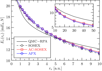
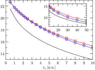
Figure 2: The Adjacent Pairs Exchange (APX) energy per electron for the uniform electron gas compared to the error of the Random Phase Approximation with respect to Quantum Monte Carlo (QMC) calculations by Ceperly and Alder³⁸, parametrized by Perdew and Zunger³⁹. The left panel shows results for the non-spin-polarized case, whereas the right panel is for the spin-polarized case. In the spin-polarized case APX slightly improves on AC-SOSEX, especially in the low density regime where the correlation energy is large compared to the kinetic energy.

$r_{s}$	$E_{\mathrm{c}}^{\mathrm{QMC}}$	$E_{\mathrm{c}}^{\mathrm{RPA}}$		$(E_{\mathrm{c}}^{\mathrm{QMC}}-E_{\mathrm{c}}^{\mathrm{RPA}})$		$E_{\mathrm{c}}^{\mathrm{SOSEX}}$	$E_{\mathrm{c}}^{\mathrm{APX}}$		$E_{\mathrm{c}}^{\mathrm{AC-SOSEX}}$
$[$a.u.$]$	[m$E_{h}\,N$]	[m$E_{h}\,N$]	$\pm$	[m$E_{h}\,N$]	$\pm$	[m$E_{h}\,N$]	[m$E_{h}\,N$]	$\pm$	[m$E_{h}\,N$]	$\pm$
1	-59.632	-78.799	0.001	19.167	0.001	19.680	19.869	0.012	19.832	0.009
2	-45.091	-61.801	0.001	16.710	0.001	17.560	17.805	0.012	17.780	0.003
3	-37.214	-52.759	$<$0.001	15.545	$<$0.001	16.090	16.347	0.012	16.342	0.003
4	-32.054	-46.806	$<$0.001	14.752	$<$0.001	14.970	15.217	0.012	15.237	0.003
5	-28.339	-42.470	$<$0.001	14.131	$<$0.001	14.070	14.297	0.012	14.343	0.003
6	-25.504	-39.117	$<$0.001	13.613	$<$0.001	13.320	13.525	0.011	13.595	0.003
7	-23.253	-36.418	$<$0.001	13.165	$<$0.001	12.670	12.863	0.011	12.955	0.003
8	-21.414	-34.182	$<$0.001	12.768	$<$0.001	12.120	12.286	0.011	12.398	0.003
9	-19.876	-32.289	$<$0.001	12.413	$<$0.001	11.620	11.777	0.011	11.906	0.003
10	-18.568	-30.658	$<$0.001	12.090	$<$0.001	11.190	11.323	0.011	11.466	0.003
12	-16.454	-27.975	$<$0.001	11.521	$<$0.001	—	10.544	0.011	10.712	0.003
15	-14.119	-24.929	$<$0.001	10.810	$<$0.001	—	9.613	0.011	9.806	0.003
20	-11.497	-21.381	$<$0.001	9.884	$<$0.001	—	8.463	0.011	8.679	0.003
30	-8.486	-17.068	$<$0.001	8.582	$<$0.001	—	6.972	0.011	7.201	0.003
40	-6.778	-14.463	$<$0.001	7.685	$<$0.001	—	6.023	0.011	6.246	0.003
50	-5.666	-12.680	$<$0.001	7.014	$<$0.001	—	5.352	0.011	5.564	0.003

Table 2: Correlation energies of the non-spin-polarized UEG as shown on the left of Figure 2, including low densities.

$r_{s}$	$E_{\mathrm{c}}^{\mathrm{QMC}}$	$E_{\mathrm{c}}^{\mathrm{RPA}}$		$(E_{\mathrm{c}}^{\mathrm{QMC}}-E_{\mathrm{c}}^{\mathrm{RPA}})$		$E_{\mathrm{c}}^{\mathrm{APX}}$		$E_{\mathrm{c}}^{\mathrm{AC-SOSEX}}$
$[$a.u.$]$	[m$E_{h}\,N$]	[m$E_{h}\,N$]	$\pm$	[m$E_{h}\,N$]	$\pm$	[m$E_{h}\,N$]	$\pm$	[m$E_{h}\,N$]	$\pm$
1	-31.701	-51.893	0.002	20.192	0.002	21.764	0.013	21.746	0.033
2	-24.090	-42.416	0.001	18.326	0.001	20.373	0.012	20.394	0.017
3	-20.048	-37.179	0.001	17.131	0.001	19.298	0.012	19.374	0.006
4	-17.415	-33.633	$<$0.001	16.218	$<$0.001	18.407	0.012	18.525	0.003
5	-15.520	-30.992	$<$0.001	15.472	$<$0.001	17.641	0.012	17.805	0.003
6	-14.071	-28.911	$<$0.001	14.840	$<$0.001	16.968	0.012	17.179	0.003
7	-12.916	-27.209	$<$0.001	14.293	$<$0.001	16.368	0.012	16.627	0.003
8	-11.969	-25.778	$<$0.001	13.809	$<$0.001	15.827	0.012	16.130	0.003
9	-11.174	-24.551	$<$0.001	13.377	$<$0.001	15.335	0.012	15.680	0.003
10	-10.495	-23.482	$<$0.001	12.987	$<$0.001	14.884	0.012	15.268	0.003
12	-9.391	-21.698	$<$0.001	12.307	$<$0.001	14.084	0.012	14.541	0.003
15	-8.160	-19.629	$<$0.001	11.469	$<$0.001	13.080	0.011	13.628	0.003
20	-6.758	-17.156	$<$0.001	10.398	$<$0.001	11.769	0.011	12.431	0.003
30	-5.112	-14.044	$<$0.001	8.932	$<$0.001	9.953	0.011	10.745	0.003
40	-4.156	-12.099	$<$0.001	7.943	$<$0.001	8.730	0.011	9.580	0.003
50	-3.521	-10.736	$<$0.001	7.215	$<$0.001	7.836	0.011	8.710	0.003

Table 3: Correlation energies of the spin-polarized UEG as shown on the right of Figure 2, including low densities.

4.2 Pair correlation functions

To assess the improvement of APX on exclusion principle violations in the RPA we evaluate the pair correlation function (PCF) $g_{\mathrm{p}}(r)$ for spin-parallel electrons in the non-spin-polarized electron gas. There are four contributions to the spin-parallel pair correlation function: the first order Hartree term, the first order exchange term, the RPA term, and the APX term. Each contribution $g^{I}(r)$ is found by a Fourier transform of the respective spin-parallel structure factor $S^{I}(q)$, in an isotropic system given by

$$g^{I}(r)=\int_{0}^{\infty}4\pi q^{2}\textrm{d}q\,\frac{\sin(qr)}{qr}\,S^{I}(q)$$ (31)

where $I$ denotes one of the four contributions enumerated above. The spin-parallel structure factor $S^{I}(q)$ is a contracted form of the reduced two-body density matrix of the form

$$S^{I}(q)=\sum_{{\mathbf{k}}_{1},{\mathbf{k}}_{2},\sigma}{\Gamma^{I}}^{({\mathbf{k}}_{1}+{\mathbf{q}})\sigma,({\mathbf{k}}_{2}-{\mathbf{q}})\sigma}_{{\mathbf{k}}_{1}\sigma,{\mathbf{k}}_{2}\sigma}$$ (32)

with ${\mathbf{q}}=(0,0,q)$. It is evaluated from the total energy diagrams contained in the contribution $I$ by taking the negative functional derivative of the total energy with respect to the Coulomb kernel $V(q)$ as outlined in Appendix A.2.

The first order Hartree contribution is constant and 1 in the uniform electron gas. The first order exchange PCF is also analytically known under the name “exchange hole”, given by $g_{\mathrm{p}}^{\mathrm{x}}(y)=-\left({3(\sin y-y\cos y)}/{y^{3}}\right)^{2}$ with $y=rk_{\mathrm{F}}$. The RPA structure factor is given by

$$S_{\mathrm{p}}^{\mathrm{RPA}}(q)=-\frac{\Omega}{N}\,\frac{1}{2}\int_{-\infty}^{\infty}\frac{\textrm{d}\nu}{2\pi}\frac{\chi_{0}(\mathrm{i}\nu,q)}{\sum_{\sigma}}\Big{\{}\Big{(}(1-\chi_{0}(\mathrm{i}\nu,q)V(q)\Big{)}^{-1}-1\Big{\}}$$ (33)

Note the division by the sum of spins to arrive at the spin-parallel structure factor. The adjacent pairs exchange structure factors is more complicated since both, $\chi_{1}(\mathrm{i}\nu,q)$ and $W(\mathrm{i}\nu,q)$ contain the Coulomb kernel $V(q)$. The resulting terms are difficult to integrate numerically such that we choose to approximate the adjacent pairs exchange terms by the terms of first order in the adjacent pairs exchange polarizability $\chi_{1}(\mathrm{i}\nu,q)$. This corresponds to restricting the APX diagrams to those containing only one exchanged interaction. The expected error is low at zero spin polarization, judging from the effect of this approximation on the total energy. The structure factor in the first order adjacent pairs exchange correction then reads

$$S_{\mathrm{p}}^{\mathrm{APX}^{(1)}}(q)=-\frac{\Omega}{N}\,\frac{1}{2}\int_{-\infty}^{\infty}\frac{\textrm{d}\nu}{2\pi}\Big{\{}(\chi^{\prime}_{1}W)(\mathrm{i}\nu,q)+\frac{\chi_{1}(\mathrm{i}\nu,q)}{\sum_{\sigma}}\Big{(}1-\chi_{0}(\mathrm{i}\nu,q)V(q)\Big{)}^{-2}\Big{\}}$$ (34)

We have transformed the momentum ${\mathbf{q}}$ to $-{\mathbf{k}}_{1}-{\mathbf{k}}_{2}-{\mathbf{q}}$ in the partial functional derivative of $\chi_{1}$ with respect to $V$ to arrive at the desired momentum $|-{\mathbf{q}}|=q$ at the removed Coulomb kernel contained in $\chi_{1}$. This gives, as a function of $q$,

$$(\chi^{\prime}_{1}W)(\mathrm{i}\nu,q)=\sum_{\sigma}\iint\limits_{F_{q}}\frac{\Omega^{2}\,\textrm{d}{\mathbf{k}}_{1}\textrm{d}{\mathbf{k}}_{2}}{(2\pi)^{6}}\left(\frac{1}{\Delta_{12}+\mathrm{i}\nu}\ \frac{1}{\Delta_{21}-\mathrm{i}\nu}\right)W(|{\mathbf{q}}+{\mathbf{k}}_{1}+{\mathbf{k}}_{2}|)$$ (35)

writing $\Delta_{ij}=\varepsilon({\mathbf{k}}_{i}+{\mathbf{q}})-\varepsilon({\mathbf{k}}_{j})$ where $i$ and $j$ are now different. Note that $\chi^{\prime}_{1}$ only contributes to the spin-parallel structure factor and no division by the number of spins is required.

The RPA structure factor and the second term of the APX⁽¹⁾ structure factor, stemming from the partial functional derivative of $W$, are integrated first over the imaginary frequency $\nu$, which is done using a Gauss–Kronrod grid with 5 subdivisions on each of the intervals $(0,1/8)\nu_{0}$, $(1/8,1/4)\nu_{0}$, $(1/4,1/2)\nu_{0}$, $(1/2,1)\nu_{0}$, $(1,2)\nu_{0}$, $(2,4)\nu_{0}$, $(4,8)\nu_{0}$, and $(8,\infty)\nu_{0}$, totaling 600 frequency samples, where $\nu_{0}=qk_{\mathrm{F}}+q^{2}/2$ is the characteristic frequency for the excitation momentum $q$. The last three intervals are transformed according to the asymptotic behavior of the integrands for large $\nu$ being proportional to $\nu^{-4}$. Evaluating the term in the APX⁽¹⁾ structure factor stemming from the partial derivative of $\chi_{1}$ is more complicated since the two momenta ${\mathbf{k}}_{1}$ and ${\mathbf{k}}_{2}$ in Eq. (35) can no longer be importance sampled independently, in contrast to Eq. (29). For each value of $q$ we now draw ${\mathbf{k}}_{1}$ and ${\mathbf{k}}_{2}$ uniformly distributed satisfying the integrand condition $|{\mathbf{k}}_{1,2}|<1<|{\mathbf{k}}_{1,2}+{\mathbf{q}}|$. Having drawn ${\mathbf{k}}_{1}$ and ${\mathbf{k}}_{2}$, the imaginary frequency $\nu$ is then subjected to importance sampling distributed with a probability density function ${\operatorname{PDF}}(u)$ proportional to the term $1/|(\Delta_{12}+\mathrm{i}\nu)(\Delta_{21}-\mathrm{i}\nu)|$ occurring in Eq. (35), where $\Delta_{ij}$ follow from $q$ and the drawn ${\mathbf{k}}_{1,2}$. The antiderivative of this PDF with respect to $\nu$ can be expressed in closed form. Note, however, that its inverse must still be found numerically. We verify above numerical procedure by computing the total APX⁽¹⁾ energy in first order of the adjacent pairs polarizability in two ways: either compute the two ended diagram containing the screened interaction $W$ and closing it with the bare interaction $V$ or vice versa. The former is computed with the method just described, the latter according to the total APX energy expression in Subsection 4.1. Both energies agree within numerical and statistical accuracy for all densities considered.

All correlated structure factor contributions are then numerically Fourier transformed on a Gauss–Kronrod grid with $32$ subdivisions on each of the intervals $(0,1/8)k_{\mathrm{F}}$, $(1/8,1/4)k_{\mathrm{F}}$, $(1/4,1/2)k_{\mathrm{F}}$, $(1/2,1)k_{\mathrm{F}}$, $(1,2)k_{\mathrm{F}}$, $(2,4)k_{\mathrm{F}}$, $(4,8)k_{\mathrm{F}}$, and $(8,\infty)k_{\mathrm{F}}$, totaling $3840$ momentum samples. The last three intervals are transformed according to the asymptotic behavior of correlated structure factor and the Fourier transform kernel $4\pi q^{2}S_{\mathrm{p}}^{I}(q)\,{\operatorname{sinc}}(qr)$ which is proportional to $q^{-3}$ for large $q$. The accuracy of the $\nu$ and $q$ integration must be considerably higher than in the total energy calculation in order to resolve Friedel oscillations.

The left panel of Figure 3 plots the resulting spin-parallel pair correlation function $g_{\mathrm{p}}(r)$ for selected densities compared to the uncorrelated exchange hole, indicated by the dotted graph. The inset enlarges the fluctuations around 1, showing the effect on the Friedel oscillations in the random phase approximation with the adjacent pairs exchange correction. To what extend APX⁽¹⁾ improves on the violations of the exclusion principle is demonstrated on the right panel of Figure 3, which contrasts the spin-parallel PCF in RPA+APX⁽¹⁾, shown in blue, to the PCF in RPA without corrections for the density $r_{\mathrm{s}}=4$. The unphysical negative on-top value of the RPA is reduced to about one half by the APX⁽¹⁾ correction in first order of the adjacent pairs exchange polarizability. The remaining error stems from RPA ring diagrams of third or higher orders which posses exchange diagrams that are not part of the APX⁽¹⁾ correction. The pair correlation functions also reveal that adjacent pairs exchange strengthens the Friedel oscillations and makes them more density dependent.

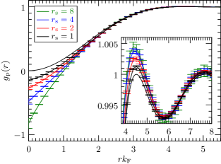
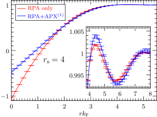
Figure 3: Left panel: pair correlation function (PCF) $g_{\mathrm{p}}(r)$ for electrons of parallel spins in the random phase approximation (RPA) including one order of the adjacent pairs exchange (APX⁽¹⁾) correction. The dotted line plots the Hartree and exchange term, known as exchange hole, marking the infinite density limit. Right panel: comparison of the PCF $g_{\mathrm{p}}(r)$ for electrons of parallel spins in the RPA with and without adjacent pairs exchange correction. Exchange considerably improves on the unphysical negative part close to the coalescence point $r=0$. Its effect on the Friedel oscillations is shown in the inset. The error bars in both plots denote the 95% confidence interval.

5 Summary

The particle/hole bubbles of the random phase approximation contain contributions where two or more states propagate at the same instance in time. Such Pauli exclusion principle violating (EPV) contributions would be canceled in the full many-body perturbation expansion by exchange terms. Their absence lets the random phase approximation overestimate the absolute values of the correlation energy. Here, we propose the adjacent pairs exchange (APX) correction as the largest set of diagrams, such that

1. each diagram is an exchange diagram of RPA,

2. introducing no further EPV contributions, and

3. the resulting diagrams can be computed in $\mathcal{O}(N^{4})$ in real-space.

The last point relates to $\mathcal{O}(N^{4})$ being the next higher class of computational complexity following RPA’s $\mathcal{O}(N^{3})$ complexity. The APX is constructed by exchanging states of adjacent pair bubbles in RPA diagrams, where the Coulomb interaction occurs at the end of both bubbles

$${\mathbf{X}}_{0}{\mathbf{V}}{\mathbf{X}}_{0}=\raisebox{2.15277pt}{\includegraphics{Chi0VChi0pm}}\ \mapsto\ \raisebox{2.15277pt}{\includegraphics{Chi1Small}}={\mathbf{X}}_{1}$$ (36)

In terms of Feynman diagrams, the APX is given by

$$E_{\mathrm{c}}^{\mathrm{APX}}=\raisebox{2.15277pt}{\includegraphics{Ring1Apx}}\ +\ \raisebox{2.15277pt}{\includegraphics{Ring2Apx}}\ +\ \raisebox{2.15277pt}{\includegraphics{Ring3Apx}}\ +\ \ldots$$ (37)

Appendix A lists the detailed expressions for the correlation energy, as well as for the correlation contribution to expectation values. Inherited from RPA, APX contains up to an infinite number of exchange processes, unlike second order screened exchange variants, such as SOSEX and AC-SOSEX. The difference is small though, since APX differs from SOSEX only from fourth order onward. In spin-polarized systems the difference is larger since ${\mathbf{X}}_{1}$ and the replaced pair bubbles are more similar in magnitude, however, having opposite signs. We apply the proposed method to the uniform electron gas, numerically integrating the occurring propagators to provide basis-set converged benchmark numbers in the thermodynamic limit. It remains to be studied, how APX performs with respect to other comparable screened exchange corrections in various chemical environments.

Appendix A Computing the adjacent pairs exchange correction

This section derives all expressions of this work used to compute RPA+APX total energies and expectation values. We use imaginary time dependent many-body perturbation theory to construct the building blocks of the respective terms, which are in turn transform to imaginary frequencies in order to concatenate them to the ring-formed diagrams of the random phase approximation and of the adjacent pairs exchange correction. The final imaginary frequency integration can be done numerically on a relatively small grid whose size is independent of the system size. ^{40, 10} It is fit to best approximate the analytically known imaginary frequency integral in MP2 $\int_{0}^{\infty}\textrm{d}\nu/2\pi\times 2/({\Delta^{2}}^{a}_{i}+\nu^{2})=1/2\Delta^{a}_{i}$ by a numerical quadrature, writing $\Delta^{a}_{i}=\varepsilon_{a}-\varepsilon_{i}$. For efficiency, the optimization is restricted to states of the MP2 terms where $a=b$ and $i=j$. The quadrature weights and points are thus found by

$$(w_{n},\nu_{n})=\underset{(w_{n},\,\nu_{n})}{\mathrm{argmin}}\left\|\frac{1}{2\Delta^{a}_{i}}-\sum_{n}w_{n}\frac{2}{{\Delta^{2}}^{a}_{i}+\nu^{2}_{n}}\right\|_{2}^{2}$$ (38)

which is a separable non-linear least squares problem and can be fit by the variable projection algorithm as implemented in varpro.⁴¹ How to setup the imaginary time grid and the Fourier transform between the grids is described in Ref. 10. Appendix B briefly outlines the diagrammatic techniques of imaginary time dependent MBPT employed here.

The unperturbed propagators for particles, holes, and Coulomb interactions are given by

$${G_{0}}^{{\mathbf{x}}_{2}}_{{\mathbf{x}}_{1}}(\mathrm{i}\tau_{12}) =+\sum_{a}\psi_{a}({\mathbf{x}}_{2})\,{\mathrm{e}}^{-\varepsilon^{\prime}_{a}\tau_{12}}\,{\psi^{\ast}}^{a}({\mathbf{x}}_{1}) \,:\tau_{12}>0$$ (39)

$${G_{0}}^{{\mathbf{x}}_{2}}_{{\mathbf{x}}_{1}}(\mathrm{i}\tau_{12}) =-\sum_{i}{\psi^{\ast}}^{i}({\mathbf{x}}_{1})\,{\mathrm{e}}^{-\varepsilon^{\prime}_{i}\tau_{12}}\,\psi_{i}({\mathbf{x}}_{2}) \,:\tau_{12}\leq 0$$ (40)

$$V^{{\mathbf{x}}_{2}}_{{\mathbf{x}}_{1}} =(-1)/|{\mathbf{r}}_{1}-{\mathbf{r}}_{2}|$$ (41)

respectively, where $\tau_{12}=\tau_{2}-\tau_{1}$ is the imaginary time difference between the starting point ${\mathbf{x}}_{1}$ and the endpoint ${\mathbf{x}}_{2}$ of the propagator. The Coulomb interaction is assumed to act instantaneously.

From them, we construct the matrizes of the independent particle polarizability

$${X_{0}}^{{\mathbf{x}}_{2}}_{{\mathbf{x}}_{1}}(\mathrm{i}\tau_{12})=\raisebox{2.15277pt}{\includegraphics{Chi0}}=(-1)^{1}\,{G_{0}}^{{\mathbf{x}}_{2}}_{{\mathbf{x}}_{1}}(\mathrm{i}\tau_{12})\,{G_{0}}^{{\mathbf{x}}_{1}}_{{\mathbf{x}}_{2}}(\mathrm{i}\tau_{21})$$ (42)

and the adjacent pairs exchange polarizability

$${X_{1}}^{{\mathbf{x}}_{2}}_{{\mathbf{x}}_{1}}(\mathrm{i}\tau_{13},\mathrm{i}\tau_{23})=\raisebox{2.15277pt}{\includegraphics{Chi1}}=\iint\textrm{d}{\mathbf{x}}_{3}\,\textrm{d}{\mathbf{x}}_{4}\\ (-1)^{1}\,V^{{\mathbf{x}}_{3}}_{{\mathbf{x}}_{4}}\,{G_{0}}^{{\mathbf{x}}_{3}}_{{\mathbf{x}}_{1}}(\mathrm{i}\tau_{13})\,{G_{0}}^{{\mathbf{x}}_{2}}_{{\mathbf{x}}_{3}}(\mathrm{i}\tau_{32})\,{G_{0}}^{{\mathbf{x}}_{4}}_{{\mathbf{x}}_{2}}(\mathrm{i}\tau_{23})\,{G_{0}}^{{\mathbf{x}}_{1}}_{{\mathbf{x}}_{4}}(\mathrm{i}\tau_{31})$$ (43)

for $\tau_{13},\tau_{23}>0$. For all other time orderings it is ${\mathbf{0}}$ according to the chosen time order of the exchanged adjacent pairs. Note that $\tau_{3}=\tau_{4}$. Fourier-transforming with respect to the imaginary time between 1 and 2 yields

$${\mathbf{X}}_{0}(\mathrm{i}\nu)= \int_{-\infty}^{\infty}\textrm{d}\tau_{12}\,{\mathrm{e}}^{-\mathrm{i}\nu\tau_{12}}\,{\mathbf{X}}_{0}(\mathrm{i}\tau_{12})$$ (44)

$${\mathbf{X}}_{1}(\mathrm{i}\nu)= \iint_{0}^{\infty}\textrm{d}\tau_{13}\,\textrm{d}\tau_{23}\,{\mathrm{e}}^{-\mathrm{i}\nu\tau_{12}}\,{\mathbf{X}}_{1}(\mathrm{i}\tau_{13},\mathrm{i}\tau_{23})$$ (45)

where $\tau_{12}=\tau_{13}-\tau_{23}$ in Eq. (45). See Ref. 10 for numerical details on the choice of the imaginary time and frequency grid, as well as on the Fourier transform on the non-equidistant grid. Defining the matrix operations

$$\left({\mathbf{A}}{\mathbf{B}}\right)^{{\mathbf{x}}_{3}}_{{\mathbf{x}}_{1}} =\int\textrm{d}{\mathbf{x}}_{2}\,A^{{\mathbf{x}}_{2}}_{{\mathbf{x}}_{1}}B^{{\mathbf{x}}_{3}}_{{\mathbf{x}}_{2}}$$ (46)

$${\operatorname{Tr}}\left\{{\mathbf{A}}\right\} =\int\textrm{d}{\mathbf{x}}\,A^{{\mathbf{x}}}_{{\mathbf{x}}}$$ (47)

$$\left({\mathbf{A}}^{T}\right)^{{\mathbf{x}}_{2}}_{{\mathbf{x}}_{1}} =A^{{\mathbf{x}}_{1}}_{{\mathbf{x}}_{2}}$$ (48)

we can now assemble the quantities of interest from the imaginary frequency dependent diagrammatic building blocks ${\mathbf{X}}_{0}$ and ${\mathbf{X}}_{1}$, and the instantaneous, thus frequency independent, bare Coulomb interaction ${\mathbf{V}}$. We start by defining the RPA-screened interaction

$${\mathbf{W}}(\mathrm{i}\nu)=\ \raisebox{2.15277pt}{\includegraphics{W}}\ =\ \raisebox{2.15277pt}{\includegraphics{V}}\ +\ \raisebox{2.15277pt}{\includegraphics{VChi0V}}\ +\ \ldots\\ ={\mathbf{V}}+{\mathbf{V}}{\mathbf{X}}_{0}{\mathbf{V}}+\ldots={\mathbf{V}}\big{(}{\mathbf{1}}-{\mathbf{X}}_{0}(\mathrm{i}\nu){\mathbf{V}}\big{)}^{-1}$$ (49)

which assumes no change of symmetries when inserting ${\mathbf{X}}_{0}$. Otherwise, the symmetry factor must be considered order by order, as done for the RPA correlation energy.

A.1 Correlation Energy

The correlation energy in the random phase approximation is the sum of all ring diagrams which are concatenated from independent particle polarizability diagrams ${\mathbf{X}}_{0}$ connected by bare electron interactions ${\mathbf{V}}$. At least two polarizability diagrams are required, so the lowest order is $2$. The diagram of order $n$ exhibits an $n$ fold rotational symmetry, such that the respective requires a factor of $1/n$ to prevent multiple counting. Details on the evaluation of Feynman diagrams are given in Appendix B.2. The RPA correlation energy thus reads

$$E_{\mathrm{c}}^{\mathrm{RPA}}=\raisebox{2.15277pt}{\includegraphics{Ring2}}+\ \raisebox{2.15277pt}{\includegraphics{Ring3}}+\ \ldots=-\frac{1}{2}\left[\frac{1}{2}\,{\mathbf{X}}_{0}{\mathbf{V}}{\mathbf{X}}_{0}{\mathbf{V}}+\frac{1}{3}\,{\mathbf{X}}_{0}{\mathbf{V}}{\mathbf{X}}_{0}{\mathbf{V}}{\mathbf{X}}_{0}{\mathbf{V}}+\ldots\right]\\ =\frac{1}{2}\int_{-\infty}^{\infty}\frac{\textrm{d}\nu}{2\pi}\,{\operatorname{Tr}}\left\{\log\big{(}{\mathbf{1}}-{\mathbf{X}}_{0}(\mathrm{i}\nu){\mathbf{V}}\big{)}+{\mathbf{X}}_{0}(\mathrm{i}\nu){\mathbf{V}}\right\}$$ (50)

where we omit the trace and the imaginary frequency arguments in the explicit expansion, given in the second line. Analogously, the adjacent pairs exchange correction is the sum of all ring diagrams which are concatenated from adjacent pairs exchange polarizability diagrams ${\mathbf{X}}_{1}$ connected by screened electron interactions ${\mathbf{W}}$. The lowest number of occurrences of ${\mathbf{X}}_{1}$ is one since ${\mathbf{X}}_{1}$ already contains one bare interaction ${\mathbf{V}}$. The APX diagrams also exhibit rotational symmetry and the APX correction to the correlation energy is thus given by

$$E_{\mathrm{c}}^{\mathrm{APX}}=\raisebox{2.15277pt}{\includegraphics{Ring1Apx}}\ +\ \raisebox{2.15277pt}{\includegraphics{Ring2Apx}}\ +\ \raisebox{2.15277pt}{\includegraphics{Ring3Apx}}\ +\ \ldots\\ =\frac{1}{2}\int_{-\infty}^{\infty}\frac{\textrm{d}\nu}{2\pi}\,{\operatorname{Tr}}\left\{\log\big{(}{\mathbf{1}}-{\mathbf{X}}_{1}(\mathrm{i}\nu){\mathbf{W}}(\mathrm{i}\nu)\big{)}\right\}$$ (51)

A.2 Expectation values

Given the expression for the correlation energies we can consistently evaluate correlation corrections to expectation values of operators from the Güttinger or Hellman–Feynman theorem, as detailed in Appendix B.3. Here we only give an expression for local, symmetric two-body operators.

Given a symmetric two-body operator, local in real space,

$$\hat{B}=\raisebox{2.15277pt}{\includegraphics{B}}=\sum_{pqrs}B^{pq}_{sr}\hat{c}_{p}^{\dagger}\hat{c}_{q}^{\dagger}\hat{c}_{r}\hat{c}_{s}$$ (52)

with

$$B^{pq}_{sr}=\iint\limits_{\textrm{d}{\mathbf{x}}_{1}\,\textrm{d}{\mathbf{x}}_{2}}{\psi^{\ast}}^{p}({\mathbf{x}}_{1})\,{\psi^{\ast}}^{q}({\mathbf{x}}_{2})\,B^{{\mathbf{x}}_{2}}_{{\mathbf{x}}_{1}}\psi_{r}({\mathbf{x}}_{2})\,\psi_{s}({\mathbf{x}}_{1})$$ (53)

we construct the adjacent pairs polarizability, where the bare electron interaction is replaced by the operator $\hat{B}$

$${X_{1}^{B}}^{{\mathbf{x}}_{2}}_{{\mathbf{x}}_{1}}(\mathrm{i}\tau_{13},\mathrm{i}\tau_{23})=\raisebox{2.15277pt}{\includegraphics{Chi1B}}=\iint\textrm{d}{\mathbf{x}}_{3}\,\textrm{d}{\mathbf{x}}_{4}\\ (-1)^{1}\,B^{{\mathbf{x}}_{3}}_{{\mathbf{x}}_{4}}\,{G_{0}}^{{\mathbf{x}}_{3}}_{{\mathbf{x}}_{1}}(\mathrm{i}\tau_{13})\,{G_{0}}^{{\mathbf{x}}_{2}}_{{\mathbf{x}}_{3}}(\mathrm{i}\tau_{32})\,{G_{0}}^{{\mathbf{x}}_{4}}_{{\mathbf{x}}_{2}}(\mathrm{i}\tau_{23})\,{G_{0}}^{{\mathbf{x}}_{1}}_{{\mathbf{x}}_{4}}(\mathrm{i}\tau_{31})$$ (54)

for $\tau_{13},\tau_{23}>0$ and 0 otherwise. It Fourier transform with respect to the imaginary time difference between 1 and 2 reads

$${\mathbf{X}}_{1}^{B}(\mathrm{i}\nu)=\iint_{0}^{\infty}\textrm{d}\tau_{13}\,\textrm{d}\tau_{23}\,{\mathrm{e}}^{-\mathrm{i}\nu\tau_{12}}\,{\mathbf{X}}_{1}^{B}(\mathrm{i}\tau_{13},\mathrm{i}\tau_{23})$$ (55)

where $\tau_{12}=\tau_{13}-\tau_{23}$. We also construct the RPA-screened interaction where one of the bare interactions is replaced by the operator $\hat{B}$

$${{\mathbf{W}}^{B}}(\mathrm{i}\nu)={\mathbf{B}}+2{\mathbf{B}}{\mathbf{X}}_{0}{\mathbf{V}}+3{\mathbf{B}}{\mathbf{X}}_{0}{\mathbf{V}}{\mathbf{X}}_{0}{\mathbf{V}}+\ldots={\mathbf{B}}\big{(}{\mathbf{1}}-{\mathbf{X}}_{0}(\mathrm{i}\nu){\mathbf{V}}\big{)}^{-2}$$ (56)

which assumes no change of symmetries when inserting ${\mathbf{X}}_{0}$.

Finally, we write the terms of the correlation contribution to $\langle\hat{B}\rangle$. They are constructed from the diagrams of the correlation energy by summing all possibilities of replacing one of the Coulomb interactions ${\mathbf{V}}$ by the operator $\hat{B}$. For the RPA and APX this gives, respectively

$$\langle\hat{B}\rangle^{\mathrm{RPA}}=\raisebox{2.15277pt}{\includegraphics{Ring2B}}\ +\ \raisebox{2.15277pt}{\includegraphics{Ring3B}}\ +\ \ldots=-\frac{1}{2}\Big{[}{\mathbf{B}}{\mathbf{X}}_{0}{\mathbf{V}}{\mathbf{X}}_{0}+{\mathbf{B}}{\mathbf{X}}_{0}{\mathbf{V}}{\mathbf{X}}_{0}{\mathbf{V}}{\mathbf{X}}_{0}+\ldots\Big{]}\\ =-\frac{1}{2}\int_{-\infty}^{\infty}\frac{\textrm{d}\nu}{2\pi}\,{\operatorname{Tr}}\Big{\{}{{\mathbf{B}}}{\mathbf{X}}_{0}(\mathrm{i}\nu){\mathbf{W}}(\mathrm{i}\nu){\mathbf{X}}_{0}(\mathrm{i}\nu)\Big{\}}$$ (57)

$$\langle\hat{B}\rangle^{\mathrm{APX}}=\raisebox{2.15277pt}{\includegraphics{Apx2B}}\ +\ \raisebox{2.15277pt}{\includegraphics{Apx3B}}\ +\ \ldots\ +\ \raisebox{2.15277pt}{\includegraphics{Apx3UpsilonB}}\ +\ \raisebox{2.15277pt}{\includegraphics{Apx4B}}\ +\ \ldots\\ =-\frac{1}{2}\Big{[}{\mathbf{X}}^{B}_{1}{\mathbf{W}}+{\mathbf{X}}^{B}_{1}{\mathbf{W}}{\mathbf{X}}_{1}{\mathbf{W}}+\ldots+{\mathbf{X}}_{1}{\mathbf{W}}^{B}+{\mathbf{X}}_{1}{\mathbf{W}}^{B}{\mathbf{X}}_{1}{\mathbf{W}}+\ldots\Big{]}\\ =-\frac{1}{2}\int_{-\infty}^{\infty}\frac{\textrm{d}\nu}{2\pi}\,{\operatorname{Tr}}\Big{\{}\big{(}{\mathbf{X}}^{B}_{1}(\mathrm{i}\nu){\mathbf{W}}(\mathrm{i}\nu)+{\mathbf{X}}_{1}(\mathrm{i}\nu){\mathbf{W}}^{B}(\mathrm{i}\nu)\big{)}\times\big{(}{\mathbf{1}}-{\mathbf{X}}_{1}(\mathrm{i}\nu){\mathbf{W}}(\mathrm{i}\nu)\big{)}^{-1}\Big{\}}$$ (58)

where the rotational symmetry is again broken while the time reversal symmetry remains. Note that the pair correlation function computed according to the above equations yields the potential energy rather than the correlation energy when integrated with the Coulomb kernel.

Appendix B Evaluation of diagrams

This appendix summarized the translation between diagrams and algebraic expressions of many-body perturbation theory used in in this work. More details can be found e.g. in Refs. 42, 25, 29.

B.1 Goldstone diagrams

Goldstone diagrams depict the non-relativistic instantaneous Coulomb interactions by horizontal wiggly lines with time moving forward from bottom to top. The time order of the interactions is fixed by the order in the diagram. The occupation of electronic states is given relative to the ground state of the Hartree–Fock or DFT reference. Spin-orbital states which are unoccupied in the reference are called particle states, denoted by the letters $a,b,c,\ldots$ spin-orbital states which are occupied in the reference are called hole states, denoted by the letters $i,j,k,\ldots$ Particle and hole states are depicted by arrows pointing upwards and downwards, respectively.

Goldstone diagrams are evaluated by contracting the electron repulsion integrals tensor

$$V^{pq}_{sr}=\\ \iint\limits_{\textrm{d}{\mathbf{x}}_{1}\,\textrm{d}{\mathbf{x}}_{2}}{\psi^{\ast}}^{p}({\mathbf{x}}_{1})\,{\psi^{\ast}}^{q}({\mathbf{x}}_{2})\,\frac{1}{|{\mathbf{r}}_{2}-{\mathbf{r}}_{1}|}\psi_{r}({\mathbf{x}}_{2})\,\psi_{s}({\mathbf{x}}_{1})$$ (59)

over the states of connected interactions. Incomming indices are written downstairs, outgoing indices upstairs. Indices from connections on the left vertex are standing left. As an example the second order term of the RPA evaluates to

$$\raisebox{2.15277pt}{\includegraphics{Ring2StatesLabeled.pdf}}=\frac{1}{2}\,(-1)^{(2+2)}\,\frac{V^{ab}_{ij}\,V^{ij}_{ab}}{(-\Delta^{ab}_{ij})}$$ (60)

with $\Delta^{ab}_{ij}=\varepsilon_{a}+\varepsilon_{b}-\varepsilon_{i}-\varepsilon_{j}$ and implying a sum over all states occurring only on the right hand side. Each interval between two successive Coulomb interactions gives rise to a negative energy denominator, subtracting all particle energies from all hole energies of states propagating in the respective interval.

Additionally, the symmetry factor and the fermion sign must be determined. One Goldstone diagram represents all $2^{n}$ Wick contractions generated by interchanging left and right indices on each of the $n$ Coulomb interactions. If, however, the entire diagram exhibits a left/right mirror symmetry only half of the Wick contractions are distinct. In this case the diagram must be divided by two upon evaluation. The fermion sign of a Goldstone diagram is $(-1)^{(l+h)}$ where $l$ denotes the number of closed fermion loops and $h$ denotes the number of hole connection, both of which are 2 in the above example.

B.2 Feynman diagrams

Feynman diagrams depict the Coulomb interaction by wiggly lines which are not necessarily horizontal and there is no notion of a forward time direction. A single Feynman diagram represents all possible time orders of the interactions involved, which are instantaneous. In $n$th order one Feynman diagram represents in general $n!$ Goldstone diagrams corresponding to the possible permutations of the occurring interactions.

Feynman diagrams can be evaluated by integrating the product of all fermion and boson propagators over position and time of each vertex. We choose to apply the Wick rotation $t=\mathrm{i}\tau$, $\varepsilon^{\prime}_{p}=\varepsilon_{p}-\varepsilon_{\mathrm{F}}$ to move the frequency integration contour away from the poles of the fermion propagator $G_{0}$. The second order term of the RPA then evaluates to

$$(-1)\raisebox{2.15277pt}{\includegraphics{Ring2Labeled.pdf}}=\frac{1}{2\cdot 2}(-1)^{2}\iiiint\textrm{d}1\,\textrm{d}2\,\textrm{d}3\,\textrm{d}4\,\delta(\tau_{1})\\ V(1,4)\,V(2,3)\,G_{0}(1,2)\,G_{0}(2,1)\,G_{0}(3,4)\,G_{0}(4,3)$$ (61)

with the shorthand notation $\int\textrm{d}n=\sum_{\sigma_{n}}\int\textrm{d}{\mathbf{r}}_{n}\int_{-\infty}^{\infty}\textrm{d}\tau_{n}$. Note that the single Dirac delta $\delta(\tau_{1})$ is only required in the time domain. In the non-relativistic case the fermion propagator $G_{0}$ and the boson propagator $V$ are given by

$$G_{0}(n,m)= +\sum_{a}\psi_{a}({\mathbf{x}}_{n})\,{\psi^{\ast}}^{a}({\mathbf{x}}_{m})\,{\mathrm{e}}^{-\varepsilon^{\prime}_{a}\tau} :\tau>0\quad$$ (62)

$$G_{0}(n,m)= -\sum_{i}\psi_{i}({\mathbf{x}}_{n})\,{\psi^{\ast}}^{i}({\mathbf{x}}_{m})\,{\mathrm{e}}^{-\varepsilon^{\prime}_{i}\tau} :\tau\leq 0\quad$$ (63)

$$V(n,m)= -\delta(\tau)/|{\mathbf{r}}_{m}-{\mathbf{r}}_{n}|$$ (64)

with $\tau=\tau_{n}-\tau_{m}$.

Additionally, the symmetry factor and the fermion sign must be determined. In the case of above diagram there are two vertex permutations forming the group of all symmetry operations leaving the diagram invariant:

$$M=1234\mapsto 4321,\quad R_{2}=1234\mapsto 3412$$ (65)

corresponding to the left/right mirror operation and the $180^{\circ}$ rotation, respectively. Both operations have order 2, such that only one fourth of all possible permutations of the vertices yield distinct contractions. Thus, the diagram must be divided by 4 upon evaluation. The fermion sign for each hole propagator and for each closed fermion propagator loop is $(-1)$. In imaginary time each Coulomb interaction as well as a closed diagram also come with a factor of $(-1)$. The sign of the propagators are taken into account by Eq. (63) and (64) such that only the number of loops and whether the diagram is closed or not need to be considered.

B.3 Expectation values

The expectation value of an operator $\hat{A}$ is related to the ground state energy with the modified Hamiltonian $\hat{H}(\lambda\hat{A})=\hat{H}+\lambda\hat{A}$ by the Güttinger⁴³ or Hellman–Feynman theorem

$$\langle\hat{A}\rangle=\frac{\langle\Psi|\hat{A}|\Psi\rangle}{\langle\Psi|\Psi\rangle}=\left.\frac{\textrm{d}}{\textrm{d}\lambda}E(\lambda\hat{A})\,\right|_{\lambda=0}$$ (66)

In an approximate theory the right hand side of Eq. (66) approaches the expectation value of $\hat{A}$ as the modified ground state wave function $|\Psi(\lambda\hat{A})\rangle$ becomes an eigenstate of $\hat{H}(\lambda\hat{A})$ to the eigenvalue $E(\lambda\hat{A})$ with increasing quality of approximation, irrespective of whether it is a variational approximation or not. In perturbation theory the right hand side of Eq. (66) is evaluated by a projection ansatz

$$\left.\frac{\textrm{d}}{\textrm{d}\lambda}E(\lambda\hat{A})\,\right|_{\lambda=0}=\left.\frac{\textrm{d}}{\textrm{d}\lambda}\big{\langle}\Phi|\hat{H}_{0}+\hat{H}_{1}+\lambda\hat{A}|\Psi(\lambda\hat{A})\big{\rangle}^{\prime}\,\right|_{\lambda=0}$$ (67)

where $|\Psi(\lambda\hat{A})\rangle$ is the ground state wave function $|\Phi\rangle$ of the reference Hamiltonian $\hat{H}_{0}$ subjected to the perturbation $\hat{H}_{1}+\lambda\hat{A}$ and where $\langle\cdot|\cdot|\cdot\rangle^{\prime}$ denotes contractions over connected terms only.

We compute Eq. (67) for two-body operators $\hat{B}$ by treating $\lambda\hat{B}$ as an additional perturbation to $\hat{H}_{1}$ while for one-body operators $\hat{A}$ we add $\lambda\hat{A}$ to $\hat{H}_{0}$, expanding the occurring exponentials in first order. This treatment leads to consistent energy expectation values in the sense that

$$\langle\hat{H}\rangle=\langle\hat{H}_{0}\rangle+\langle\hat{H}_{1}\rangle$$ (68)

holds exactly at any level of approximation, rather than just asymptotically in the fully approximating limit. From a given ground state diagram a two-body operator $\langle\hat{B}\rangle$ is thus evaluated by replacing each occurrence of a wiggly line $\hat{H}_{1}$ by the operator $\hat{B}$, while a one-body operator $\hat{A}$ is evaluated by insertion between successive occurrences of two wiggly lines $\hat{H}_{1}$.

References

- Harl et al. 2010 Harl, J.; Schimka, L.; Kresse, G. Assessing the quality of the random phase approximation for lattice constants and atomization energies of solids. Phys. Rev. B 2010, 81, 115126
- Macke 1950 Macke, W. Über die Wechselwirkungen im Fermi-Gas, Polarisationserscheinungen, Correlationsenergie, Elektronenkondensation. Z. Naturforsch. 1950, 5a, 192–208
- Pines and Bohm 1952 Pines, D.; Bohm, D. A Collective Description of Electron Interactions: II. Collective vs Individual Particle Aspects of the Interactions. Phys. Rev. 1952, 85, 338–353
- Dreuw and Head-Gordon 2005 Dreuw, A.; Head-Gordon, M. Single-Reference ab Initio Methods for the Calculation of Excited States of Large Molecules. Chem. Rev. 2005, 105, 4009–4037
- Furche 2001 Furche, F. Molecular tests of the random phase approximation to the exchange-correlation energy functional. Phys. Rev. B 2001, 64, 195120
- Grüneis et al. 2009 Grüneis, A.; Marsman, M.; Harl, J.; Schimka, L.; Kresse, G. Making the random phase approximation to electronic correlation accurate. J. Chem. Phys. 2009, 131, 154115
- Monkhorst and Oddershede 1973 Monkhorst, H. J.; Oddershede, J. Random-Phase-Approximation Correlation Energy in Metallic Hydrogen Using Hartree-Fock Bloch Functions. Phys. Rev. Lett. 1973, 30, 797–800
- Freeman 1977 Freeman, D. Coupled-cluster expansion applied to the electron gas: Inclusion of ring and exchange effects. Phys. Rev. B 1977, 15, 5512–5521
- Rojas et al. 1995 Rojas, H.; Godby, R.; Needs, R. Space-Time Method for Ab Initio Calculations of Self-Energies and Dielectric Response Functions of Solids. Phys. Rev. Lett. 1995, 74, 1827–1830
- Kaltak et al. 2014 Kaltak, M.; Kresse, G.; Klimeš, J. Low Scaling Algorithms for the Random Phase Approximation: Imaginary Time and Laplace Transformations. J. Chem. Theory Comput. 2014, 10, 2498–2507
- Chen et al. 2018 Chen, G. P.; Agee, M. M.; Furche, F. Performance and Scope of Perturbative Corrections to Random-Phase Approximation Energies. J. Chem. Theory Comput. 2018, 14, 5701–5714
- Furche 2008 Furche, F. Developing the random phase approximation into a practical post-Kohn–Sham correlation model. J. Chem. Phys. 2008, 129, 114105
- Harl and Kresse 2009 Harl, J.; Kresse, G. Accurate Bulk Properties from Approximate Many-Body Techniques. Phys. Rev. Lett. 2009, 103, 056401
- Schimka et al. 2010 Schimka, L.; Harl, J.; Stroppa, A.; Grüneis, A.; Marsman, M.; Mittendorfer, F.; Kresse, G. Accurate surface and adsorption energies from many-body perturbation theory. Nat. Mat. 2010, 9, 741–744
- Lebègue et al. 2010 Lebègue, S.; Harl, J.; Gould, T.; Ángyán, J. G.; Kresse, G.; Dobson, J. F. Cohesive properties and asymptotics of the dispersion interaction in graphite by the random phase approximation. Phys. Rev. Lett. 2010, 105, 196401
- Paier et al. 2012 Paier, J.; Ren, X.; Rinke, P.; Scuseria, G. E.; Grüneis, A.; Kresse, G.; Scheffler, M. Assessment of correlation energies based on the random-phase approximation. New J. Phys. 2012, 14, 043002
- Klimeš et al. 2015 Klimeš, J.; Kaltak, M.; Maggio, E.; Kresse, G. Singles correlation energy contributions in solids. J. Chem. Phys. 2015, 143, 102816
- Garrido Torres et al. 2017 Garrido Torres, J. A.; Ramberger, B.; Früchtl, H. A.; Schaub, R.; Kresse, G. Adsorption energies of benzene on close packed transition metal surfaces using the random phase approximation. Phys. Rev. Materials 2017, 1, 060803
- Wick 1950 Wick, G. C. The Evaluation of the Collision Matrix. Phys. Rev. 1950, 80, 268–272
- Goldstone 1957 Goldstone, J. Derivation of the Brueckner Many-Body Theory. Proc. Royal Soc. A 1957, 239, 267–279
- Holzer et al. 2018 Holzer, C.; Gui, X.; Harding, M. E.; Kresse, G.; Helgaker, T.; Klopper, W. Bethe–Salpeter correlation energies of atoms and molecules. J. Chem. Phys. 2018, 149, 144106
- Ángyán et al. 2011 Ángyán, J. G.; Liu, R.-F.; Toulouse, J.; Jansen, G. Correlation Energy Expressions from the Adiabatic-Connection Fluctuation–Dissipation Theorem Approach. J. Chem. Theory Comput. 2011, 7, 3116–3130
- Bates and Furche 2013 Bates, J. E.; Furche, F. Communication: Random phase approximation renormalized many-body perturbation theory. J. Chem. Phys. 2013, 139, 171103
- Nooijen and Snijders 1993 Nooijen, M.; Snijders, J. G. Diagrammatic analysis and application of the coupled cluster response approach to ground-state expectation values. Int. J. Quantum Chem. 1993, 47, 3–47
- Thouless 2014 Thouless, D. J. The quantum mechanics of many-body systems, second dover edition ed.; Dover Publications, Inc: Mineola, New York, 2014
- Shavitt and Bartlett 2009 Shavitt, I.; Bartlett, R. J. Many-body methods in chemistry and physics: MBPT and coupled-cluster theory; Cambridge University Press, 2009
- Scuseria et al. 2008 Scuseria, G. E.; Henderson, T. M.; Sorensen, D. C. The ground state correlation energy of the random phase approximation from a ring coupled cluster doubles approach. J. Chem. Phys. 2008, 129, 231101
- Čížek 1969 Čížek, J. In Advances in Chemical Physics; LeFebvre, R., Moser, C., Eds.; John Wiley & Sons, Inc., 1969; pp 35–89
- Hummel 2015 Hummel, F. A. Density functional theory applied to liquid metals and the adjacent pairs exchange correction to the random phase approximation. Ph.D. thesis, University of Vienna, Vienna, 2015
- Szabo and Ostlund 1977 Szabo, A.; Ostlund, N. S. Interaction energies between closed-shell systems: The correlation energy in the random phase approximation. Int. J. Quantum Chem. 1977, 12, 389–395
- Szabo and Ostlund 1977 Szabo, A.; Ostlund, N. S. The correlation energy in the random phase approximation: Intermolecular forces between closed-shell systems. J. Chem. Phys. 1977, 67, 4351–4360
- Maggio and Kresse 2016 Maggio, E.; Kresse, G. Correlation energy for the homogeneous electron gas: Exact Bethe-Salpeter solution and an approximate evaluation. Phys. Rev. B 2016, 93, 235113
- Coester and Kümmel 1960 Coester, F.; Kümmel, H. Short-range correlations in nuclear wave functions. Nucl. Phys. 1960, 17, 477–485
- Gell-Mann and Brueckner 1957 Gell-Mann, M.; Brueckner, K. A. Correlation Energy of an Electron Gas at High Density. Phys. Rev. 1957, 106, 364–368
- Scuseria et al. 2013 Scuseria, G. E.; Ren, X.; Rinke, P.; Scheffler, M. Renormalized second-order perturbation theory for the electron correlation energy: Concept, implementation, and benchmarks. Phys. Rev. B 2013, 88, 035120
- Sander et al. 2015 Sander, T.; Maggio, E.; Kresse, G. Beyond the Tamm–Dancoff approximation for extended systems using exact diagonalization. Phys. Rev. B 2015, 92, 045209
- Ziesche 2010 Ziesche, P. The high-density electron gas: How momentum distribution and static structure factor are mutually related through the off-shell self-energy. Ann. Phys. (Berl.) 2010, 522, 739–765
- Ceperley and Alder 1980 Ceperley, D. M.; Alder, B. J. Ground State of the Electron Gas by a Stochastic Method. Phys. Rev. Lett. 1980, 45, 566–569
- Perdew and Zunger 1981 Perdew, J. P.; Zunger, A. Self-interaction correction to density-functional approximations for many-electron systems. Phys. Rev. B 1981, 23, 5048–5079
- Almlöf 1991 Almlöf, J. Elimination of energy denominators in Møller—Plesset perturbation theory by a Laplace transform approach. Chem. Phys. Lett. 1991, 181, 319–320
- Golub and Pereyra 1973 Golub, G. H.; Pereyra, V. The Differentiation of Pseudo-Inverses and Nonlinear Least Squares Problems Whose Variables Separate. SIAM J. Numer. Anal. 1973, 10, 413–432
- Szabo and Ostlund 1996 Szabo, A.; Ostlund, N. S. Modern quantum chemistry: introduction to advanced electronic structure theory; Dover Publications, 1996
- Güttinger 1932 Güttinger, P. Das Verhalten von Atomen im magnetischen Drehfeld. Z. Physik 1932, 73, 169–184