Computing the topological susceptibility from fixed topology QCD simulations

Abstract

The topological susceptibility is an important quantity in QCD, which can be computed using lattice methods. However, at a fine lattice spacing, or when using high quality chirally symmetric quarks, algorithms which proceed in small update steps — in particular the HMC algorithm — tend to get stuck in a single topological sector. In such cases, the computation of the topological susceptibility is not straightforward. Here, we explore two methods to extract the topological susceptibility from lattice QCD simulations restricted to a single topological sector. The first method is based on the correlation function of the topological charge density, while the second method relies on measuring the topological charge within spacetime subvolumes. Numerical results for two-flavor QCD obtained by using both methods are presented.

11.15.Ha, 12.38.Gc.

1 Introduction

In lattice QCD simulations with periodic boundary conditions, the autocorrelation time of the topological charge can be rather large. In particular, this is the case for lattice spacings $a\lesssim 0.05\,\textrm{fm}$, where the topological charge is typically frozen [1]. For chirally symmetric quark actions, such a freezing takes place also at much coarser lattice spacings (cf. e.g. [2]). To overcome this problem, simulations with open boundary conditions have been advocated [1]. However, even though promising, they might not always be applicable. For example, when using a mixed action setup with light overlap valence and corresponding Wilson sea quarks, it is extremely difficult to take the continuum limit correctly, since exact zero modes of the valence Dirac operator are not compensated by the sea quark determinant [3]. A possible solution to this problem is to use topology conserving actions (cf. e.g. [4, 5, 6]) and to simulate only the topological sector $Q=0$, where zero modes are absent (in stochastic configurations).

In this work, we use periodic boundary conditions and explore two methods to extract the topological susceptibility from simulations confined to a single topological sector. The first one is the Aoki-Fukaya-Hashimoto-Onogi (AFHO) method [7], which allows for the extraction of the topological susceptibility from the correlation function of the topological charge density. This method has already been studied in several models and theories including SU(2) Yang-Mills theory [8]. The second approach is the slab method, where the topological susceptibility is determined from computations of the topological charge on spacetime subvolumes. The method was sketched in [9] and has recently been tested in lower dimensional models [10]. We will present numerical tests for two-flavor QCD using both methods.

2 Computation of $\chi_{t}$ at unfixed topology

To be able to verify that the fixed topology methods yield correct results, we have first computed the topological susceptibility at unfixed topology.

To this end we have generated 10000 gauge link configurations using two-flavor Wilson twisted mass lattice QCD (cf. [11] for details regarding the simulation code). The lattice spacing is $a\approx 0.079\,\textrm{fm}$, the pion mass is $m_{\pi}\approx 650\,\textrm{MeV}$ and the lattice volume is $16^{3}\times 32$.

On each gauge link configuration, the topological charge has been computed using the field strength definition (cf. e.g. [12]), but with the gradient flow instead of cooling to reduce UV-fluctuations. Moreover, the topological charge has been renormalized by locally minimizing $\langle(\alpha Q_{L}-\textrm{int}(\alpha Q_{L}))^{2}\rangle$ with respect to $\alpha$, in the region $\alpha\approx 1$ ($\alpha$ is a multiplicative renormalization parameter), $Q_{L}$ is the measured topological charge and $\textrm{int}(x)$ denotes the integer closest to $x$.

The topological susceptibility has then been computed via

$$\chi_{t}=\frac{\langle Q^{2}\rangle}{V},$$ (1)

where $V$ is the spacetime volume and the statistical error has been determined by a bootstrap analysis. Additionally, a systematic error has been estimated by comparing $\chi_{t}$ for different flow times. Our result is $\chi_{t}a^{4}=7.76(20)\times 10^{-5}$ (since we are mainly interested in testing numerical methods, we always quote $\chi_{t}$ in units of the lattice spacing).

3 Computation of $\chi_{t}$ with the AFHO method

The AFHO method is based on the topological charge density correlation function at large separations computed in a fixed topological sector,

$$\Big{\langle}q(t)q(0)\Big{\rangle}_{|Q|,V}\underset{t\rightarrow\infty}{=}-\frac{\chi_{t}}{V}\left(1-\frac{Q^{2}}{\chi_{t}V}\right)+\mathcal{O}\left(\frac{1}{\chi_{t}^{2}V^{2}},e^{-m_{\eta}t}\right),$$ (2)

where $q$ is the topological charge density and $m_{\eta}$ the mass of the lightest $I(J^{P})=0(0^{-})$ meson. Eq. (2) is an expansion in $1/(\chi_{t}V)$ and $Q^{2}/(\chi_{t}V)$, i.e. is valid for $1/(\chi_{t}V)\ll 1$ and $Q^{2}/(\chi_{t}V)\ll 1$. From the unfixed topology result of Section 2 follows $\chi_{t}V\approx 10$, which implies that (2) should be quite accurate for $|Q|<3$, while $|Q|=3$ has to be treated with caution and $|Q|>3$ must be discarded. Eq. (2) shows that at large separations, the topological charge density correlation function converges to a constant, from which one can easily extract $\chi_{t}$.

Our results have been obtained using the same gauge link configurations as in Section 2. In Fig. 1, our numerical results are shown, the topological charge density correlator $\langle q(t)q(0)\rangle_{|Q|,V}$ as a function of the separation $t$ for different topological sectors.

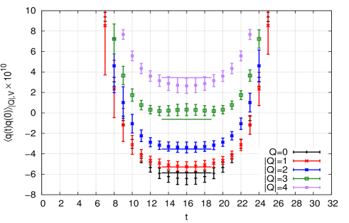
Figure 1: $\langle q(t)q(0)\rangle_{|Q|,V}$ as a function of the separation $t$ at flow time $\tau=6\tau_{0}$ for different values of the topological charge $Q$. The horizontal lines are the expected plateaus $-(\chi_{t}/V)(1-Q^{2}/(\chi_{t}V))$ with $\chi_{t}a^{4}=7.76\times 10^{-5}$ from Section 2.

The theoretically expected values, using $\chi_{t}a^{4}=7.76(20)\times 10^{-5}$ from the previous section, have also been plotted and are represented by the horizontal lines. The plateau values corresponding to different $Q$, as predicted in eq. (2), are clearly distinct. For values with $Q^{2}/(\chi_{t}V)\ll 1$ (i.e. $|Q|\leq 2$), there is excellent agreement. On the other hand, for $|Q|\geq 3$ there is a slight tension, probably a consequence of $Q^{2}/(\chi_{t}V)\geq 0.88$, which is the expansion parameter of eq. (2) and which should be small. We obtain $\chi_{t}a^{4}=7.69(22)\times 10^{-5}$ via a combined fit to the $Q=0$, $|Q|=1$ and $|Q|=2$ results, which is consistent with our unfixed topology result from Section 2, $\chi_{t}a^{4}=7.76(20)\times 10^{-5}$.

4 Computation of $\chi_{t}$ with the slab method

Assuming a Gaussian distribution of the topological charge, this method uses spacetime subvolumes $xV$, $x\in[0,1]$ called “slabs”. The probability of having topological charge $\bar{Q}\in\mathbb{R}$ inside a slab under the condition that the topological charge of the total volume is $Q$ is straightforward to calculate,

$$p(\bar{Q})p(Q-\bar{Q})\bigg{|}_{xV,Q}\propto\exp\bigg{(}-\frac{\bar{Q}^{2}}{2\chi_{t}Vx}\bigg{)}\times\exp\bigg{(}-\frac{(Q-\bar{Q})^{2}}{2\chi_{t}V(1-x)}\bigg{)}.$$ (3)

Defining $\bar{Q}^{\prime}=\bar{Q}-xQ$ allows to simplify (3),

$$p(\bar{Q})p(Q-\bar{Q})\bigg{|}_{xV,Q}\propto\exp\bigg{(}-\frac{\bar{Q}^{\prime 2}}{2\chi_{t}Vx(1-x)}\bigg{)}.$$ (4)

From this expression one can read off

$$\Big{\langle}\bar{Q}^{\prime 2}\Big{\rangle}=\chi_{t}Vx(1-x).$$ (5)

The method to extract the topological susceptibility is then straightforward: one has to compute $\langle\bar{Q}^{\prime 2}\rangle$, the average of $\bar{Q}^{\prime 2}$ on the available gauge link configurations with topological charge $Q$, for several values of $x$. The resulting points should be consistent with the parabola (5), i.e. $\chi_{t}$ can be obtained with a corresponding fit.

In Fig. 2, numerical results for $\langle\bar{Q}^{\prime 2}\rangle$ are shown for $|Q|=0,1,2$.

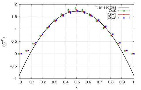
Figure 2: $\langle\bar{Q}^{\prime 2}\rangle$ as a function of $x$ for different values of the topological charge $Q$ (for better visibility points for $Q=0$ ($|Q|=2$) are slightly shifted to the left (right)). The black curve represents the fit of eq. (5) with an additive constant to the data points.

The slabs used for the computations have temporal extent $xT$ and spatial volume $L^{3}$, periodic in space. We observe that the data points are not fully consistent with the quadratic curve (5). In particular at small $x$ and small $1-x$ there are strong discrepancies. On the other hand, the data points in the interval $0.2\leq x\leq 0.8$ can be described nicely with (5), if one allows for an additive constant. Moreover, the corresponding result, $\chi_{t}a^{4}=7.63(14)\times 10^{-5}$, is then in agreement with the unfixed topology result from Section 2, $\chi_{t}a^{4}=7.76(20)\times 10^{-5}$. The distortions at small $x$ and small $1-x$ seem to be related to the gradient flow: for large flow times, these distortions become more and more prominent. Understanding this issue in detail is part of our current research.

5 Summary and conclusions

To conclude, we have presented two methods allowing for the extraction of the topological susceptibility from simulations within a single topological sector. We have successfully applied them to QCD, demonstrating their practical use. The slab method has the advantage that one can apply it to any sufficiently large volume without encountering additional problems, while for the AFHO method the signal-to-noise ratio becomes worse when increasing the volume (cf. [8] for a detailed discussion).

References

- [1] M. Lüscher and S. Schaefer, JHEP 1107, 036 (2011) [arXiv:1105.4749 [hep-lat]].
- [2] S. Aoki et al., PTEP 2012, 01A106 (2012).
- [3] K. Cichy, G. Herdoiza and K. Jansen, Nucl. Phys. B 847, 179 (2011) [arXiv:1012.4412 [hep-lat]].
- [4] H. Fukaya, S. Hashimoto, T. Hirohashi, K. Ogawa and T. Onogi, Phys. Rev. D 73, 014503 (2006) [hep-lat/0510116].
- [5] W. Bietenholz et al., JHEP 0603, 017 (2006) [hep-lat/0511016].
- [6] F. Bruckmann et al., Eur. Phys. J. A 43, 303 (2010) [arXiv:0905.2849 [hep-lat]].
- [7] S. Aoki, H. Fukaya, S. Hashimoto and T. Onogi, Phys. Rev. D 76, 054508 (2007) [arXiv:0707.0396 [hep-lat]].
- [8] I. Bautista et al., Phys. Rev. D 92, 114510 (2015) [arXiv:1503.06853 [hep-lat]].
- [9] P. de Forcrand et al., Nucl. Phys. Proc. Suppl. 73, 578 (1999) [hep-lat/9810033].
- [10] W. Bietenholz, P. de Forcrand and U. Gerber, JHEP 1512, 070 (2015) [arXiv:1509.06433 [hep-lat]].
- [11] K. Jansen and C. Urbach, Comput. Phys. Commun. 180, 2717 (2009) [arXiv:0905.3331 [hep-lat]].
- [12] W. Bietenholz et al., arXiv:1603.05630 [hep-lat].