On the maximum Lyapunov exponent of the motion in a chaotic layer

Abstract

The maximum Lyapunov exponent (referred to the mean half-period of phase libration) of the motion in the chaotic layer of a nonlinear resonance subject to symmetric periodic perturbation, in the limit of infinitely high frequency of the perturbation, has been numerically estimated by two independent methods. The newly derived value of this constant is $0.80$, with precision presumably better than $0.01$.

1 Introduction

On the basis of results of extended numerical experiments, Chirikov C78 ; C79 noted that the maximum Lyapunov exponent, referred to the mean half-period of phase libration, of the motion in the chaotic layer of a nonlinear resonance subject to symmetric periodic perturbation, is approximately constant in a wide range of a parameter characterizing the perturbation frequency. In this paper, we estimate the least upper bound for the maximum Lyapunov exponent of the separatrix map. We show that this bound coincides with the value of the maximum Lyapunov exponent in the mentioned problem in the limit of infinitely high frequency of perturbation, and its value does not depend on the amplitude of the perturbation, i. e. it is defined robustly. In what follows, this quantity is called Chirikov’s constant. The knowledge of the value of Chirikov’s constant is important for accurate analytical estimation of Lyapunov exponents in applications in mechanics and physics S00a ; S02 .

Nonlinear resonances are ubiquitous in problems of modern mechanics and physics. Under general conditions C77 ; C79 ; LL92 , a model of a nonlinear resonance is provided by the nonlinear pendulum with periodic perturbations. The rigid pendulum with the oscillating suspension point is a paradigm in studies of nonlinear resonances and chaotic behavior in Hamiltonian dynamics. The Hamiltonian of this system, according to e. g. BM95 , is:

$$H={{{\cal G}p^{2}}\over 2}-{\cal F}\cos\varphi+a\left(\cos(\varphi-\tau)+\cos(\varphi+\tau)\right),$$ (1)

where $\tau=\Omega t+\tau_{0}$. The first two terms in Eq. (1) represent the Hamiltonian $H_{0}$ of the unperturbed pendulum, while the two remaining ones the periodic perturbations. The variable $\varphi$ is the pendulum angle (this angle measures deviation of the pendulum from the lower position of equilibrium), and $\tau$ is the phase angle of perturbation. The quantity $\Omega$ is the perturbation frequency, and $\tau_{0}$ is the initial phase of the perturbation; $p$ is the momentum; ${\cal F}$, ${\cal G}$, $a$ are constants. In what follows, it is assumed that ${\cal F}>0$, ${\cal G}>0$.

Chirikov C77 ; C79 derived the so-called separatrix map describing the motion in the vicinity of the separatrices of Hamiltonian (1):

$$w_{i+1}=w_{i}-W\sin\tau_{i},$$

$$\tau_{i+1}=\tau_{i}+\lambda\ln{32\over|w_{i+1}|}\ \ \ (\mbox{mod }2\pi),$$ (2)

where $w$ denotes the relative (with respect to the separatrix value) pendulum energy $w={H_{0}\over{\cal F}}-1$, and $\tau$ retains its meaning of the phase angle of perturbation. Constants $\lambda$ and $W$ are parameters: $\lambda$ is the ratio of $\Omega$, the perturbation frequency, to $\omega_{0}=({\cal FG})^{1/2}$, the frequency of the small-amplitude pendulum oscillations; and

$$W={a\over{\cal F}}\lambda(A_{2}(\lambda)+A_{2}(-\lambda))=4\pi{a\over{\cal F}}\lambda^{2}\mbox{csch}{\pi\lambda\over 2},$$ (3)

where

$$A_{2}(\lambda)=4\pi\lambda{\exp{\pi\lambda\over 2}\over\sinh(\pi\lambda)}$$ (4)

is the Melnikov–Arnold integral C79 ; LL92 ; S98a . One iteration of map (2) corresponds to one period of the pendulum rotation, or a half-period of its libration. The motion of system (1) is mapped by Eqs. (2) asynchronously S98a : the action-like variable $w$ is taken at $\varphi=\pm\pi$, while the perturbation phase $\tau$ is taken at $\varphi=0$. The desynchronization can be removed by a special procedure S98a ; S00 .

An equivalent form of Eqs. (2), used e. g. in CS84 , is

$$y_{i+1} = y_{i}+\sin x_{i},$$

$$x_{i+1} = x_{i}-\lambda\ln|y_{i+1}|+c\ \ \ (\mbox{mod }2\pi),$$ (5)

where $y={w\over W}$, $x=\tau+\pi$; and the new parameter

$$c=\lambda\ln{32\over|W|}.$$ (6)

The standard map represents linearization of the separatrix map in the action-like variable $y$ near a fixed point; it is given by the equations

$$y_{i+1} = y_{i}+K\sin x_{i}\ \ \ (\mbox{mod }2\pi),$$

$$x_{i+1} = x_{i}+y_{i+1}\ \ \ (\mbox{mod }2\pi),$$ (7)

where $K$ is the so-called stochasticity parameter C78 ; C79 .

2 The Lyapunov exponents and the dynamical entropy

The calculation of the Lyapunov characteristic exponents (LCEs) is one of the most important tools in the study of the chaotic motion. The LCEs characterize the rate of divergence of trajectories close to each other in phase space. A nonzero LCE indicates chaotic character of motion, while the maximum LCE equal to zero is the signature of regular (periodic or quasi-periodic) motion. The quantity reciprocal to the maximum LCE characterizes the motion predictability time.

Let us consider two trajectories close to each other in phase space. One of them we shall refer to as guiding and the other as shadow. Let $d(t_{0})$ be the length of the displacement vector directed from the guiding trajectory to the shadow one at an initial moment $t=t_{0}$. The LCE is defined by the formula LL92 :

$$L=\limsup_{{t\to\infty}\atop{d(t_{0})\to 0}}{1\over{t-t_{0}}}\ln{d(t)\over d(t_{0})}\,.$$

In the case of a Hamiltonian system, the quantity $L$ may take $2N$ different values (depending on the direction of the initial displacement), where $N$ is the number of degrees of freedom; the LCEs divide into pairs: for each $L_{k}>0$ there exists $L_{k+N}=-L_{k}<0$, $k=1,\ldots,N$.

The LCEs are closely related to the dynamical entropy P76 ; BGS76 ; C78 ; C79 ; M92 . For the Hamiltonian systems with 3/2 and 2 degrees of freedom, Benettin et al. proposed the relation $h=L\mu$ (BGS76, , Eq. (6)), where $h$ is the dynamical entropy, $L$ is the maximum LCE, and $\mu$ is the relative measure of the connected chaotic domain where the motion takes place. This formula is approximate. Benettin et al. BGS76 applied it in a study of the chaotic motion of the Hénon–Heiles system.

In what follows, our numerical data is presented on the measure $\mu$ of the main connected chaotic domain in phase space of the standard map, the maximum LCE $L$, and the product of $\mu$ and $L$ for motion in this domain. Two methods for computation of the chaotic domain measure $\mu$ are used. A traditional “one trajectory method” (OTM) consists in computing the number of cells explored by a single trajectory on a grid exposed on phase plane. A “current LCE segregation method” (CLSM) is based on an analysis of the differential distribution of the computed values of the Lyapunov exponents (current LCEs) of a set of trajectories with starting values on a grid on phase plane. Both methods were proposed and used by Chirikov C78 ; C79 in computations of $\mu$ for the standard map. Analogous methods were used in SM03 in computations of chaotic domain measure in the Hénon–Heiles problem.

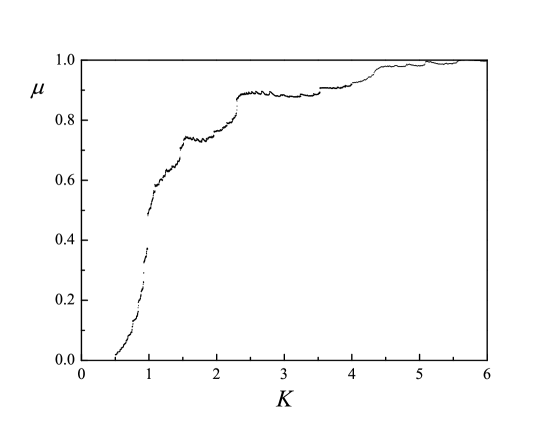
(b) 

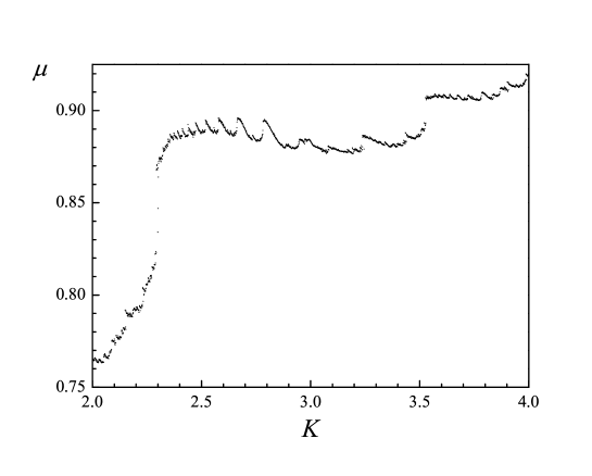
Figure 1: The dependence $\mu(K)$ (a); a detail enlarged (b)

Fig.1 illustrates discontinuity of the obtained $\mu(K)$ function. The curve in Fig.1 is obtained by the OTM on the grid $2000\times 2000$ pixels on phase plane ($x$, $y$) $\in[0,2\pi]\times[0,2\pi]$, the number of iterations $n_{it}=10^{8}$. A prominent bump in the dependence, shown in detail in Fig.1b, is conditioned by the process of desintegration of the half-integer resonance in the course of a sequence of period-doubling bifurcations while $K$ is increasing from $\approx 2$ to $\approx 2.5$. A similar but less pronounced bump is seen in Fig.1a in the range $4<K<4.5$; this one is due to bifurcations of the integer resonance.

In general, at these moderate values of $K$ (at $K<6$), the discontinuities are conditioned by the process of absorption of minor chaotic domains by the main chaotic domain, while $K$ increases.

In Fig.2, we give the plot of the maximum LCE and the dynamical entropy in a broad range of $K$. Each value of $L$ in Fig.2 represents the mean value of the maximum LCEs over 10 trajectories of length $n_{it}=10^{7}$ each. The initial data for these trajectories slightly differ from each other, but in all cases are chosen to lie inside the main chaotic domain. Everywhere in this work (including the case of the separatrix maps considered below) the presented values of LCEs have been computed by the tangent map method described e. g. in C78 ; C79 .

The corresponding dependence of $h=L\mu$ on $K$ is plotted in Fig.2; the values of $\mu$ obtained by the OTM (Fig.1) have been used. One can see that our numerical experiments suggest that the dynamical entropy of the standard map is continuous and monotonous in $K$, contrary to the discontinuous behavior of LCEs. This is no wonder, since the dynamical entropy is a more fundamental quantity.

For orientation, the function $\ln{K\over 2}$ is depicted in the same Fig.2; this is the well-known logarithmic law derived by Chirikov C78 ; C79 analytically by means of averaging the largest eigenvalue of the tangent map in assumption that the relative measure of the regular component is small.

The downward spikes seen in the $L(K)$ dependence in Fig.2 (and in Fig.3 also) represent a manifestation of the so-called “stickiness effect” immanent to the chaotic Hamiltonian dynamics in conditions of divided phase space S98b : a chaotic trajectory may stick for a long time to the borders of the chaotic domain, where the motion is close to regular, and therefore the local LCEs are small. Since the computation time is always finite, the stickiness effect, in the case of deep stickings, leads to underestimated values of LCEs; see discussion in S98b .

The $L(K)$ and $\mu(K)$ functions are discontinuous and evidently elude simple analytic representation in broad ranges of $K$. The case of $h(K)$ is different. With good accuracy, the numerical dependence at $K$ greater than its critical value can be approximated by a function which is piecewise linear at moderate values of $K$ (see Fig.2), and logarithmic with a small power-law correction at higher values of $K$: $h(K)=\ln{K\over 2}+{1\over K^{2}}$, if $K>4.5$, with accuracy better than $0.01$ in absolute magnitude. So, the presented numerical data indicates that the high-$K$ asymptotics of the $h(K)$ function contains a power-law component, in addition to the well-known logarithmic one. The same is valid for the $L(K)$ dependence, if one ignores the small (and local in $K$) distortions of the function due to accelerator modes and periodic solutions of higher orders.

Let us consider in more detail the accuracy of the presented results. The LCE values can be effectively verified by controlling their saturation, taking various values of $n_{it}$. We compare the maximum LCEs computed taking $n_{it}=10^{7}$ with those computed taking the number of iterations ten times less, $n_{it}=10^{6}$. In both cases we average over ten trajectories. One finds that the difference between the LCEs in these two cases, averaged over the interval $1\leq K<2$ (the step in $K$ is $0.01$, so, $100$ differences are averaged), is equal to only $0.0015$. The saturation is faster with increasing $K$. Therefore the saturation at $n_{it}=10^{7}$ is practically complete at $K>1$, and therefore there are no significant systematic errors in determination of LCEs at such values of $K$.

The problem of accuracy of computation of $\mu$ is more difficult. The generic border of chaos in phase space of Hamiltonian systems is fractal UF85 ; C90 . Umberger and Farmer UF85 conjectured and numerically verified that the coarse-grained measure of the chaotic constituent of phase space of two-dimensional area-preserving maps scales with the grid resolution $\varepsilon$, employed to estimate the measure, as a power law in the limit $\varepsilon\to 0$:

$$\mu_{\varepsilon}=\mu_{0}+A\varepsilon^{\beta},$$ (8)

where $\mu_{0}$ is the actual measure, $A$ and $\beta$ are constants characterizing the border; $A$, $\beta\geq 0$.

Numerical experiments provide values of $\mu_{\varepsilon}$ for a given $\varepsilon$. So, there are three undetermined quantities in Eq. (8): $\mu_{0}$, $A$, and $\beta$. To obtain their numerical values one needs to compute $\mu_{\varepsilon}$ at least thrice, i. e. at three different resolutions $\varepsilon$ of the grid. Then, the system of three nonlinear equations (8) can be solved. We take three partitions of phase plane of the standard map: $2500\times 2500$, $5000\times 5000$, and $7500\times 7500$ pixels; i. e. $\varepsilon=1/2500$, $1/5000$, and $1/7500$. As in UF85 , the OTM is used; $n_{it}=10^{10}$. The minimum $\varepsilon$ and maximum $n_{it}$ used in UF85 were $1/4096$ and $10^{8}$ respectively. Thus we should expect better estimates of the chaotic domain measure in the present study.

In our numerical experiment, we have computed $\mu_{0}$ and $\beta$ for ten values of $K$ equally spaced in the interval $[1.0,5.5]$, and for ten values of $K$ equally spaced in the interval $[1.0,1.9]$. At all points, the computed value of $\mu_{1/7500}$ ($\mu_{\varepsilon}$ at the smallest $\varepsilon=1/7500$) and the resulting actual $\mu_{0}$ value differ by no more than $0.01$; at $K>1.5$ they coincide with accuracy of two significant digits.

Our data for $K=1.1$, $1.2$, and $1.3$ can be compared to results by Umberger and Farmer UF85 , who computed the chaotic domain measure for these three values of $K$. The difference in their and our values of $\mu_{0}$ does not exceed $\approx 0.01$. Our results on the chaotic domain measure are as well in reasonable agreement with early estimates by Chirikov C78 ; C79 . The close proximity of the values of $\mu_{0}$ to those of $\mu_{1/7500}$, as well as the agreement of them with the results C78 ; C79 ; BGS76 , testify that our estimates of the chaotic domain measure have the accuracy better than $0.01$.

The power-law index $\beta$ is related to the fractal dimension $d_{L}$ of the set of all chaos borders inside the connected chaotic domain C90 : $d_{L}=2-\beta$. From our data, one has $\langle\beta\rangle=0.63\pm 0.13$, and $d_{L}\approx 1.37\pm 0.13$. This agrees well with the theoretical estimate $d_{L}=3/2$ by Chirikov C90 .

An important constant of the standard map dynamics is the chaotic domain measure at the critical value of the stochasticity parameter $K=K_{G}=0.971635406\ldots$ (on the critical value, see e. g. M92 ). Our calculation performed by the same algorithm as presented above gives $\mu(K_{G})\approx 0.463$. The contribution of the chaotic domain around the integer resonance to this quantity is $3.5$ times greater than that of the half-integer one ($0.463\approx 0.359+0.103$). The calculated values of the parameter $\beta$ in these domains are equal to $\approx 0.53$ and $\approx 0.49$ respectively; so, the border fractal dimension $d_{L}=2-\beta$ in the critical case $K=K_{G}$ is particularly close, as one could expect, to the theoretical estimate $d_{L}=3/2$ by Chirikov C90 .

3 Estimation of Chirikov’s constant

The value of Chirikov’s constant can be found by calculating the average of the local maximum LCE over the chaotic layer of map (5) in the limit $\lambda\to\infty$. The local LCE must be taken with weight directly proportional to the time that the trajectory spends in a given part of the layer; this time is directly proportional to the local relative measure of the chaotic component. Therefore one has the following formula

$$C_{h}=\lim_{\lambda\to\infty}\frac{\int\limits_{0}^{y_{b}}\tilde{L}_{sx}(y)\tilde{\mu}_{sx}(y)\,dy}{\int\limits_{0}^{y_{b}}\tilde{\mu}_{sx}(y)\,dy},$$ (9)

where $y_{b}=\lambda/K_{G}$ is the value of $y$ at the border of the layer, $\tilde{L}_{sx}(y)$ is the local (with respect to $y$) value of the maximum LCE of the separatrix map, and $\tilde{\mu}_{sx}(y)$ is the local chaos measure. The tilde cap marks that the quantities are local. This formula is valid in the limit $\lambda\to\infty$, since only in this limit one can reduce the sum over all integer resonances inside the layer to an integral. What is more, the formula $y_{b}=\lambda/K_{G}$ (see C90 ; S98a ) is accurate also only in this limit.

By means of the substitution $y=\lambda/K$ we introduce a new independent variable $K$, which is nothing but the value of the stochasticity parameter of the standard map locally approximating the separatrix map. The accuracy of the approximation improves with increasing $\lambda$ C78 ; C79 , i. e. the local characteristics of the chaotic layer converge to those of the standard map locally approximating the motion: $\tilde{L}_{sx}(y=\lambda/K)\to L(K)$ and $\tilde{\mu}_{sx}(y=\lambda/K)\to\mu(K)$, where $L(K)$ and $\mu(K)$ are the maximum LCE and the measure of the main connected chaotic domain of the standard map in function of $K$. The dependence on $\lambda$ in the limit $\lambda\to\infty$ is eliminated, and Eq. (9) is reduced to the final form:

$$C_{h}=\frac{K_{G}}{\sigma}\int\limits_{K_{G}}^{\infty}L(K)\mu(K)\,\frac{dK}{K^{2}}\,,$$ (10)

where the quantity

$$\sigma=\lim_{\lambda\to\infty}y_{b}^{-1}\int\limits_{0}^{y_{b}}\tilde{\mu}_{sx}(y)\,dy=K_{G}\int\limits_{K_{G}}^{\infty}\mu(K)\,\frac{dK}{K^{2}}$$ (11)

has the meaning of “porosity” of the chaotic layer. This is the ratio of the area of the chaotic component to the total area of the layer bounded by its external borders; the quantity $1-\sigma$ is nothing but the total relative area of all regular islands inside the layer.

For $K\in[K_{G},10]$, we integrate Eqs. (10, 11) numerically; the functions $L(K)$ and $\mu(K)$ are taken in numerical form, as presented in Figs. 1 and 2. The remainders for $K>10$ are calculated analytically, with $h(K)=L(K)\mu(K)$ set equal to $\ln{K\over 2}+{1\over K^{2}}$ (as established above), and $\mu(K)$ set equal to unity. Adopting accuracy of two significant digits, one has $C_{h}=0.80$, $\sigma=0.78$.

Our value of $C_{h}$ differs significantly from the value of $0.663$ got by Chirikov by integration of the dynamical entropy of the standard map in C78 ; C79 (where $C_{h}$ is designated as $h_{W}$). This deviation is due to the sparsity of the numerical data obtained more than twenty years ago, as well as to ignoring the porosity of the chaotic layer in an approximate calculation in C78 ; C79 .

As discussed in the previous Section, the numerical dependence $\mu(K)$ is less certain than $L(K)$. Hence its uncertainty is the most likely source of errors in estimating $C_{h}$. The estimated error in determination of $\mu(K)$ does not exceed $0.01$ (see above). At high values of $K$ (at $K>6$), the deviations are much less than $0.01$, because $\mu(K)$ rapidly converges to unity. To estimate the accuracy of the obtained value of $C_{h}$, we recompute this value substituting $\mu(K)\pm 0.01$ instead of the original $\mu(K)$ in Eqs. (10) and (11) at $K\leq 10$ (if $\mu(K)+0.01>1$ we set $\mu(K)=1$, of course). We find that both these negative and positive shifts in $\mu(K)$ change the resulting value of $C_{h}$ by no more than $0.004$. Therefore, if one takes three significant digits in $C_{h}$, the result is $C_{h}=0.801\pm 0.004$ in the described sense. The deviations in $\sigma$ are greater: $\sigma=0.780\pm 0.009$. Finally, rounding up, we conclude that the accuracy of our estimate $C_{h}=0.80$ is presumably better than $0.01$.

One can verify this estimate of Chirikov’s constant by means of a straightforward computation of the maximum LCE of the separatrix map at high values of $\lambda$. The $\lambda$ dependence of the maximum LCE of the separatrix map is shown in Fig.3. It has been obtained by a numerical experiment with map (5). The use of one and the same designation $L$ for the LCE in the both cases of the standard and separatrix maps should not cause confusion. The resolution (step) in $\lambda\in[0,10]$ is equal to $0.05$. At each step in $\lambda$, the values of $L$ have been computed for 100 values of $c$ equally spaced in the interval $[0,2\pi]$. The number of iterations for each trajectory is $n_{it}=10^{7}$ for $\lambda\in[0,1)$ and $n_{it}=10^{8}$ for $\lambda\in[1,10]$ (the saturation time for numerical estimates of LCEs increases with $\lambda$, and therefore more computational time is needed to get reliable values of LCEs at high values of $\lambda$). This is sufficient to saturate the computed values of $L$; see below. At each step in $\lambda$ we find the value of $c$ corresponding to the minimum width of the layer (the case of the least perturbed border), and plot the value of $L$ corresponding to this case. The case of the least perturbed border is generic in applications, in the sense that strong perturbations of the border are local in $c$. Note that the parameter $c$ is related to the amplitude of the periodic perturbation in Hamiltonian (1) at a given value of $\lambda$ by Eq. (6).

Fig.3 also presents approximation of the observed dependence by the rational function

$$L(\lambda)={b+c\lambda\over 1+a\lambda}$$ (12)

with $b$ set to zero in order that $L(0)=0$. The resulting values of the parameters and their standard errors are: $a=2.097\pm 0.033$, $b=0$, and $c=1.691\pm 0.024$.

Chirikov’s constant is given by the limit $L(\lambda\to\infty)$; so, according to the described numerical experiment, $C_{h}\approx 0.806$, in good agreement with the result presented above ($C_{h}\approx 0.801$).

The integration time we used is sufficient for effective saturation of the computed LCE in the given interval of $\lambda$. Indeed, setting $n_{it}=10^{7}$ for the whole interval $\lambda\in[0,10]$ gives the resulting $C_{h}\approx 0.808$, i. e. the resulting $C_{h}$ value is negligibly different from the value obtained with $n_{it}$ raised to $10^{8}$ at $\lambda\in[1,10]$.

Variation of the parameter $c$ in map (5) produces a scatter in the computed values of LCE, due to emergence and disappearance of marginal resonances at the border of the chaotic layer (on the marginal resonances see S98a ). Let us prove that the LCE scatter tends to zero in the limit $\lambda\to\infty$; in other words, the limit of LCE is one and the same for all (though sufficiently small, for the map description to be valid) amplitudes of perturbation.

The largest variations are conditioned by integer marginal resonances. The $y$ coordinates of the centers of the integer resonances satisfy the relation $y_{i+1}/y_{i}=\exp(2\pi/\lambda)$, where $i$ is the number of the resonance. This relation follows from the second line of map (5). At the border of the layer $y\approx\lambda$ (see C78 ; C79 ); therefore in the case of $\lambda\gg 1$ the distance between the centers of two consecutive integer resonances at the border is $\Delta y\approx 2\pi$. The relative local measure $\mu_{marg}$ of the chaotic component associated with the separatrices of a marginal resonance depends on the value of the parameter $K$ of the standard map locally approximating the motion near the marginal resonance; the maximum value is $\approx 0.46$ at $K=K_{G}$ (see the concluding paragraph of Section 2), because any marginal resonance has $K<K_{G}$. This relative measure referred to the total chaotic measure of the layer is less than approximately $(\mu_{marg}\cdot 2\pi)/(\sigma\cdot\lambda)\approx 3.7/\lambda$. The largest value of the local LCE at the border is again associated with $K=K_{G}$; it equals approximately $0.11$ (see Fig.2). So, the contribution of the chaotic layer of the marginal resonance to the total value of the maximum LCE over the whole layer varies from zero up to $\approx 0.4/\lambda$, depending on the prominence of the marginal resonance, i. e. on the local value of $K$ at the border. This contribution tends to zero with $\lambda\to\infty$, and therefore the value of Chirikov’s constant does not depend on the second parameter of the separatrix map, $c$, and consequently on the amplitude of the periodic perturbation.

4 Conclusions

Exploiting our high-precision data on the functions $h(K)$ and $\mu(K)$, we have calculated the value of Chirikov’s constant $C_{h}$ — the least upper bound for the maximum Lyapunov exponent of the separatrix map. This quantity is nothing but the maximum Lyapunov exponent (referred to the mean half-period of phase libration, or, equivalently, to the mean period of phase rotation) of the motion in the chaotic layer of a nonlinear resonance subject to symmetric periodic perturbation, in the limit of infinitely high frequency of the perturbation. We have shown that the value $C_{h}$ does not depend on the second parameter of the separatrix map (or, equivalently, on the amplitude of the perturbation).

The newly derived value of $C_{h}$ is $0.80$, with precision presumably better than $0.01$. The knowledge of this constant is important for correct analytical estimation of the value of the maximum Lyapunov exponent of the chaotic motion of a Hamiltonian system allowing description in the perturbed pendulum model.

The author is thankful to B. V. Chirikov and V. V. Vecheslavov for valuable discussions. This work was supported by the Russian Foundation for Basic Research (project number 03-02-17356).

(a) 

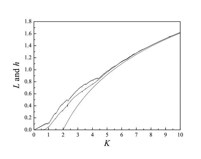
Figure 2: $L(K)$ (the uppermost curve), $h(K)$, and $\ln{\frac{K}{2}}$ in a broad range of $K$

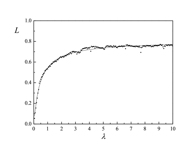
Figure 3: The dependence $L(\lambda)$ for the separatrix map (the case of the least perturbed border of the chaotic layer) and its rational approximation

References

- (1) B. V. Chirikov, Interaction of Nonlinear Resonances (Novosib. Gos. Univ., Novosibirsk, 1978). In Russian.
- (2) B. V. Chirikov, Phys. Rep. 52, 263 (1979).
- (3) I. I. Shevchenko, Izvestia GAO 214, 153 (2000). In Russian.
- (4) I. I. Shevchenko, Kosmicheskie Issledovaniya 40, 317 (2002) [Cosmic Res., 40, 296 (2002)].
- (5) B. V. Chirikov, Nonlinear Resonance (Novosib. Gos. Univ., Novosibirsk, 1977). In Russian.
- (6) A. J. Lichtenberg and M. A. Lieberman, Regular and Chaotic Dynamics (Springer-Verlag, New York, 1992; Mir, Moscow, 1984).
- (7) B. S. Bardin and A. P. Markeev, Prikl. Mat. Mekh. 59, 922 (1995). In Russian.
- (8) I. I. Shevchenko, Phys. Scr. 57, 185 (1998).
- (9) I. I. Shevchenko, Zh. Eksp. Teor. Fiz. 118, 707 (2000) [JETP 91, 615 (2000)].
- (10) B. V. Chirikov and D. L. Shepelyansky, Physica D13, 395 (1984).
- (11) Ya. B. Pesin, Doklady Akademii Nauk SSSR 226, 774 (1976). In Russian.
- (12) G. Benettin, L. Galgani, and J. M. Strelcyn, Phys. Rev. A14, 2338, (1976).
- (13) J. D. Meiss, Phys. Rep. 64, 795 (1992).
- (14) I. I. Shevchenko and A. V. Melnikov, Pis’ma Zh. Eksp. Teor. Fiz. 77, 772 (2003) [JETP Letters 77, 642 (2003)].
- (15) I. I. Shevchenko, Phys. Letters A241, 53 (1998).
- (16) D. K. Umberger and J. D. Farmer, Phys. Rev. Letters 55, 661 (1985).
- (17) B. V. Chirikov, INP Preprint 90–109 (1990).
(a)
(b)