See pages - of Schmid_Maintext.pdf

Supporting Information

Schmid et al.

SI Methods

General implementation of semi-ensemble HMM. In the following, we include all formulae required for the implementation of semi-ensemble HMM as demonstrated herein. For more general introductions to HMM, please refer to the respective literature (14,15).
Forward-Backward, Baum-Welch and Viterbi algorithms were implemented for continuous observables and multiple dimensions. Numerical underflow or overflow is prevented by logarithmic renormalization. Recursive calculations are sped up by multi-threading (processing several time-traces in parallel). All software was written in IgorPro v6.3 (Wavemetrics) and calculations were run on an iMac (Apple, 2014, 2.9 GHz Intel i5 processor, 16GB RAM) or a comparable Windows PC. A typical optimization (4 states, >100 traces) took less than an hour.

HMM conventions and parameters. The indices $i,j$ denote states. $t$ are discrete time steps and $T$ is the total time of a trajectory. $O$ is the set of observables and $\bm{x}_{t}$ is a specific observable at time $t$ in $d$ dimensions (herein $d=2$ for donor and acceptor fluorescence). The complete set of parameters, $\lambda(\bm{\pi},\bf A,B)$, consists of:

$$\pi_{i} \overset{\scriptscriptstyle\wedge}{=}\text{start probabilites}$$

$$a_{ij} \overset{\scriptscriptstyle\wedge}{=}\text{transition probabilities}$$

$$b_{i}(\bm{\mu}_{i},V_{i}) \overset{\scriptscriptstyle\wedge}{=}\text{Gaussian emission probability densities}$$

with means $\bm{\mu}_{i}$ and covariance matrix $V_{i}$ , both in $d$ dimensions. TIRF data is appropriately described by Gaussian emissions (in place of Poissonian), because each time bin contains much more than ten photons including noise. $b_{i}(\bm{x}_{t})$ denotes the emission density value for a specific observable value at a given time t (scalar, may be >1).

Implementation of the forward-backward algorithm. The forward and backward variables, $\alpha$ and $\beta$, are auxiliary probabilities prerequisite for the Baum-Welch algorithm below.

initiation: $$\alpha_{t=1}(i) =\pi_{i}\,b_{i}(\bm{x}_{t=1})$$

recursion: $$\alpha_{t+1}(i) =\sum_{j}\left[\alpha_{t}(j)\,a_{ji}\right]\,b_{i}(\bm{x}_{t+1})$$

termination: $$P(O|\lambda) =\sum_{i}\alpha_{T}(i)$$

initiation: $$\beta_{T}(i) =1$$

recursion: $$\beta_{t}(i) =\sum_{j}a_{ij}\,b_{j}(\bm{x}_{t+1})\,\beta_{t+1}(j)$$

termination: $$P(O|\lambda) =\sum_{i}\pi_{i}\,b_{i}(\bm{x}_{1})\,\beta_{t=1}(i)$$

$P(O|\lambda)$ is called the production probability of the data given the model. It is equivalent to the likelihood of the model given the data $\mathcal{L}(\lambda|O)$.

Implementation of the Baum-Welch algorithm. The basis for calculating the updated parameters are $\gamma_{t}(i)$ and $\gamma_{t}(i,j)$, the respective probabilities for a given state or transition at a given time point.

$$\gamma_{t}(i) =\alpha_{t}(i)\,\beta_{t}(i)/P(O|\lambda)$$

$$\gamma_{t}(i,j) =\alpha_{t}(i)\,a_{ij}\,b_{j}(\bm{x}_{t+1})\,\beta_{t+1}(j)/P(O|\lambda)$$

The parameter update equations are:

$$\hat{\pi}_{i} =\gamma_{t=1}(i)$$

$$\hat{a}_{ij} =\sum\nolimits_{t=1}^{T-1}\left[\gamma_{t}(i,j)\right]/\sum\nolimits_{t=1}^{T-1}\gamma_{t}(i)$$

$$\hat{\bm{\mu}}_{i} =\sum\nolimits_{t=1}^{T}\left[\gamma_{t}(i)\,\bm{x}_{t}\right]/\sum\nolimits_{t=1}^{T}\gamma_{t}(i)$$

$$\hat{V}_{i} =\sum\nolimits_{t=1}^{T}\left[\gamma_{t}(i)\,\bm{x}_{t}\,{\bm{x}_{t}}^{\mathsf{T}}\right]/\sum\nolimits_{t=1}^{T}\left[\gamma_{t}(i)\right]-\bm{\mu}_{i}\,{\bm{\mu}_{i}}^{\mathsf{T}}$$

The ensemble parameters $\Pi_{i}$, $\mathcal{A}_{ij}$ are updated based on all $N$ time-traces:

$$\hat{\Pi}_{i} =\sum\nolimits_{n=1}^{N}\left[{}^{n}\pi_{i}\right]/N$$

$$\hat{\mathcal{A}}_{ij} =\sum\nolimits_{n=1}^{N}\Big{[}\sum\nolimits_{t=1}^{T-1}\left[{}^{n}\gamma_{t}(i,j)\right]\Big{]}/\sum\nolimits_{n=1}^{N}\Big{[}\sum\nolimits_{t=1}^{T-1}\left[{}^{n}\gamma_{t}(i)\right]\Big{]}$$

Implementation of the FRET-constraint. In a true FRET time-trace, the total fluorescence $I_{tot}$ (i.e. the sum of the corrected acceptor and donor signals, ${{}^{A}{x}_{t}}$ and ${{}^{D}{x}_{t}}$, with respective means ${}^{A}\mu_{i}$ and ${}^{D}\mu_{i}$) must remain constant in each state:

$$\langle I_{tot}\rangle=\sum\nolimits_{t=1}^{T}\big{[}{{}^{A}{x}_{t}}+{{}^{D}{x}_{t}}\big{]}/T={{}^{A}\mu_{i}}+{{}^{D}\mu_{i}} =const.\quad\forall\,i$$

This physical constraint is introduced into Baum’s optimization formalism using Lagrange multipliers. Because the resulting update equations for Gaussian distributions are coupled in $\bm{\mu}_{i}$ and $V_{i}$, we exploit the fact that the difference between Gaussian and Poissonian means is negligible for TIRF signals. Therefore, the update equation for constrained Poissonian distributions (35) can be utilized to optimize $\bm{\mu}_{i}$ :

$$\hat{\bm{\mu}}_{i} =\langle I_{tot}\rangle\cdot\sum\nolimits_{t=1}^{T}\left[\gamma_{t}(i)\,\bm{x}_{t}\right]/\sum\nolimits_{t=1}^{T}\left[\gamma_{t}(i)\cdot(^{A}{x}_{t}+{{}^{D}}{x}_{t})\right]$$

Implementation of the Viterbi algorithm. The most probable state sequence $s^{*}$ with maximal production probability $P^{*}(O|\lambda)$ is deduced from the $\delta$ and $\psi$ variables.

initiation: $$\delta_{t=1}(i) =\pi_{i}\,b_{i}(\bm{x}_{t=1})$$

recursion: $$\delta_{t+1}(j) =\max_{i}[\delta_{t}(i)a_{ij}]b_{j}(\bm{x}_{t+1})$$

termination: $$P^{*}(O|\lambda) =P(O,s^{*}|\lambda)=\max_{i}\delta_{T}(i)$$

$$s_{T}^{*} =\underset{j}{\operatorname{argmax}}[\delta_{T}(j)]$$

initiation: $$\psi_{t=1}(i) =0$$

recursion: $$\psi_{t+1}(j) =\underset{i}{\operatorname{argmax}}[\delta_{t}(i)a_{ij}]$$

back-tracking: $$s_{t}^{*} =\psi_{t+1}(s^{*}_{t+1})$$

The Bayesian information criterion (BIC). The BIC (22) selects for a model that describes the data well, while keeping the model complexity moderate. This is achieved by balancing the likelihood $\mathcal{L}(\lambda|O)$ against the number of free parameters $k$, with $n$, the number of data points:

$$\text{BIC}=-2\cdot\ln(\mathcal{L})+k\cdot\ln(n)$$

Its applicability in the context of SMACKS was confirmed using synthetic data of known input models (see below).

Simulations. Discrete state sequences were obtained by a Monte-Carlo simulation based on a given transition matrix: photo-bleaching was included by exponential trace length distributions. For comparison with experimental data, corresponding minimal trace lengths were used (typically 30 data points).
As in the experiment, synthetic data contained Gaussian noise ($\upsigma$=0.3*signal), random offsets ($\pm$0.2*signal), degenerate FRET efficiencies (two low / two high), a sampling rate of 5Hz and a bleach rate of 0.03Hz. See example data in Figure S2.

Confidence Interval For each transition probability $a_{ij}$, the parameter space around the maximum likelihood estimator (MLE) is scanned while keeping the remaining parameters fixed at the MLE. The modified models $\lambda^{\prime}$ are compared to the MLE models $\lambda_{\textrm{MLE}}$ by successive likelihood ratio ($LR$) tests (3,27):

$$LR =2\left(\,\ln[\mathcal{L}(\lambda_{\textrm{MLE}}|O)]-\ln[\mathcal{L}(\lambda^{\prime}|O)]\,\right)$$

$$a_{ij}^{\textrm{CB}} =a^{\prime}_{ij}\quad:\quad LR=\chi^{2}_{0.95\textrm{,df}=1}=3.841$$

The 95% confidence bound (CB) is reached where $LR$ crosses the respective significance level for one degree of freedom (df).

Sample Preparation. Hsp90: Yeast Hsp90 dimers (UniProtKB: P02829) supplied with a C-terminal zipper motif were used to avoid dissociation at low concentrations (13). Previously published cysteine positions (36) allowed for specific labeling with donor (61C) or acceptor (385C) fluorophores (see below). Both constructs were cloned into a pET28b vector (Novagen, Merck Biosciences). They include an N-terminal His-tag followed by a SUMO-domain for later cleavage. The QuickChange Lightning kit (Agilent) was used to insert an Avitag for specific in vivo biotinylation at the C-terminus of the acceptor construct. E.coli BL21star cells (Invitrogen) were co-transformed with pET28b and pBirAcm (Avidity) by electroporation (Peqlab) and expressed according to Avidity’s in vivo biotinylation protocol. The donor construct was expressed in E.coli BL21(DE3)cod+ (Stratagene) for 3h at 37°C after induction with 1mM IPTG at OD₆₀₀=0.7 in LB_Kana. A cell disruptor (Constant Systems Ltd.) was used for lysis. Proteins were purified as published (37) (Ni-NTA, tag cleavage, anion exchange, size exclusion). 95% purity was confirmed by SDS-PAGE. Fluorescent labels (Atto550-, Atto647N-maleimide) were purchased from Atto-tec and coupled to cysteins according to the supplied protocol. Hetero-dimers (acceptor+donor) were obtained by 20min incubation of 1$\upmu$M donor, 0.1$\upmu$M biotinylated acceptor homo-dimers and 2mM ADP in measurement buffer (40mM Hepes, 150mM KCl, 10mM MgCl₂) at 47°C. In this way, predominantly biotinylated hetero-dimers bind to the neutravidin (Thermo Fisher) coated fluid chamber (see below). (Residual homo-dimers will show a specific smFRET signal and are excluded from analysis.)
Holliday junction: DNA-oligos similar to (8) with fluorophores Atto488, Atto550 and Atto647N (Atto-tec) attached were purchased from IBA GmbH. A mixture of 100nM of each DNA-oligo in Tris-buffer (5mM Tris, 5mM NaCl, 20mM MgCl₂, pH 7.5) was heated to 90°C for 10 min and cooled down to 20°C (1°C/min) in a thermocycler (Peqlab). Holliday junctions were measured in Tris-buffer (5mM Tris, 5mM NaCl, 500mM MgCl₂) including 0.1% glucose, 10 U/ml glucose oxidase (Aspergillus niger), 100 U/ml catalase (bovine liver, Calbiochem), 2mM Trolox.
If not stated differently, all chemicals were purchased from Sigma Aldrich.

Single-Molecule Setup & Measurements. TIRF setup: An objective-type TIRF setup was built to measure smFRET. Green and red excitation lasers (532nm, Compass 215M, Coherent and 635nm, Lasiris, Stocker Yale) were aligned, expanded and focused onto the back-focal plane of an apochromat TIRF 100x objective (Nikon, NA=1.49). The collected fluorescence is separated from excitation light by notch filters. Off-axis beams are removed by an optical slit and achromatic slit lenses (achromatic doublets, Qioptiq). Finally donor and acceptor fluorescence is split, spectrally filtered again and individually focused side by side onto the EMCCD (iXonUltra, Andor) by best form silica lenses (Qioptiq). Translation stages (Newport) were used to fine-tune the lens positions. Dichroic mirrors and filters were purchased from AHF analysentechnik AG. Optical mounts, lenses, mirrors and further components were purchased from Thorlabs unless stated differently. Measurements were performed in a PEGylated fluid chamber built from two coverslips and Nescofilm by compression at 70°C. To avoid auto-fluorescence background in the red detection channel a silica coverslip was used (Spectrosil2000, Heraeus, manufactured by UQG Ltd.). The refractive index change (glass: 1.52, silica: 1.46) was adjusted for geometrically. Image acquisition and optical shutters were synchronized by a custom-built electronic circuit and a master trigger to achieve 100ms exposure to each ALEX channel (alternating laser excitation).

Selection & Correction of smFRET Time Traces. We exclude incomplete FRET pairs and photo-physical artifacts, such as blinking, by using ALEX for data acquisition. Selection criteria for single molecule time traces are flat plateaus in all three fluorescence channels (donor and acceptor fluorescence after donor excitation and acceptor fluorescence after acceptor excitation), as well as single step bleaching. Hence, a terminating low FRET region (before photo-bleaching) is no longer rejected. Fluorescence time traces are corrected for background offsets, leakage, direct excitation and the gamma factor (20).

SI Notes

Note 1: Hierarchical search for simplified models. Bruno et al. (23) describe a procedure to deduce the simplest, plausible reaction schemes, from data with multiple open and closed conformations, by comparing models of the canonical “MIR”-form (manifest interconductance rank). We consider a 4-state model with 2 open (o) and 2 closed (c) states (N_o=N_c=2), as previously determined by BIC and the bi-exponential dwell time distributions. First, the interconductance rank (i.e. the number of independent o-c links) is determined. To this end, MIR-form models of rank 1 (linear o-o-c-c) and rank 2 (cyclic -o-o-c-c-) are compared in a likelihood ratio ($LR$) test (likelihood of rank $x$ model, $L_{Rx}$):

$$LR=2\cdot[\ln(L_{R2})-\ln(L_{R1})]\;\begin{cases}≤\chi^{2}_{0.95,df=2}\quad\Rightarrow\textrm{rank 1}\\ >\chi^{2}_{0.95,df=2}\quad\Rightarrow\textrm{rank 2}\end{cases}$$

The null hypothesis (rank 1 model) is rejected if the likelihood ratio exceeds the 95% confidence interval given by the $\chi^{2}$-distribution for 2 degrees of freedom ($df$). (One missing link equals a difference of two transitions.) Second, the number of links $N_{l}$ within this rank R is determined by comparing different schemes by BIC. The number of mathematically identifiable links is limited:

$$N_{l}≤R(N_{o}+N_{c}-R)$$

Models with the same rank and the same number of links are mathematically equivalent and cannot be discerned without further experimental data. For Hsp90, we find a cyclic -o-o-c-c- model in the presence of ATP and linear o-o-c-c models for apo, ADP or AMP-PNP conditions.

Note 2: Expected value of observed energy coupling. Let $\langle N_{ij}^{obs}\rangle$ be the expected number of observations for a given transition, in a dataset with $N_{tot}$ data points. If it is smaller than one, the specific transition cannot be resolved. In this case, $f_{ij}^{\textrm{lost}}$ denotes the factor that is actually lost and the expected value of the observed free energy change $\langle\Delta G_{obs}\rangle$ in units of kT is given by:

$$\langle\Delta G_{obs}\rangle=-\sum_{\begin{subarray}{c}\forall i≠j\\ \textrm{ (cycl.)}\end{subarray}}\ln\left[\frac{a_{ij}/f_{ij}^{\textrm{l}ost}}{a_{ji}/f_{ji}^{\textrm{l}ost}}\right]$$

with:

$$f_{ij}^{\textrm{l}ost}=\begin{cases}\langle N_{ij}^{obs}\rangle=N_{tot}\cdot\pi_{i}\cdot a_{ij}\quad&\forall\;\langle N_{ij}^{obs}\rangle<1\\ \;1\quad&\forall\;\langle N_{ij}^{obs}\rangle≥1\end{cases}$$

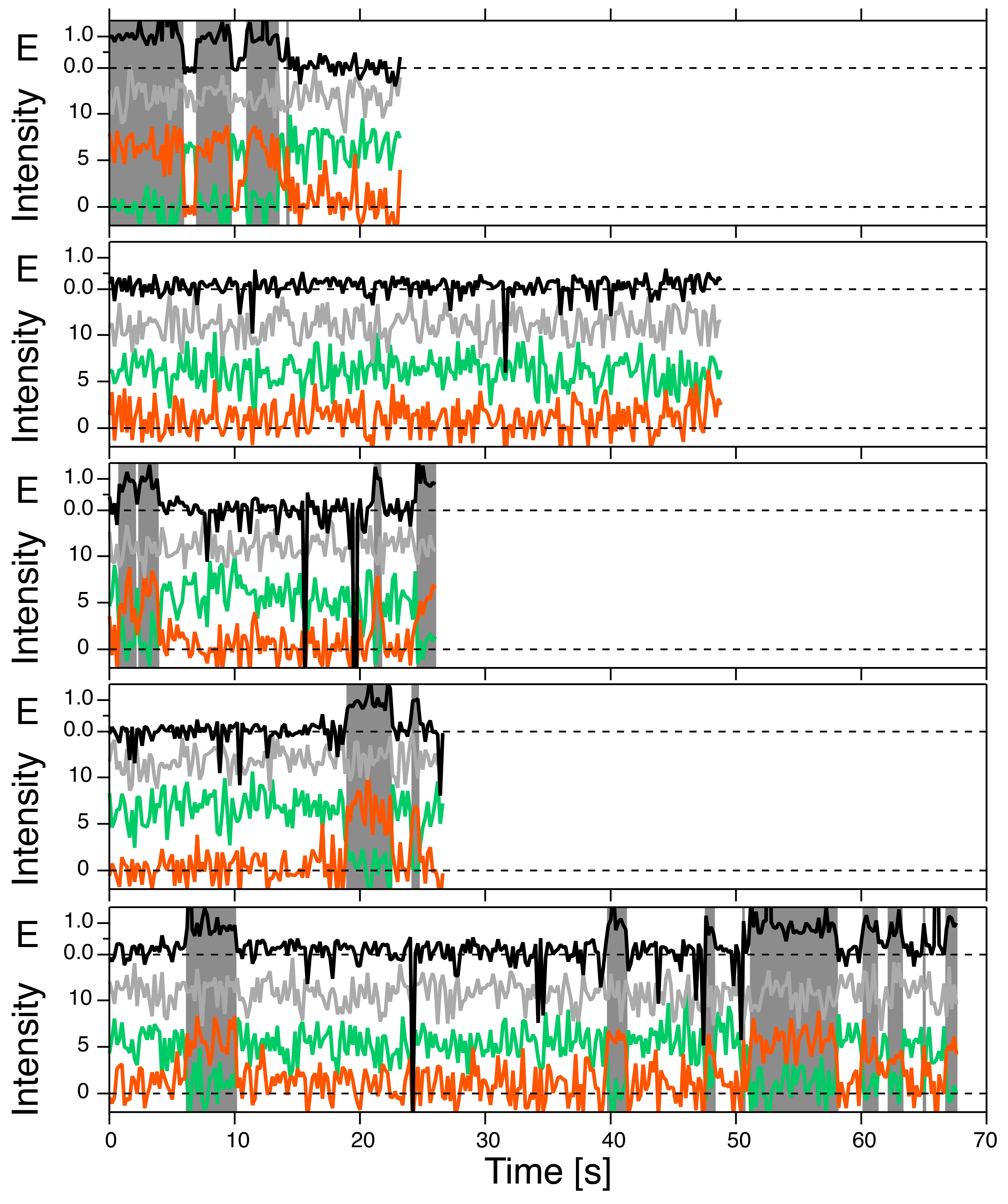
Figure 1: FRET efficiency vs. dwell time plots for a Holliday junction or Hsp90 (163 molecules) as indicated. Low FRET dwells in red; high FRET dwells in blue. No correlation is visible in either plot. In contrast to the Holliday junction, Hsp90’s conformational changes occur over a much broader time range.

Figure 2: Representative synthetic data generated by a 4-state model with 2x2 degenerate FRET efficiencies as described in the Online Methods. Fluorescence intensity of the donor (green), acceptor (orange) and acceptor after direct excitation (gray). Calculated FRET efficiency (E) in black and Viterbi path as overlays (two states: high FRET gray, low FRET white). Static traces (second trace) occur as a consequence of fast and slow rates together with a finite observation time due to photo-bleaching. FRET efficiency spikes occur in the simulations as well as in the experiment. In contrast to 1D HMM based on FRET, they have no effect on fluorescence based 2D HMM as can be seen from the Viterbi paths.

Figure 3: SMACKS as a flow chart.