System Aliasing in Dynamic Network Reconstruction:
Issues on Low Sampling Frequencies

Abstract

Network reconstruction of dynamical continuous-time (CT) systems is motivated by applications in many fields. Due to experimental limitations, especially in biology, data could be sampled at low frequencies, leading to significant challenges in network inference. We introduce the concept of “system aliasing” and characterize the minimal sampling frequency that allows reconstruction of CT systems from low sampled data. A test criterion is also proposed to check whether system aliasing is presented. With no system aliasing, the paper provides an algorithm to reconstruct dynamic network from data in the presence of noise. In addition, when there is system aliasing we perform studies that add additional prior information of the system such as sparsity. This paper opens new directions in modelling of network systems where samples have significant costs. Such tools are essential to process the available data in applications subject to current experimental limitations.

I Introduction

Many complex systems can be modeled as networks in applications to reveal and illustrate interactions between measured variables. A common characteristic of such networks is sparsity, where each variable in only involved in a few interactions. Such sparse networks are often presented in systems in nature. An example of the latter is the interaction between species such as genes and proteins in human cells; such interactions can be modeled by stochastic/ordinary differential equations, e.g. [1]. Such network models in biology help to understand, for instance, metabolic pathways, interactions between DNAs/proteins, and furthermore contribute to pathology of disease detection on or even clinical treatment to complicate diseases, e.g. [2]. Motivated by practical applications, reconstruction of sparse (Boolean) networks turns to be critical as more techniques have been available to acquire time-series data.

There has recently been quite some interest in the study of dynamic networks from different perspectives: network identifiability[3, 4], network module identifiability[5], network inference using discrete-time approaches[6, 7], etc. With regard to network inference, the factor that distinguishes itself from traditional system identification[8] is the particular request on sparse structures. To enhance sparsity, there are multiple methods are available: LASSO[9], iterative reweighted $l_{1}$/$l_{2}$ algorithms[10, 11], Sparse Bayesian Learning[12, 13], etc.

It deserves to be emphasized that the discrete-time approach for network inference is valid only if the sampling frequency is high enough, where the discrete-time model shares the same network structure as the continuous one that is the physical process (here we assume the dynamical systems evolve in continuous time in nature). To use discrete-time methods, one practical rule to choose sampling frequencies is taking ten times the bandwidth of the underlying, in this case assumed to be linear, systems[8]. However, in biological systems, most time-series data are sampled considerably slower than this empirical frequency, e.g. “high time-resolution” time series in [14], which usually cannot be solved by increasing sampling rates due to various constraints in biological experiments.

There have been several studies on the identification of continuous-time systems, e.g. [15, 16]. However, most methods request a high sampling frequency to guarantee certain simplifications on theoretical deductions or numerical calculations. Choosing a fairly low sampling frequency may trigger the problem of “system aliasing”, that is, multiple continuous-time systems produce exactly the same output samples, while having different network structures. To determine physical interconnections, it is inevitable to resorting to the identification of continuous-time models. With decrease of sampling frequencies, it becomes particularly challenging, nearly intractable, in theory and computation to identify sparse structures of continuous-time models.

In this paper, we first reveal the challenges due to the low sampling frequency by examples in Section III and then present a definition of system aliasing. A Nyquist-Shannon-like sampling theorem is presented in Section IV to determine the minimal sampling frequency that avoids the effect of system aliasing. Section V presents an algorithm to reconstruct sparse networks in the case of no system aliasing using low-sampling-frequency data. The case with system aliases is discussed in Section VI, which discusses the feasibility of exploring the ground truth in theory. The last section, Section VII, provides numerical examples to show performance of the proposed methods.

II Problem Formulation

Consider a filtered probability space $(\Omega,\mathcal{F},(\mathcal{F}_{t})_{t\in[0,\infty)},\mathbb{P})$, where the filtration is always assumed to be complete. Let $\{w(t):t\geq 0\}$ be the $n$-dimensional standard $\mathcal{F}_{t}$-Brownian motion. The physical plant/process in our study, as a dynamical system in continuous time, is modeled by the following stochastic differential equation

$$\mathrm{d}x=Ax\,\mathrm{d}t+Bu\,\mathrm{d}t+R\mathrm{d}w,$$ (1)

where $A\in\mathbb{R}^{n\times n}$ is stable, $R\in\mathbb{R}^{n\times n}$ is symmetric and positive definitive, the initial $x(t_{0})$ is a Gaussian random variable with mean $m_{0}$ and variance $R_{0}$, $t_{0}\geq 0$, and $w(t)$ is interpreted as disturbance on the state variables (or called process noise). The solution to (1) is an $\mathcal{F}_{t}$-adapted $n$-dimensional stochastic process $x(t)=(x_{1}(t),\cdots,x_{n}(t))_{t\geq t_{0}}$ such that

$$x(t)=x(t_{0})+\int_{t_{0}}^{t}\left(Ax(s)+Bu(s)\right)\,\mathrm{d}s+\int_{t_{0}}^{t}R\mathrm{d}w(s),$$

where $x(t_{0})\in\mathcal{F}_{t_{0}}$ and see [17] for the definition of stochastic integral. It is assumed that $x(t_{0}),w(t)$ are independent. The solution $x(t)$ is strong, that is, $x(t)$ is adapted to $\mathcal{F}_{t}^{w}\coloneqq\sigma(w_{u}\!:\!u\!\leq\!t)\vee\sigma(\mathcal{N})$ (i.e. the complete $\sigma$-field generated by $\{w_{u}\!:\!u\!\leq\!t\}$; see [17] for details). An input signal $\{u(t),t\geq t_{0}\}$ has been applied to the system, and the output $y$ of the system is observed at the discrete times $t_{0},t_{1},...,t_{N}$,

$$y(t_{k})=Cx(t_{k})$$ (2)

where $C=[I\;0]\in\mathbb{R}^{p\times p},\ p\!\leq\!n$, $t_{k}\triangleq t_{0}+kh$ and $h>0$ is the sampling period. Here the measurement noise is not included mainly due to that we have not yet given a definition of network models (see [3]) from state-space representations with measurement noises. The stochastic difference equation that relates the values of the state variable $x$ in (1) at the sampling instants[18, p. 82-85][19, chap. 2] is given by

$$x(t_{k+1})=A_{d}x(t_{k})+B_{d}u(t_{k})+v(t_{k}),$$ (3)

where

$$A_{d}=\exp({hA}),\quad B_{d}=\int_{0}^{h}\exp(sA)B\,\mathrm{d}s,$$ (4)

$\exp(\cdot)$ is the matrix exponential, and the Gaussian i.i.d. $v(t)$ has mean zero and covariance matrix

$$R_{d}=\int_{0}^{h}\exp({sA})R\exp({sA^{T}})\,\mathrm{d}s.$$ (5)

The linear dynamic network model of (1) is given as

$$y(t)=Q(q)y(t)+P(q)u(t)+H(q)e(t),$$ (6)

where $Q(q),P(q)$ and $H(q)$ are $p\times p$, $p\times m$ and $p\times p$ matrices of strictly-proper real-rational transfer functions respectively in terms of $q$, $q$ is the differential operator $qx(t)=\mathrm{d}x/\mathrm{d}t$, and $e(t)$ is the Gaussian white noise with zero mean and $\mathbb{E}[e(t)^{T}e(s)]=I\delta(t-s)$ (e.g. see [4]). The model (6) is called Dynamical Structure Function (DSF), firstly proposed in [3]. The network model defines path diagrams which show the interconnections between the elements of the output variable.

Definition 1 ([7]).

Let $\mathcal{G}=(V,E)$ be a digraph, where the vertex set $V=\{y_{1},\dots,y_{p},u_{1},\dots,u_{m}\}$ and the arc (directed edge) set $E$ is defined by

1. $(y_{j},y_{i})\in E\;\,\Leftrightarrow\;Q_{ij}(q)\neq 0$,

2. $(u_{k},y_{i})\in E\;\Leftrightarrow\;P_{ik}(q)\neq 0$,

3. $(y_{i},u_{k})\notin E,\;\forall i,k$.

Let $f$ be a map defined as

$$\begin{array}[]{rrll}f:&E&\rightarrow&S_{\text{TF}}\\ &(y_{j},y_{i})&\mapsto&Q_{ij}(q)\quad\mathrm{or}\quad(u_{k},y_{i})\mapsto P_{ik}(q),\end{array}$$

where $S_{\text{TF}}$ is a subset of single-input-single-output (SISO) (strictly) proper real rational transfer functions. We call the tuple $\mathcal{N}\coloneqq(\mathcal{G},f)$ a (linear) dynamic network, $f$ the (linear) dynamic capacity function of $\mathcal{N}$, and $\mathcal{G}$ the underlying digraph of $\mathcal{N}$, which is also called (linear) Boolean dynamic network.

This article focuses on the full-state measurement case, i.e. $C=I$, where $A$ in (1) coincides with $Q(q)$ in network models (6). Concerning the network identifiability[3], we assume $B$ to be diagonal (DSF, [3]) or particularly $B=I$ (the model used in [5]). Let the measurement be denoted by $Y^{N}\triangleq[y(t_{0}),\;y(t_{1}),\;\dots,\;y(t_{N})].$ We summarize the main problem in our study as follows:

Main Problem: Given the finite signal $Y^{N}$ in full-state measurement (i.e. $C=I$), with probably large $h$ (the sampling period) and small $N$ (the length of time series), infer the dynamic network $\mathcal{N}$ (or the Boolean $\mathcal{G}$), assuming that the ground truth $A$ is sparse and and $B$ is diagonal.

Remark 1.

The problem is challenging due to the following two major reasons:

• Since $h$ could be large, i.e. the sampling frequency is low, we have to estimate $A$ in order to determine $\mathcal{G}$ or $\mathcal{N}$ (see Figure 1).

• Since $N$ does not approach infinity, the estimation of $A_{d}$ from PEM (Prediction Error Minimization) or ML (Maximum Likelihood) may fail to identify $\mathcal{G}$ correctly by taking matrix logarithms, even though PEM/ML gives consistent estimation in theory.

Throughout the text, by default, we always deal with primary matrix functions, including $\exp$ (matrix exponential), $\log$ (matrix logarithm) and $\operatorname{Log}$ (the principal matrix logarithm in Theorem 4). Primary matrix functions refer to the ones defined via Jordan Canonical Form or equivalently via Polynomial Interpolation, Cauchy Integral Theorem [20, chap. 1]. The primary notion of matrix functions is of particular interest and the most useful in applications[20, 21].

III System Aliasing in Identification

III-A Observations on matrix logarithm

Supposing that ${A}_{d}$ has been perfectly estimated from samples, the estimate of the $A$ matrix for the continuous-time system is straightforwardly calculated by solving

$$\exp(h{A})={A}_{d}.$$ (7)

via matrix logarithm. However, referring to Theorem 18 [20], the equation (7) has several (in fact infititely many) solutions. Let us review the following observations on (7) to see the troubles from low sampling frequencies (i.e. $1/h$).

Observation 1: With the increase of $h$, the Boolean structures of $A$ (i.e. $\mathcal{G}$ determined from $A$) and $A_{d}-I$ become more and more different, as illustrated by Figure 1. The sampling frequency ($1/h$) deserves to be emphasized as a core factor in the categorization of different cases in our study:

• Case I: when $h$ is “very small” such that $A_{d}$ shares the same Boolean structure as $A+I$. Indeed, one can see it by $\exp(hA)=I+hA+\frac{h^{2}}{2!}A^{2}+\cdots$. Hence we can determine $\mathcal{G}$ by identifying discrete-time models;

• Case II: when $h$ is “large” but the ground truth $A$ is still the principle matrix logarithm of $A_{d}$;

• Case III: when $h$ is “even larger” such that the ground truth $A$ is no longer the principle logarithm of $A_{d}$.

The general network model (6) of Case I has been solved by discrete-time approaches , e.g. see [7, 6]. Case II is what we mainly studied in this paper. We call both Case I and II no system aliasing, as defined and studied in later sections.

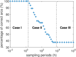
Figure 1: This example randomly chooses a sparse $A$ and $A_{d}=\exp(hA)$. The Boolean networks are determined from $A$ and $A_{d}-I$ by Definition 1 (treating $A$ and $A_{d}-I$ as $Q$’s), denoted by $\mathcal{G}(A),\mathcal{G}(A_{d}-I)$. We use $\mathcal{G}(A)$ as the ground truth. Then $\mathcal{G}(A_{d}-I)$ is compared with $\mathcal{G}(A)$ and the same arcs are labeled as the correct ones.

Observation 2: Provided with a sparse $A$, the corresponding $A_{d}$ could be dense, as the example in Figure 2.

Figure 2: $h=1$, $A_{d}=\exp{(hA)}$, $A=\operatorname{Log}{A_{d}}/h$.

Observation 3: Provided with a sparse $A$, the corresponding $A_{d}$ can be also sparse. However, they have different Boolean structures (i.e. zeros at different positions), as shown in Figure 3.

Figure 3: $h=1$, $A_{d}=\exp{(hA)}$, $A=\operatorname{Log}{A_{d}}/h$.

Observation 4: Even though the norm difference of $A_{d1},A_{d2}$ has been very small, their matrix logarithms, e.g. $A_{1}$ and $A_{2}$ in Figure 4, have significantly different Boolean structures.

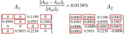
Figure 4: $h=1$, $A_{1}=\operatorname{Log}{A_{d1}}/h$ and $A_{2}=\operatorname{Log}{A_{d2}}/h$.

Observation 5: There exists more than one solution, e.g. $A_{1}$ and $A_{2}$ in Figure 5, and they have different Boolean structures.

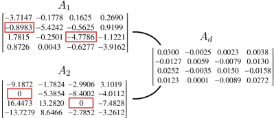
Figure 5: $h=1$, $\exp{(hA_{1})}=\exp{(hA_{2})}$, $A_{1}=\operatorname{Log}{A_{d}}/h$, and $A_{2}$ is the ground truth $A$.

Considering the problem formulation in Section II, one may have already noticed the troubles on network reconstruction, which originate from the matrix logarithms, due to the low sampling frequency. The examples in Observation 1 clearly show that why we have to resort to the continuous-time system identification to infer network structures. Observation 2 and 3 tell that there is no consistent relation between the sparsity of $A$ and $A_{d}$. Observation 4 points out that the Boolean structures of the principle logarithms of two $A_{d1}$ and $A_{d2}$ close in matrix norms could be significantly different. The example on Observation 5 shows an even worse case: the sample period is so large that the principle matrix logarithm is no longer $A$, which appears as other branches of matrix logarithm of $A_{d}$, in which no robust algorithm has yet been available.

Remark 2.

In a sum of the above observations, it tells us that, in the identification of $\mathcal{G}$ or $\mathcal{N}$,

• $\mathcal{G}$ should be determined from $A$ instead of $A_{d}$, when $h$ is large (w.r.t. $A$); (see Observation 1, 4)

• the sparsity penalty has to be imposed on $A$ directly instead of $A_{d}$, when $h$ is large (w.r.t. $A$); (see Observation 2, 3, 4)

• the $A$ matrix should be estimated directly instead of via taking matrix logarithm of $A_{d}$, in the presence of noise and a limited length of signals. (see Observation 4)

III-B Definitions

As shown in Section III-A, the $A$-matrix has to be identified in network reconstruction when the sampling frequency is low. In this scenario, a “good” case is that the ground truth $A$ stays as the principle matrix logarithm of $A_{d}$ (i.e. Case II); otherwise, it becomes particularly challenging (i.e. Case III), e.g. Figure 5. To clarify this classification, we consequently present an important concept in network reconstruction with low sampling frequencies, “system aliasing”.

Let $\operatorname{vec}(X)$ denote the vectorization of the matrix $X$ formed by stacking the columns of $X$ into a single column vector; and $\operatorname{ivec}(\cdot)$ is defined by $\operatorname{ivec}(\operatorname{vec}(X))=X$. $\operatorname{Im}(x)$ denotes the imaginary part of the complex number or vector $x$.

Definition 2.

$$\mathscr{E}(A,M,h,\mathscr{S})=\Big{\{}A^{*}\in\mathbb{R}^{n\times n}:\ M\in\mathbb{R}^{n^{2}\times n^{2}},h\in\mathbb{R},$$

$$A^{*}=\mathrm{arg}\min_{\tilde{A}\in\mathscr{S}}\|M\,\mathrm{vec}(\mathrm{exp}(hA))-M\,\mathrm{vec}(\mathrm{exp}(h\tilde{A}))\|_{2}\Big{\}},$$

where $\mathscr{S}\subseteq\mathbb{R}^{n\times n}$ contains $A$.

With this general notation, we present a definition of system aliasing only in terms of the $A$ matrix in state-space representations and the sampling period $h$, which does not depend on specific identification methods or data. Before presenting the concept of system aliasing, we have to assume no loss of information of input signals during sampling, e.g. no inputs, or the continuous input signal can be determined by input samples together with, for instance, the zero-order holder. Otherwise, we have to include constraints of input signals in our definition, which has not yet been studied.

Definition 3 (System aliasing).

Given $A\in\mathscr{S}$ and $h\in\mathbb{R}_{+}$, if there exists $\hat{A}\neq A\in\mathscr{E}(A,I,h,\mathscr{S})$ and $\hat{A}$ is called system alias of $A$ with respect to $\mathscr{S}$. By default, we choose $\mathscr{S}=\mathscr{S}_{A}\coloneqq\big{\{}\tilde{A}\in\mathbb{R}^{n\times n}:\max\{\operatorname{Im}(\operatorname{eig}(\tilde{A}))\}\leq\max\{\operatorname{Im}(\operatorname{eig}({A}))\}\big{\}}$.

We are particularly interested in $\mathscr{E}(A,I,h,\mathscr{S})=\{A\}$, i.e. there is no issue of system aliasing. Note that the concept of system aliasing does not depend on specific data. It only depends on system dynamics (e.g. the $A$-matrix in (1)) and sampling frequencies. If the $M$ matrix is specifically constructed by data instead of $I$, $\mathscr{E}(A,M,h,\mathscr{S})=\{A\}$, where $A$ denotes the ground truth, tells that the underlying system is identifiable from the given data (see [22, Sec. III-B]). Obviously if we have system aliasing for the system with a specific sampling frequency, without extra prior information on $A$, the system is always not identifiable.

IV No system aliasing: the minimal sampling frequency

Provided with the definition of system aliasing, a question comes first: what $(A,h)$ satisfies $\mathscr{E}(A,I,h,\mathscr{S}_{A})=\{A\}$. To answer this question, we need to introduce a theorem on matrix logarithm.

Theorem 4 (principal logarithm [20, Thm. 1.31]).

Let $P\in\mathbb{C}^{n\times n}$ have no eigenvalues on $\mathbb{R}^{-}$. There is a unique logarithm $A$ of P all of whose eigenvalues lie in the strip $\{z:-\pi<\operatorname{Im}(z)<\pi\}$. We refer to $A$ as the principal logarithm of $P$ of write $A=\operatorname{Log}(P)$. If $P$ is real then its principal logarithm is real.

To make the principal matrix logarithm $\operatorname{Log}(\cdot)$ be well-defined, we always assume that $\exp(hA)$ has no negative real eigenvalues. Let $\mathscr{G}(h)=\{z\in\mathbb{C}:-\pi/h<\operatorname{Im}(z)<\pi/h,h\in\mathbb{R}\}$. By Theorem 4 and 18, it always holds that $\operatorname{Log}(\exp(hA))/h\in\mathscr{E}(A,I,h,\mathscr{S}_{A})$. To avoid system aliasing, it implies that $\operatorname{Log}(\exp(hA))/h=A$ , i.e. $\operatorname{eig}(A)\in\mathscr{G}(h)$. It is summarized as the following lemma.

Lemma 5.

Let $A_{d}=\exp(hA),h\in\mathbb{R}_{+}$, which has no negative real eigenvalues, and $\hat{A}=\operatorname{Log}(A_{d})/h$. Then $A=\hat{A}$ (i.e. $\mathscr{E}(A,I,h,\mathscr{S}_{A})=\{A\}$) if and only if $\operatorname{eig}(A)\in\mathcal{G}(h)$.

Given no other information on the system, consider the identification problem of $A$ using full-state measurement. It is necessary to decrease the sampling period $h$ until the ground truth falls into the strip of $\mathscr{G}(h)$, and then the principal logarithm refers to the ground truth $A$, as illustrated in Figure 6. Otherwise, we would be bothered by system aliases of $A$ and be unable to make a decision, unless we know extra prior information on $A$.

Figure 6: The imaginary parts of all eigenvalues of $A$ must lie into $(-\pi/h,\pi/h)$. $\lambda_{i}(\cdot)$ denotes the $i$-th eigenvalue of $A$ in Theorem 18. The symbols “$\times$” denote the locations of $\operatorname{Im}(\lambda_{i}(A))$. $h_{\mathrm{max}}$ is the maximal sampling period that allows taking principal logarithms to estimate $A$, without facing troubles from system aliasing.

Theorem 6 (Nyquist-Shannon-like sampling theorem).

Considering equidistant sampling, to uniquely reconstruct the continuous-time system ${A}$ from the corresponding discrete-time system $A_{d}$ by taking the principal matrix logarithm, the sampling frequency $\omega$ (rad/s) must satisfy

$$\omega\geq 2\max\left\{|\operatorname{Im}\left(\lambda_{i}({A})\right)|,\ i=1,\dots,n\right\}.$$

Equivalently, the sampling period $h$ (i.e. $2\pi/\omega$) should satisfy

$$h\leq\min\left\{\pi/|\operatorname{Im}\left(\lambda_{i}({A})\right)|,\ i=1,\dots,n\right\}.$$

Proof.

The result immediately follows by verifying the condition $\operatorname{eig}(A)\in\mathcal{G}(h)$ in Lemma 5. ∎

Theorem 6 in continuous-time system identification can be understood by analogy with the Nyquist-Shannon sampling theorem in signal processing. The Nyquist-Shannon sampling theorem gives conditions on sampling frequencies, by looking at spectral information of signals, under which continuous signals can be uniquely reconstructed from their discrete-time signals. As an analogy, Theorem 6 addresses that continuous-time LTI systems can be uniquely reconstructed from their discrete-time systems under a condition that is built based on the spectral information of the $A$ matrix.

Now we would like to show a property of matrix exponential and logarithm, which further leads to a test criterion on system aliasing. See Appendix B for the proofs of Lemma 7 and Proposition 8.

Lemma 7.

Considering $h_{1},h_{2}\in\mathbb{R}_{+}$ and $A\in\mathbb{R}^{n\times n}$, let $\hat{A}$ be defined by $\hat{A}=\operatorname{Log}(\exp(h_{1}A))/h_{1}$. Then $\exp(h_{2}A)=\exp(h_{2}\hat{A})$ if and only if $h_{2}/h_{1}\in\mathbb{N}$ or $A=\hat{A}$.

Proposition 8.

Consider the dynamical system (1) without inputs (i.e. $B=0$), and two sampling periods $h_{1},h_{2}\in\mathbb{R}_{+}$ such that $h_{2}/h_{1}\notin\mathbb{N}$. Let $\hat{A}=\operatorname{Log}(\exp(h_{1}A))/h_{1}$ and $\hat{A}\neq A$. The one-step prediction errors w.r.t. $h_{2}$ are defined as

$$\epsilon(t_{k}) =x(t_{k})-\exp(h_{2}A)x(t_{k-1}),$$

$$\hat{\epsilon}(t_{k}) =x(t_{k})-\exp(h_{2}\hat{A})x(t_{k-1}).$$

Assuming that $\mathbb{E}(x(t_{k-1}))\neq 0$, it yields

$$\mathbb{E}(\epsilon(t_{k}))=0,\quad\mathbb{E}(\hat{\epsilon}(t_{k}))\neq 0.$$

We have similar results for the case with inputs, as stated in Proposition 22 in Appendix B, where we no longer require $\mathbb{E}(x(t_{k}))\neq 0$ due to the benefits from inputs. Meanwhile, according to the condition (39), it is possible that a carefully designed input signal invalidates the test criterion that is built by evaluating $\mathbb{E}(\hat{\epsilon}(t_{k}))$, which in practice may not be a problem. The results in Proposition 8 and Proposition 22 can be understood by Figure 7, where the output prediction of $\hat{A}$ (that is estimated from samples in $h_{1}$) presents different values from that of $A$ in another sampling period $h_{2}$ and it results in that the expectation of one-step prediction errors is no longer zero. The test criterion on system aliasing is summarized as follows:

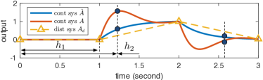
Figure 7: System responses of the dynamical system (1) with $A,\hat{A}$, where $A_{d}=\exp(h_{1}A),\hat{A}=\operatorname{Log}(A_{d})/h_{1}$, and the input signal is the square wave with period $2h_{1}$. The dots in deep blue are samples with the sampling period $h_{2}$.

Test Criterion (system aliasing).

Identify $A,B$ by PEM or ML (denoting the estimates by $\hat{A},\hat{B}$) assuming no system aliasing under the sampling period $h_{1}$, i.e. $\hat{A}$ asymptotically converges to $\operatorname{Log}(\exp(h_{1}A))$. Choose another sample period $h_{2}$ such that $h_{2}/h_{1}\notin\mathbb{N}_{+}$, and sample by $h_{2}$ the system responses with non-zero initial conditions or non-zero inputs (assuming (39) is satisfied). Use $\hat{A},\hat{B}$ to calculate the one-step prediction errors $\{\epsilon(t_{k})\}$. Perform t-test to obtain the p-value to make decisions, where the null hypothesis is that $\{\epsilon(t_{k})\}$ comes from a normal distribution with mean zero and unknown variance. Rejecting the null hypothesis implies the existence of system aliasing.

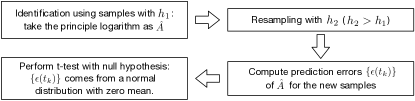
Figure 8: A chart flow of the test criterion on system aliasing.

V No system aliasing: sparse network reconstruction

Considering the systems given by  (1) and (2), the likelihood function is determined by the multiplication rule for conditional probability[23] $p(Y^{N}|\vartheta)\triangleq p(y(t_{N}),\dots,y(t_{1})|\vartheta)=p(y(t_{N})|y(t_{N-1}),\vartheta)\,p(y(t_{N-1})|y(t_{N-2}),\vartheta)\,\cdots p(y(t_{1})|\vartheta),$ where $\vartheta$ denotes the parameters under estimation, which parameterizes $A,B,R,m_{0},R_{0}$. With the assumption that $w(t),x(t_{0})$ are jointly Gaussian, the negative logarithmic likelihood function is

$$\begin{array}[]{@{}l@{\;}l@{\;}l}L(\vartheta)&=-2\log p(Y^{N}|\vartheta)=\sum_{k=1}^{N}\log\det\Lambda(t_{k},\vartheta)\\ &+\sum_{k=1}^{N}\epsilon^{T}(t_{k},\vartheta)\Lambda^{-1}(t_{k},\vartheta)\epsilon(t_{k},\vartheta)+\mathrm{const},\end{array}$$ (8)

where $\epsilon(t_{k},\vartheta)\coloneqq y(t_{k})-\hat{y}(t_{k}|t_{k-1},\vartheta)$, $\hat{y}(t_{k}|t_{k-1},\vartheta)$ denotes the conditional mean of $y(t_{k})$, and $\Lambda(t_{k},\vartheta)$ the corresponding covariance matrix. The optimal prediction of $y(t_{k})$ (i.e. $\hat{y}(t_{k}),\Lambda(t_{k})$) is obtained using Kalman filters (e.g. [23, 15]),

$$\begin{array}[]{r@{\;}l}\hat{y}(t_{k}|t_{k-1})&=C\hat{x}(t_{k}|t_{k-1})\\[1.42262pt] \hat{x}(t_{k}|t_{k})&=\hat{x}(t_{k}|t_{k-1})+K(t_{k})\epsilon(t_{k})\\ \displaystyle\frac{\mathrm{d}}{\mathrm{d}t}\hat{x}(t|t_{k})&=A\hat{x}(t|t_{k})+Bu(t),\quad t_{k}\leq t\leq t_{k+1}\\ K(t_{k})&=P(t_{k}|t_{k-1})C^{T}\Lambda^{-1}(t_{k})\\[1.42262pt] P(t_{k}|t_{k})&=P(t_{k}|t_{k-1})-K(t_{k})CP(t_{k}|t_{k-1})\\ \displaystyle\frac{\mathrm{d}}{\mathrm{d}t}P(t|t_{k})&=AP(t|t_{k})+P(t|t_{k})A^{T}+R,\quad t_{k}\leq t\leq t_{k+1}\\ \Lambda(t_{k})&=CP(t_{k}|t_{k-1})C^{T},\end{array}$$ (9)

where the initial condition is $\hat{x}(t_{1}|t_{0})=m_{0},\ P(t_{1}|t_{0})=R_{0}$. Considering the equidistant sampling and assuming the input is constant over the sampling periods, the matrix $\Lambda$ and $K$ appears in (9) can be treated as constant matrices by using steady-state Kalman filtering[23, Sec. 3.6].

Now consider the full-state measurement case (i.e. $C=I$) and restrict the noise to process noise. The calculation of prediction $\hat{y}(t_{k}|t_{k-1})$ becomes particularly simple since $K$ in (9) always equals the identity, which yields

$$\begin{array}[]{r@{\;}l}\epsilon(t_{k},\vartheta)&=y(t_{k})-A_{d}y(t_{k-1})-B_{d}u(t_{k-1}),\\ \Lambda(t_{k},\vartheta)&=R_{d},\end{array}$$ (10)

where $A_{d},B_{d},R_{d}$ are defined via $A,B,R$ in (4), (5). Here we resolve $p(y(t_{1})|\vartheta)$ by using $p(y(t_{1})|y(t_{0}),\vartheta)$, where $y(t_{0})$ is treated to be the deterministic and hence is removed from the conditional variables, and takes the first sample as its value. This simplification is due to the fact that $K\equiv I,P(t_{k}|t_{k})\equiv 0$ and the measurement of $x_{0}$ is available (using $y(t_{0})$), which also leads to that the best estimation of the distribution of $x_{0}$ is nothing better than a delta function (even if including the probability assumption of $x_{0}$ in maximum likelihood, i.e. $p(y(t_{1})|\vartheta)=p(y(t_{1})|y(t_{0}),\vartheta)p(y(t_{0})|\vartheta)$ and $p(y(t_{0})|\vartheta)$ takes the Gaussian density with mean $m_{0}$ and covariance matrix $R_{0}$). Alternatively, the likelihood function (8) can be obtained directly by considering (3) without using Kalman filtering. However, the above standard procedure values when we deal with general cases (i.e. $C\neq I$). Noticing the particular parameterization [8, p. 92, 206], maximizing likelihood can be performed as follows:

$$\hat{\theta} =\textstyle\operatorname{argmin}_{\theta}\sum_{k=1}^{N}\epsilon(t_{k},\theta)^{T}\epsilon(t_{k},\theta),$$ (11a)

$$\hat{R}_{d} =\textstyle\frac{1}{N}\sum_{k=1}^{N}\epsilon(t_{k},\hat{\theta})\epsilon^{T}(t_{k},\hat{\theta}),$$ (11b)

where $\theta$ is composed of $A,B$. To estimate $\theta$, instead of minimizing the prediction error as (11a), we impose the $l_{1}$-penalty to favor the sparse solution in network reconstruction. This is due to the observations in Section III-A: the consistency of ML may fail to present us with a correct network structure unless appropriate thresholds of zero for each row of $A,B$ are selected, which is hardly implemented in practice.

Remark 3.

If we include measurement noise or consider the output measurement case $C\neq I$, the prediction includes the Kalman filter gain $K$, which depends on $A,R$ and the covariance of measurement noise. It deserves to be emphasized that, due to the possible large sampling periods $h$, the numerical tricks used in [23, 15] may no longer be valid to compute the gradient of the prediction error. We have to analytically calculate the gradient as far as possible until the numerical computation is no longer restricted by $h$. This problem becomes fairly complicated.

V-A The cost function in matrix forms and the gradients

The reconstruction algorithm is supposed to infer a sparse network, i.e. $A$ is sparse. Due to the nonlinear least-square cost function (11a), it no longer satisfies the setup of Sparse Bayesian Learning proposed in [12]. Here we enhance sparsity by heuristically imposing the $l_{1}$-norm of $A$ as the penalty to the PEM cost function as the first tentative treatment.

Considering the measurement signal $Y^{N}$, let

$$\begin{array}[]{l@{\;}l}X_{+}&\triangleq[y(t_{1}),\;y(t_{2}),\;\dots,\;y(t_{N})],\\ X_{-}&\triangleq[y(t_{0}),\;y(t_{1}),\;\dots,\;y(t_{N-1})],\\ U_{-}&\triangleq[u(t_{0}),\;u(t_{1}),\;\dots,\;u(t_{N-1})],\end{array}$$

where $X_{+},X_{-}\in\mathbb{R}^{n\times N}$. The matrix form of the $l_{1}$-regularised PEM problem is formulated as

$$\begin{array}[]{l@{\;}l}\underset{A}{\operatorname{minimize}}&\big{\|}X_{+}-\exp(hA)X_{-}-\displaystyle\int_{0}^{h}\exp(sA)\,\mathrm{d}s\,BU_{-}\big{\|}_{F}^{2}\\ &+\lambda\left\|A\right\|_{1},\end{array}$$ (12)

where $\lambda\in\mathbb{R}^{+}$ and $h\in\mathbb{R}^{+}$ is the fixed and known sampling period, and the $l_{1}$ norm $\|A\|_{1}\coloneqq\sum_{i,j=1}^{n}|A_{ij}|$ ($A_{ij}$ denotes the $(i,j)$-th element of $A$). To avoid dealing with tensors, we use the vectorized form of (12) as follows:

$$\begin{array}[]{l@{\;}l}\underset{A}{\operatorname{minimize}}&\big{\|}\operatorname{vec}(X_{+})-(X_{-}^{T}\otimes I_{n})\operatorname{vec}(\exp(hA))\\ &-(U_{-}^{T}B^{T}\otimes I_{n})\displaystyle\int_{0}^{h}\operatorname{vec}(\exp(sA))\,\mathrm{d}s\big{\|}_{2}^{2}\\ &+\lambda\left\|\operatorname{vec}(A)\right\|_{1},\end{array}$$ (13)

where $\operatorname{vec}(X_{+})\in\mathbb{R}^{nN}$, $\operatorname{vec}(\exp(Ah))\in\mathbb{R}^{n^{2}}$, $(X_{-}^{T}\otimes I_{n})\in\mathbb{R}^{nN\times n^{2}}$, and $\otimes$ is the Kronecker product.

The problem (12) is challenging in optimization by noticing that it is: non-convex due to matrix exponential; not globally Lipschitz; and non-differentiable. The intuitive idea here is to use the the Gauss-Newton framework, in which each iteration is to solve a constrained $l_{1}$-regularized linear least square problem. Let

$$\begin{array}[]{l@{\;}l}r(A,B)\triangleq&\operatorname{vec}(X_{+})-(X_{-}^{T}\otimes I_{n})\operatorname{vec}(\exp(hA))\\ &-(U_{-}^{T}B^{T}\otimes I_{n})\displaystyle\int_{0}^{h}\operatorname{vec}(\exp(sA))\,\mathrm{d}s,\end{array}$$ (14)

$\phi(A,B)\coloneqq r(A,B)^{T}r(A,B)$, and $f(A,B)\triangleq\phi(A,B)+\lambda\|\operatorname{vec}(A))\|_{1}$, which is the objective function of (13). Then $\min_{A}\phi(A,B)$ denotes the problem (13) without $l_{1}$-penalisation. The gradient of $\phi(A,B)$ w.r.t. $A$ is $\nabla_{A}\phi=2J_{A}^{T}(A,B)r(A,B),$ where

$$J_{A}=-h(X_{-}^{T}\otimes I_{n})K(hA)-(U_{-}^{T}B^{T}\otimes I_{n})\displaystyle\int_{0}^{h}sK(sA)\,\mathrm{d}s,$$ (15)

and $K(A)$ is defined in Theorem 21. The function $sK(sA),s\!\in\![0,h]$ is integrable by noticing $\|sK(sA)\|\leq h\exp(h\|A\|)$ ($\|\cdot\|$ denotes any matrix norm). The matrix function $K(hA)$ and the integration can be calculated numerically given $A$. To compute the gradient of $\phi(A,B)$ w.r.t. $B$, using the matrix identity $\operatorname{vec}(AXB)=(B^{T}\otimes A)\operatorname{vec}(X)$ again for the term of $U$ in (12), it yields $\big{(}U_{-}^{T}B^{T}\otimes I_{n}\big{)}\int_{0}^{h}\operatorname{vec}(\exp(sA))\,\mathrm{d}s=\big{(}U_{-}^{T}\otimes\int_{0}^{h}\operatorname{vec}(\exp(sA))\,\mathrm{d}s\big{)}\operatorname{vec}(B).$ Then it follows that $\nabla_{B}\phi=2J_{B}^{T}(A,B)r(A,B),$ where

$$J_{B}=U_{-}^{T}\otimes\displaystyle\int_{0}^{h}\operatorname{vec}(\exp(sA))\,\mathrm{d}s.$$ (16)

If we assume $B$ is diagonal and $\nabla_{B}\phi$ is calculated w.r.t. each diagonal element of $B$, then $\nabla_{B}\phi=2\big{(}(I\otimes\mathbf{1})J_{B}\big{)}^{T}r(A,B)$, where $I$ is an $n\!\times\!n$ identity matrix and $\mathbf{1}$ is an $n^{2}$-dimensional row vector of 1’s. In a sum, the gradient of $\phi(A,B)$ is

$$\nabla\phi=\begin{bmatrix}\nabla_{A}\phi\\ \nabla_{B}\phi\end{bmatrix}=2\begin{bmatrix}J_{A}^{T}\\ J_{B}^{T}\end{bmatrix}r(A,B)\triangleq 2J^{T}(A,B)r(A,B).$$ (17)

V-B A special case: update A with fixed $B$

The subspace method in system identification presents us with nice initial estimation of $A_{0},B_{0}$ (e.g. see [24]). Concerning the task of network reconstruction, we would like to infer a sparse $A$ from data. As a special case, we only update $A$ by solving (12) with $B$ fixed to be $B_{0}$. For simplicity, in this subsection, let $r(A,B_{0})\triangleq r(A),J_{A}(A,B_{0})\triangleq J(A),\phi(A,B_{0})\triangleq\phi(A)$ and $f(A,B_{0})\triangleq f(A)$.

A linear approximation of $r(A)$ in a neighbourhood of a given point $A_{c}$ is $r(A_{c})+J(A_{c})\operatorname{vec}(A-A_{c}).$ One may then use this approximation and formulate a $l_{1}$-regularized linear least squares problem

$$\underset{A}{\operatorname{minimize}}\;\|r(A_{c})+J(A_{c})\operatorname{vec}(A-A_{c})\|_{2}^{2}+\lambda\|\operatorname{vec}(A)\|_{1},$$ (18)

which can be solved to obtain an approximate solution to (13). Resolving it in an iterative way amounts to a Gauss-Newton method. However, $\operatorname{vec}(A-A_{c})$ is not necessary to be a descent direction of (13).

In the $k$-th iteration, to guarantee the step $p_{k}=\operatorname{vec}(A-A_{k})$ being a descent direction of (13), the search direction $p_{k}$ is instead computed from the following constrained optimization problem

$$(P_{1})\left\{\begin{array}[]{@{\,}l@{\;\;}l}\underset{p_{k}\in\mathbb{R}^{n^{2}}}{\operatorname{minimize}}&\|r(A_{k})+J(A_{k})p_{k}\|_{2}^{2}+\lambda\|\operatorname{vec}(A_{k})+p_{k}\|_{1},\\ \operatorname{subject\ to}&\sup_{g\in\partial f(A_{k})}g^{T}p_{k}\leq 0,\end{array}\right.$$

where $\partial f(A_{k})$ denotes the subdifferential of $f(A)$ at $A_{k}$, defined as

$$\partial f(A_{k})\coloneqq\{\nabla\phi(A_{k})+\lambda z:z\in J_{1}\times\cdots J_{n^{2}}\},$$ (19)

$$J_{i}\coloneqq\begin{cases}[-1,1]&\text{if }\operatorname{vec}(A_{k})_{i}=0\\ \{1\}&\text{if }\operatorname{vec}(A_{k})_{i}>0\\ \{-1\}&\text{if }\operatorname{vec}(A_{k})_{i}<0\end{cases},$$ (20)

in which $\operatorname{vec}(A_{k})_{i}$ denotes the $i$-th element of $\operatorname{vec}(A_{k})$. One may have noticed that the constraint in the problem $(P_{1})$ is the definition of descent direction for $f$ at $A_{k}$, except replacing $<0$ with $\leq-\epsilon$ to guarantee the existence of minimum. The problem $(P_{1})$ is a convex optimization problem by noticing that $\sup_{g\in\partial f(A_{k})}g^{T}p_{k}$ is a convex function, which is a pointwise supremum over an infinite set of a linear function [25, chap. 3]. To solve the problem $(P_{1})$, we need to explore the constraint and derive an equivalent form (see Appendix C for details), given as follows.

$$(P_{1}^{\prime})\left\{\begin{array}[]{@{\,}l@{\;\;}l}\underset{p_{k}\in\mathbb{R}^{n^{2}}}{\operatorname{minimize}}&\|r(A_{k})+J(A_{k})p_{k}\|_{2}^{2}+\lambda\|\operatorname{vec}(A_{k})+p_{k}\|_{1},\\ \operatorname{subject\ to}&\bar{g}(A_{k})^{T}p_{k}+\lambda\|W(A_{k})p_{k}\|_{1}\leq 0,\end{array}\right.$$

where

$$\begin{array}[]{l@{\;}l}\bar{g}(A_{k})&=\nabla\phi(A_{k})+\lambda\operatorname{sgn}(A_{k}),\\ W(A_{k})&=I-\operatorname{diag}(|\operatorname{sgn}(A_{k})|),\end{array}$$ (21)

the identify matrix $I$ is of a compatible dimension, $|\cdot|$ denotes the element-wise absolute value, $\operatorname{diag}(v)$ denotes the diagonal matrix built from vector $v$, and the $\operatorname{sgn}$ function for vectors and matrices is extended from the standard signum function for real numbers, defined as follows: when $x\in\mathbb{R}^{n}$, $\operatorname{sgn}(x)$ denotes a $n$-dimensional vector whose $i$-th element equals $\operatorname{sgn}(x_{i})$; and when $X\in\mathbb{R}^{m\times n}$, $\operatorname{sgn}(X)\coloneqq\operatorname{sgn}(\operatorname{vec}(X))$. Now the problem $(P^{\prime})$ can be easily modeled using CVX in MATLAB and solved by standard optimization solvers [26].

The iterate is updated via

$$\operatorname{vec}(A_{k+1})=\operatorname{vec}(A_{k})+s_{k}p_{k},$$ (22)

where the step length $s_{k}$ is determined by backtracking line search. Let $f^{\prime}(A_{k};p_{k})$ denote the directional derivative of $f$ at $A_{k}$ in the direction $p_{k}$, by subcalculus,

$$\begin{array}[]{l@{\;}l}f^{\prime}(A_{k};p_{k})&\coloneqq\sup_{g\in\partial f(A_{k})}g^{T}p_{k}\\[4.0pt] &=\bar{g}(A_{k})^{T}p_{k}+\lambda\|W(A_{k})p_{k}\|_{1}.\end{array}$$ (23)

Given $\alpha\in(0,0.5),\beta\in(0,1)$ and an initial value $s_{k}=1$, the line search is to perform $s_{k}\leftarrow\beta s_{k}$ until

$$f\big{(}A_{k}+\operatorname{ivec}(s_{k}p_{k})\big{)}\leq f(A_{k})+\alpha s_{k}f^{\prime}(A_{k};p_{k}).$$ (24)

The whole iterative method for (13) is summarized in Algorithm 1. One has to note that this algorithm may not guarantee that the iterate will converges to the stationary point. It is lucky that we have good initial values of $A_{0},B_{0}$ to start with that is provided by the subspace method in system identification. Solving (12) is to search a sparse $A$ in the neighborhood of $A_{0}$. Moreover, we have the following propositions to guarantee fair properties of this algorithm. See Appendix C for the proofs.

Proposition 9.

Let $\hat{f}(A_{k},p_{k})$ denote the objective function of $(P_{1})$ and $p_{k}^{*}$ be its optimal point. If $p_{k}^{*}\neq 0$ and $\sup_{g\in\partial f(A_{k})}g^{T}p_{k}^{*}=0$, then $0\in\partial f(A_{k})$.

Proposition 10.

Let $\hat{f}(A_{k},p_{k})$ and $p_{k}^{*}$ be defined in Proposition 9. If $p_{k}^{*}=0$ and $0\in\operatorname{argmin}_{p_{k}}\hat{f}(A_{k},p_{k})$, then $0\in\partial f(A_{k})$.

Proposition 9 guarantees that the step $p_{k}^{*}$ from solving $(P_{1})$ will always be a descent direction of (13) (i.e. $\sup_{g\in\partial f(A_{k})}g^{T}p_{k}^{*}<0$) until either it reaches the stationary point or $\{p_{k}^{*}\}$ converges to zero. When $\{p_{k}^{*}\}$ approaches to zero, there are two cases: one is Proposition 10 which guarantees that it reaches the stationary point; the other is described as follows:

$p_{k}^{*}=0$ is the unique optimal point of $(P_{1})$ and $0\notin\operatorname{argmin}_{p_{k}}\hat{f}(A_{k},p_{k})$.

Regarding the second case, indeed, if there exists other optimal point $p_{k}^{**}\neq 0$ of $(P_{1})$, we instead consider $p_{k}^{**}$ using Proposition 9. This is why we restrict $p_{k}^{*}=0$ to be the unique optimum of $(P_{1})$. In the second case, $\{p_{k}^{*}\}$ converges to zero and the objective value $f(A_{k})$ also converges. However, in theory, we fail to prove that the limit point of $\{A_{k}+\operatorname{ivec}(p_{k}^{*})\}$ is a stationary point. In the sense of applications, it has been fairly good since we are looking up a sparse solution in the neighborhood of a fairly good estimate.

Algorithm 1 Modified Gauss-Newton for $l_{1}$-regularized nonlinear least square problems

1:given $\epsilon>0$, tolerance $\delta>0$; $\alpha\in(0,0.5)$, $\beta\in(0,1)$

2:initialize $A_{0},B_{0}$ by the subspace method.

3:repeat

4:    Calculate $r(A_{k}),J(A_{k}),\nabla\phi(A_{k})$ using (14), (15).

5:    Calculate $\bar{g}(A_{k}),W(A_{k})$ using (21).

6:    Compute the search direction $p_{k}$ by solving problem $(P^{\prime})$.

7:    Compute the directional derivative $f^{\prime}(A_{k};p_{k})$ using (23).

8:    Determine the step size $s_{k}$ by backtracking line search (24).

9:    Update the iterate $A_{k}$ by (22).

10:until $\|A_{k}-A_{k+1}\|_{2}<\delta$

Remark 4.

The proposed method can be considered as a variant of the damped Gauss-Newton method. If the Jacobian matrix $J(A_{k})$ does not have full column rank, one could adopt the Levenberg-Marquardt method and solve

V-C General cases: update both $A$ and $B$

Considering the vectorized form (13), let $\theta$ denote the optimal variables, i.e. $\theta\triangleq[\operatorname{vec}(A)^{T}\;\operatorname{vec}(\operatorname{diag}(B))^{T}]^{T}$, where $\operatorname{diag}(B)$ denotes the diagonal elements of $B$. The other notations follow that $r(A,B)\triangleq r(\theta),J(A,B)\triangleq J(\theta),\phi(A,B)\triangleq\phi(\theta)$ and $f(A,B)\triangleq f(\theta)$. In the same way as Section V-B, the approximated $l_{1}$-regularized linear least square problem with constraints is written as

$$(P_{2})\left\{\begin{array}[]{@{\,}l@{\;\;}l}\underset{p_{k}\in\mathbb{R}^{2n^{2}}}{\operatorname{minimize}}&\|r(\theta_{k})+J(\theta_{k})p_{k}\|_{2}^{2}+\lambda\|\operatorname{vec}(A_{k})+\Lambda p_{k}\|_{1},\\ \operatorname{subject\ to}&\sup_{g\in\partial f(\theta_{k})}g^{T}p_{k}\leq 0,\end{array}\right.$$

where $\Lambda=[I\;\>0]$ is of dimension $n^{2}\!\times\!2n^{2}$, $\partial f(\theta_{k})$ denotes the subdifferential of $f(\theta)$ at $\theta_{k}$, defined as

$$\partial f(\theta_{k})\coloneqq\{\nabla\phi(\theta_{k})+\lambda\Lambda^{T}z:z\in J_{1}\times\cdots J_{n^{2}}\},$$

and $J_{i},i=1,\dots,n^{2}$ are defined in (20). Equivalently, we solve the following convex-constrained convex problem to update $A,B$ by $\theta_{k+1}=\theta_{k}+p_{k}$.

$$(P_{2}^{\prime})\left\{\begin{array}[]{@{\,}l@{\;\;}l}\underset{p_{k}\in\mathbb{R}^{2n^{2}}}{\operatorname{minimize}}&\|r(\theta_{k})+J(\theta_{k})p_{k}\|_{2}^{2}+\lambda\|\operatorname{vec}(A_{k})+\Lambda p_{k}\|_{1},\\ \operatorname{subject\ to}&\bar{g}^{T}p_{k}+\lambda\|W(A_{k})\Lambda p_{k}\|_{1}\leq 0,\end{array}\right.$$

where $\bar{g}\triangleq\nabla\phi(\theta)+\lambda\Lambda^{T}\operatorname{sgn}(A_{k})$ and $W(A_{k})=I-\operatorname{diag}(|\operatorname{sgn}(A_{k})|)$. The backtracking line search is equipped in the same way as Section V-B and the algorithm trivially follows by modifying Algorithm 1.

VI System aliasing and bounded constraints

In the previous section we hinted that the conditions for no system aliasing follow as a consequence of bounded eigenvalues. In this section we follow this path and study the problem in the presence of system aliases.

Consider the case of system aliasing, i.e. $h$ is NOT chosen small enough such that $\mathscr{E}(A,I,h,\mathscr{S}_{A})=\{A\}$. In order to find out $A$ among the aliases we need extra information, for instance, the properties of $A$ known a priori. Here we assume that the ground truth $A$ is the sparest solution in $\mathscr{E}(A,I,h,\mathscr{S}_{\kappa})$ and $\kappa\in\mathbb{R}$ as an upper bound that has been prescribed. The set $\mathscr{S}_{\kappa}$ will be defined after giving Definition 11. $A$ can be searched by the criterion

$$\underset{\hat{A}\in\mathscr{E}(A,I,h,\mathscr{S}_{\kappa})}{\operatorname{minimize}}\|\hat{A}\|_{0}.\vspace*{-1.5mm}$$ (25)

Here is a niche that is the calculation of $\mathscr{E}(A,I,h,\mathscr{S}_{\kappa})$ from data. By definition,

$$\mathscr{E}(A,I,h,\mathscr{S}_{\kappa})=\big{\{}\tilde{A}\in\mathscr{S}_{\kappa}:\exp(h\tilde{A})=A_{d}\big{\}},$$ (26)

where $A_{d}=\exp(hA)$. Even if we know $A_{d}$ has consistent estimation via PEM or ML, considering the observations in Section III-A, we know the workflow, that is estimating $A_{d}$ and then obtaining $\mathscr{E}$ by matrix logarithms, is not robust in the presence of noise. In this section, we focus on studying the possibility of searching $A$ in the set of system aliases $\mathscr{E}(A,I,h,\mathscr{S}(\kappa))$ using the prior information.

Definition 11 ($Z$-weighted norm).

Let $h_{Z}(A)=Z^{-1}AZ$, where $Z$ is the matrix defined in Theorem 19. Then the norm is defined as $\|h_{Z}(\cdot)\|_{F}=\|\cdot\|_{F}\circ h_{Z}$.

To formulate $\mathscr{S}_{\kappa}$, we introduce this special norm of ${A}$, which is equivalent to the Frobenius norm up to a change of coordinates. The matrix $Z$ is constant, which can be obtained by Jordan decomposition of $A_{d}$. One can observe that

$$\|h_{Z}(\hat{A})\|_{F}=\text{vec}(\hat{A})^{T}(Z^{T}\otimes Z^{-1})^{T}(Z^{T}\otimes Z^{-1})\text{vec}(\hat{A})$$

is a proper $(Z^{T}\otimes Z^{-1})^{T}(Z^{T}\otimes Z^{-1})$-weighted vector norm in terms of $\operatorname{vec}(\hat{A})$. Using $\|h_{Z}(\cdot)\|_{F}$ is on the one hand simplifying the analysis we conduct throughout this section, and on the other explicitly penalizes the imaginary part of the eigenvalues without “distorting” them through the transformation by $Z$.

Now we define $\mathscr{S}_{\kappa}$ using the norm $\|h_{Z}(\cdot)\|_{F}$. The basic idea is that one should exclude such $A$’s whose imaginary parts of eigenvalues are too large, which implies their system response will show wild fluctuation, as illustrated in Figure. 9.

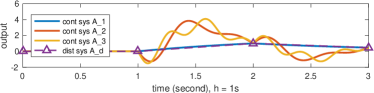
Figure 9: An example of system responses of multiple system aliases, i.e. $A_{i}\>(i\!=\!1,2,3)$ that satisfies $\exp(hA_{i})=A_{d}$, where $A_{2}$ is the ground truth but $A_{1}$ is the principle logarithm, and the input signal is a square wave of period $2h$.

That’s why we need to consider a reasonable set $\mathscr{S}_{\kappa}$ rather than $\mathbb{R}^{n\times n}$ in (26). In practice, even if we know the sampling frequency is not high enough to guarantee no system aliasing, we could still believe that the measurements do not miss too many fluctuation between samples. To make the constraint in (25) practically meaningful, we restrict $\mathscr{S}$ to be a norm bounded subset

$$\mathscr{S}_{\kappa}=\big{\{}\tilde{A}\in\mathbb{R}^{n\times n}:\|h_{Z}(\tilde{A})\|_{F}\leq\kappa\big{\}}.$$ (27)

In the following we will show that the feasible set of (25) has only finite elements, which implies it can be solved at least by brute force methods.

Let $M\coloneqq\operatorname{diag}(m_{1},m_{2},\dots,m_{p})$, $\textit{j}\coloneqq[j_{1},j_{2},\dots,j_{p}]$and $\beta\coloneqq[\beta_{1},\beta_{2},\dots,\beta_{p}]$, where $\log(\lambda_{k})\triangleq\alpha_{k}+i\pi\beta_{k}$, $k=1,\dots,p$, and $j_{k},\lambda_{k}$ are defined in Theorem 18. A function $\mathscr{I}$ is defined as

$$\mathscr{I}(\textit{j},\delta)\coloneqq\delta^{T}M\delta+(2\textit{j}+\beta)^{T}M\delta,$$ (28)

where $\textit{j},\delta\in\mathbb{Z}^{p}$. Moreover, it satisfies $\mathscr{I}(\textit{j},\delta)=\mathscr{I}(0,\textit{j}+\delta)-\mathscr{I}(0,\textit{j})$, which follows by noticing

$$\mathscr{I}(\textit{j},\delta)=\left(\delta+\textit{j}+{\beta}/{2}\right)^{T} M\left(\delta+\textit{j}+{\beta}/{2}\right)$$

$$-\left(\textit{j}+{\beta}/{2}\right)^{T} M\left(\textit{j}+{\beta}/{2}\right).$$ (29)

Moreover, let $A_{0}$ denote a special matrix logarithm for which all $j_{k}\ (k=1,\dots,p)$ in (33) are equal to $0$.

Definition 12 (equivalence relations).

Let $\mathcal{S}$ denote the set of all primary matrix logarithms

$$\mathcal{S}\coloneqq\big{\{}\tilde{A}\in\mathbb{R}^{n\times n}:\exp(h\tilde{A})=A_{d}\big{\}}.$$ (30)

An equivalence relation “$\sim$” is defined on $\mathcal{S}$ as a binary relation: for any $A_{1},A_{2}\in{\mathcal{S}}$, $\textit{j}^{(1)}$ and $\textit{j}^{(2)}$ are defined for $A_{1},A_{2}$, respectively, we say $A_{1}\sim A_{2}$ if $\mathscr{I}(\textit{j}^{(1)},\textit{j}^{(2)}-\textit{j}^{(1)})=0.$

Lemma 13.

Let ${\mathcal{S}}$ be the set defined in (26) and parametrized by (34) in Theorem 19. For any $A_{1},A_{2}\in{\mathcal{S}}$, $\|h_{Z}(A_{1})\|_{F}=\|h_{Z}(A_{2})\|_{F}$ if and only if $A_{1}\sim A_{2}$.

Lemma 14.

Given any $\bar{A}\in{\mathcal{S}}$, there exists a finite number of $A_{i}\in{\mathcal{S}}$ that satisfies $A_{i}\sim\bar{A}$.

Lemma 15.

There exists a finite number of $A_{i}\in{\mathcal{S}}$ such that $\|h_{Z}(A_{i})\|_{F}\leq\kappa$.

Proposition 16 (lower boundness of logarithms).

Let ${\mathcal{S}}$ be the set defined in (26). Given any $\bar{A}\in{\mathcal{S}}$, there exists $M(\bar{A})>0$, such that for any $A\in\{A\in{\mathcal{S}}:A\nsim\bar{A}\}$, it holds that

$$\left|\|h_{Z}(A)\|_{F}-\|h_{Z}(\bar{A})\|_{F}\right|\geq M.$$

Proposition 17.

Let ${\mathcal{S}}$ be the set defined in (26). For any $\bar{A}\in{\mathcal{S}}$, there exist $\kappa_{l},\kappa_{u}\in\mathbb{R}$ in $\mathscr{S}(\kappa_{l},\kappa_{u})=\{\tilde{A}\in\mathbb{R}^{n\times n}:\kappa_{l}\leq\|h_{Z}(\tilde{A})\|_{F}\leq\kappa_{u}\}$ such that (25) has a unique optimal point in the sense of the equivalence relation in Definition 12.

Proof.

It immediately follows by choosing

$$\kappa_{l} >\max\{0,\|h_{Z}(\bar{A})\|_{F}-M(\bar{A})\},$$

$$\kappa_{u} <\|h_{Z}(\bar{A})\|_{F}+M(\bar{A}),$$

where $M(\bar{A})$ is the lower bound on the gap between $\bar{A}$ and any $A\nsim\bar{A}\in{\mathcal{S}}$, defined in Theorem 16. ∎

VII Numerical examples

This section shows numerical examples of the proposed algorithm applied to 50 randomly generated datasets. The $A$ matrices in state space models are chosen to be random stable sparse matrices. Data is sampled from the simulation of stochastic differential equations, with $1/h$ set to be close to but larger than the critical sampling frequency by Theorem 6. The initial values of states were randomly sampled from Gaussian distributions with zero mean, and the process noise is Gaussian i.i.d, with SNR = 0 dB. Here, slightly abusing the name of “signals”, this “SNR” value is defined as $\text{SNR}=10\log(\sigma_{\text{init}}^{2}/\sigma_{\text{noise}}^{2})$, where $\sigma_{\text{init}}^{2}$ denotes the variance of random initial states and $\sigma_{\text{noise}}^{2}$ the variance of noise. Strictly speaking, $\text{SNR}=-\infty\,\text{dB}$ since the initial state is unknown in identification, and thus may not be treated as signals. We choose low sampling frequencies, large noise and limited samples to generate time series challenging in identification, however, which is a typical profile of time series in biological applications (e.g. microarray data [14]).

The random generation of sparse stable $A$ matrices is not a trivial task. Due to the lack of standards, it deserves time to explain our strategy to generate random $A$ matrices. First, we do not want the network to be separable (i.e. a collection of separate small networks). Thus, we first generate a loop of 24 nodes, which is represented by a stable $A$ matrix with nonzero diagonal and up-right (or bottom-left) corner elements. It serves as a base to build up $A$. Next a sparse matrix of the same dimension is generated with a fixed sparsity density. The $A$ matrix is finally obtained by overlapping the sparse matrix and the base and then permuting rows and columns randomly. During the operation of overlapping two matrices, it might be possible that the combined matrix is no longer stable. Therefore, we need a test of stability before releasing $A$ matrices. If the matrix turns into unstable, we simply discard it and search the next.

An example of time series is given in Figure 10.

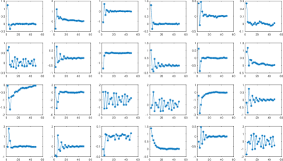
Figure 10: An example of time series used for reconstruction: 24 outputs, 24 samples, random initial states, no inputs, and SNR = 0 dB.

The reconstruction results of this dataset is shown in Figure 11, together with the corresponding $A_{d}$’s computed via matrix exponential. The straightforward way to estimate $A$ is taking the principal matrix logarithm of PEM/ML solution $\hat{A}_{d}$, which is, however, contaminated by process noise and unable to give reasonable sparse structure of $A$, clearly shown as $\hat{A}_{\mathrm{logm}}$in Figure 11(a). Taking matrix logarithm of least square estimations of $A_{d}$ mostly encounters the issue of non-existence of principle logarithms, which results in complex values of $A$. This shows the effects of process noise on then estimation through matrix logarithms. However, the direct logarithm of $\hat{A}_{d}$ might also work well when the dimension is small (e.g. $\mathrm{dim}(A)\leq 6$).

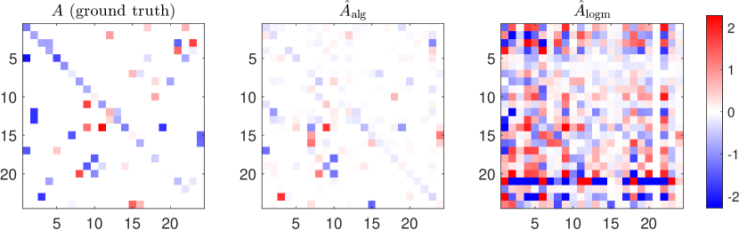
(a) Ground truth and the estimations of $A$

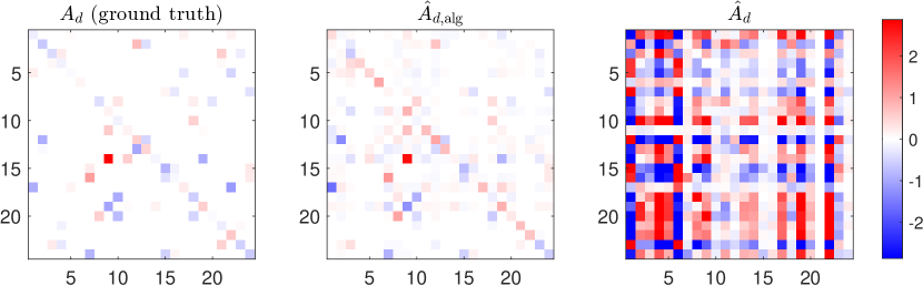
(b) Corresponding $A_{d}$ calculated by $\exp(hA)$

Figure 11: An example of network reconstruction results. $A$ and $A_{d}$ are the ground truth; $\hat{A}_{\mathrm{alg}}$ is estimated by the proposed method using $\lambda=0.01$, and $\hat{A}_{d,\mathrm{alg}}$ is calculated by $\exp(h\hat{A}_{\mathrm{alg}})$; $\hat{A}_{\mathrm{logm}}$ is the principal logarithm of $\hat{A}_{d}$ divided by $h$, and $\hat{A}_{d}$ is estimated by PEM or ML.

The curve of prediction errors is shown in Figure 12, which shows the convergence behaviors of Algorithm 1. Here the $\lambda$ is chosen by performing network reconstruction on one dataset using $\lambda$ logarithmically ranging from $10^{-4}$ to $100$ and checking the sparsity of $\hat{A}$’s (users’ prior knowledge) and the resultant prediction errors (whiteness, mean, standard deviations). This value of $\lambda$ is then applied to all the other datasets. Indeed, the choice of $\lambda$ also depends on $A$’s, which, however, is randomly generated with the same sparsity. That might explain why the same $\lambda$ works almost well for all datasets. Alternatively, $\lambda$ could be automatically calculated by running the cross-validation technique, when the amount of data allows. As widely used in bioinformatics, the Receiver Operating Characteristic (ROC) curve and the Precision-Recall (P-R) curve of this example are provided in Figure 13.

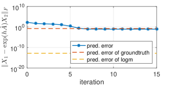
Figure 12: An example of convergence curve, with $\lambda=0.01$ and zero as the initial point, for the chosen data set in Figure 10.

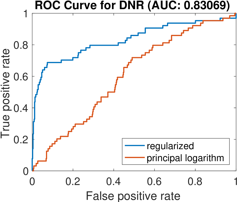
(a) ROC curve

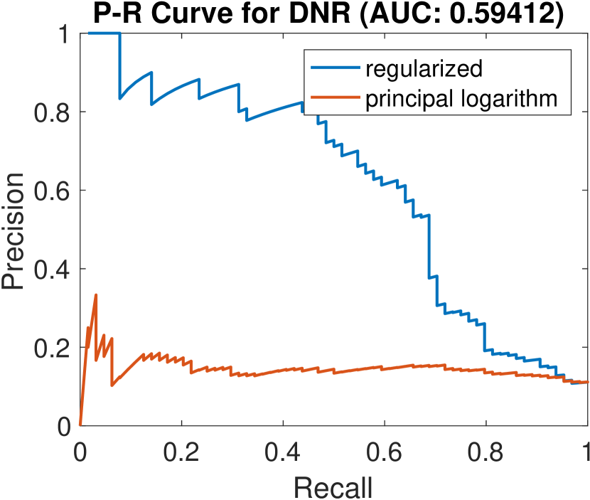
(b) P-R curve

Figure 13: The ROC and the Precision-Recall curves for the chosen example.

To show the performance of the proposed method, the ROC and the P-R curves, averaging over reconstruction results of 50 random systems, are shown in Figure 14. The variables used in ROC and P-R curves are computed by MATLAB function perfcurve with XVals fixed. However, one has to notice that, at certain values of “Recall” close to 0, the corresponding “Precision” is not defined, as shown in Figure 15(a), due to the fixed XVals. However, we need to fixed the value of XVals in order to take average of 50 P-R curves. One may notice the irregular profile of P-R curves for certain datasets, where the corresponding values of “Precision” drop to zero in the neighborhood of zero “Recall”.

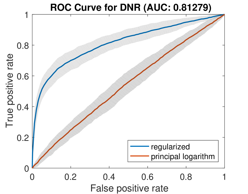
(a) ROC curve

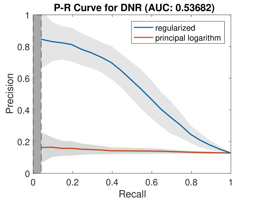
(b) P-R curve

Figure 14: The ROC and P-R curves averaging over the results of the proposed algorithm used on 50 random systems. The shaded area corresponds to one standard deviation from the mean value. The AUC values in titles refer to the mean of AUC values of the proposed method. The darkest area circled by dash lines is the uncertain region due to the average of NaN values in a few P-R curves.

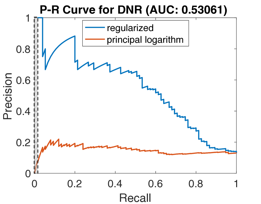
(a) regular P-R curve

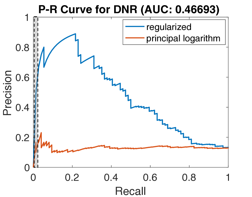
(b) irregular P-R curve

Figure 15: Examples of P-R curves which show regular shapes and irregular shapes, which is supplement to the explanation of undefined region in Figure 14(b). The shaded area in (a) is undefined region, which differs in different datasets; the one in (b) shows irregular profiles.

The numerical examples are programmed and computed in MATLAB, and the codes will be released in public on the github.com/oracleyue. Considering computational efficiency, we directly used vector/matrix norms instead of quadratic forms in implementation (cf. [26, chap. 11.1]). Thanks to the matrix function toolbox [27] and the CVX [28] for easy usage of matrix functions and convex optimisation in MATLAB.

VIII Conclusions

Continuous-time system identification is challenging when only low-sampling-frequency data with limited lengths are available. Unfortunately, this is a typical profile of time series in biomedicine applications. To reconstruct the correct dynamic networks from such time series, we have to identify the continuous-time models with sparse network structures. This paper studies the full-state measurement case, which is supposed to be the basic case while it shows particular complications. We first clarify the concept of system aliasing, which is raised by low sampling frequencies. A theorem on how to choose the sampling frequency to guarantee no system aliasing is provided, together with a test criterion. In regard to the “easy” case, i.e. no system aliasing, we present an algorithm to reconstruct sparse dynamic network from full-state measurements. In the case with system aliasing, the possibility on searching among system aliases is manifested in theory relying on the prior information on network sparsity. The paper dedicates to show the challenges and attract more people contributing to this study.

Appendix A Matrix Exponential and Logarithm

Theorem 18 (Gantmacher[20, Thm. 1.27]).

Let $P\in\mathbb{C}^{n\times n}$ be nonsingular with the Jordan canonical form

$$Z^{-1}PZ =J=\operatorname{diag}(J_{1},J_{2},...,J_{p})$$ (31a)

$$J_{k} =J_{k}(\lambda_{k})=\begin{bmatrix}\lambda_{k}&1&&\\ &\lambda_{k}&\ddots&\\ &&\ddots&1\\ &&&\lambda_{k}\end{bmatrix}\in\mathbb{C}^{m_{k}\times m_{k}}.$$ (31b)

Then all solutions to $e^{A}=P$ are given by

$$A=ZU\operatorname{diag}(L_{1}^{j_{1}},L_{2}^{j_{2}},...,L_{p}^{j_{p}})U^{-1}Z^{-1},$$ (32)

where

$$L_{k}^{j_{k}}=\log(J_{k}(\lambda_{k}))+2j_{k}\pi iI_{m_{k}};$$ (33)

$\log(J_{k}(\lambda_{k}))$ denotes

$$f(J_{k})\coloneqq\begin{bmatrix}f(\lambda_{k})&f^{\prime}(\lambda_{k})&\cdots&\frac{f^{(m_{k}-1)}(\lambda_{k})}{(m_{k}-1)!}\\ &f(\lambda_{k})&\ddots&\vdots\\ &&\ddots&f^{\prime}(\lambda_{k})\\ &&&f(\lambda_{k})\end{bmatrix}$$

with $f$ the principal branch of the logarithm, defined by $\mathrm{Im}(\log(z))\in(-\pi,\pi]$; $j_{k}$ is an arbitrary integer; and $U$ is an arbitrary nonsingular matrix that commutes with $J$.

Theorem 19 (classification of logarithms[20, Thm. 1.28]).

Let the nonsingular matrix $P\in\mathbb{C}^{n\times n}$ have the Jordan canonical form (31) with $p$ Jordan blocks, and let $s\leq p$ be the number of distinct eigenvalues of $A$. Then $e^{A}=P$ has a countable infinity of solutions that are primary functions of $P$, given by

$$A_{j}=Z\operatorname{diag}(L_{1}^{j_{1}},L_{2}^{(j_{2})},...,L_{p}^{(j_{p})})Z^{-1},$$ (34)

where $L_{k}^{j_{k}}$ is defined in (33), corresponding to all possible choices of the integers $j_{1},...,j_{p}$, subject to the constraint that $j_{i}=j_{k}$ whenever $\lambda_{i}=\lambda_{k}$.

If $s<p$ then $e^{A}=P$ has nonprimary solutions. They form parametrized families

$$A_{j}(U)=ZU\operatorname{diag}(L_{1}^{j_{1}},L_{2}^{(j_{2})},...,L_{p}^{(j_{p})})U^{-1}Z^{-1},$$ (35)

where $j_{k}$ is an arbitrary integer, $U$ is an arbitrary nonsingular matrix that commutes with $J$, and for each $j$ there exist $i$ and $k$, depending on $j$, such that $\lambda_{i}=\lambda_{k}$ while $j_{i}\neq j_{k}$.

Definition 20 (Fréchet Derivatives[20]).

The Fréchet derivative of the matrix function $f:\mathbb{C}^{n\times n}\rightarrow\mathbb{C}^{n\times n}$ at a point $X\in\mathbb{C}^{(n\times n)}$ is a linear mapping

$$\mathbb{C}^{n\times n} \overset{L}{\longrightarrow}\mathbb{C}^{n\times n}$$

$$E \longmapsto L(A,E)$$

such that for all $E\in\mathbb{C}^{n\times n}$

$$f(A+E)-f(A)-L(A,E)=o(\|E\|).$$

The Fréchet derivative is unique if it exists, and for matrix functions $\mathrm{exp}$ (matrix exponential) and $\mathrm{Log}$ (principal matrix logarithm) it exists. The Fréchet derivative of the function $\mathrm{exp}$ [20] is

$$L_{\mathrm{exp}}(X,E)=\int_{0}^{1}e^{X(1-s)}Ee^{Xs}ds,$$ (36)

which can be efficiently calculated by the Scaling-Pade-Squaring method in [29]. It gives a linear approximation of $\exp$ at a given point $A_{c}$ in the direction $E$

$$e^{hA}=e^{h({A}_{c}+E)}=e^{h{A}_{c}}+L(h{A}_{c},hE)+O(\|hE\|^{2}).$$ (37)

The Fréchet derivative of the function $\mathrm{Log}$ [20] is

$$L_{\mathrm{Log}}(X,E)=\int_{0}^{1}(t(X-I)+I)^{-1}E(t(X-I)+I)^{-1})dt,$$

and its efficient computation algorithm is provided in [30].

Theorem 21 (Kronecker representation [20, Thm. 10.13]).

For $A\in\mathbb{C}^{n\times n}$, $\operatorname{vec}(L(A,E))=K(A)\operatorname{vec}(E)$, where $K(A)\in\mathbb{C}^{n^{2}\times n^{2}}$ has the representations

$$(I\otimes e^{A})\psi\left(A^{T}\oplus(-A)\right)$$

$$(e^{A^{T}/2}\otimes e^{A/2})\operatorname{sinch}\left(\frac{1}{2}[A^{T}\oplus(-A)]\right)$$

$$\frac{1}{2}(e^{A^{T}}\oplus e^{A})\tau\left(\frac{1}{2}[e^{T}\oplus(-A)]\right)$$

where $\psi(x)=(e^{x}-1)/x$ and $\tau(x)=\tanh(x)/x$. The third expression is valid if $\frac{1}{2}\|A^{T}\oplus(-A)\|<\pi/2$ for some consistent matrix norm.

Here the operator $\oplus$ is the Kronecker sum, defined as

$$(A\oplus B)=A\otimes I_{n}+I_{m}\otimes B,$$

for $A\in\mathbb{R}^{m\times m}$ and $B\in\mathbb{R}^{n\times n}$.

Appendix B Test criteria on system aliasing

B-A A test criterion for the cases with inputs

Proposition 22.

Consider the dynamical system (1), and two sampling periods $h_{1},h_{2}\in\mathbb{R}_{+}$ such that $h_{2}/h_{1}\notin\mathbb{N}$. Let $f(A,B,h,t_{k})\triangleq x(t_{k})-\exp(hA)x(t_{k-1})-\int_{0}^{h}\exp(sA)B\,\mathrm{d}s\,u(t_{k-1})$, $\hat{A}=\operatorname{Log}(\exp(h_{1}A))/h_{1}$ and $\hat{B}$ be a value such that $\mathbb{E}(f(\hat{A},\hat{B},h_{1},t_{k})|x(t_{k-1}),u(t_{k-1}))=0$ for all $t_{k}$. The one-step prediction errors w.r.t. $h_{2}$ are defined as $\epsilon(t_{k})=f(A,B,h_{2},t_{k})$, $\hat{\epsilon}(t_{k})=f(\hat{A},\hat{B},h_{1},t_{k})$. If

$$\begin{array}[]{l@{}l}\mathbb{E}\Big{(}&\big{(}\exp(h_{2}A)-\exp(h_{2}\hat{A})\big{)}x(t_{k})\ +\\ &\displaystyle\int_{0}^{h_{2}}\big{(}\exp(sA)B-\exp(s\hat{A})\hat{B}\big{)}\mathrm{d}s\,u(t_{k})\Big{)}\neq 0,\end{array}$$ (39)

we have

$$\mathbb{E}(\epsilon(t_{k}))=0,\quad\mathbb{E}(\hat{\epsilon}(t_{k}))\neq 0.$$

The proof follows trivially by evaluating the expectation $\mathbb{E}(\hat{\epsilon}(t_{k}))$. We no longer require $\mathbb{E}(x(t_{k}))\neq 0$ since we can take advantages of $u(t_{k})$ to satisfy (39). In the cases with $\mathbb{E}(x(t_{k}))=0$ and non-zero inputs in expectation $\mathbb{E}(u(t_{k}))\neq 0$, assuming $A,\hat{A}$ are non-singular, the condition (39) can be further simplified as

$$\begin{array}[]{@{}l@{}l}&\big{(}\exp(h_{2}\hat{A})-I\big{)}\big{(}\exp(h_{1}\hat{A})-I\big{)}^{-1}\big{(}\exp(h_{1}{A})-I\big{)}\\ &\neq\exp(h_{2}A)-I.\end{array}$$ (40)

The simplification follows from (39) by noticing $\int_{0}^{h}e^{xs}\mathrm{d}s=(e^{hx}-1)/x$ and $A$ commutes with its matrix functions.

B-B Proof Lemma 7

Proof.

Let $A_{d}\coloneqq\exp(h_{1}A)$, which has the Jordan canonical form (31) (i.e. let $P$ in Theorem 18) be $A_{d}$). By Theorem 18 and 19, we have

$$\begin{array}[]{l@{\,}l@{\,}l@{}l}h_{1}A&=Z\operatorname{diag}(L_{1}^{j_{1}},&\dots,L_{p}^{j_{p}}&)Z^{-1},\\ h_{1}\hat{A}&=Z\operatorname{diag}(L_{1}^{0},&\dots,L_{p}^{0}&)Z^{-1}.\end{array}$$

To compare $\exp(h_{2}\hat{A})$ with $\exp(h_{2}A)$, we need to find their Jordan canonical form by the definition of matrix exponential. To calculate the eigenvalues of $h_{2}\hat{A}$, consider the determinant $|\hat{\mu}I-h_{2}\hat{A}|=0\Leftrightarrow|\hat{\mu}^{\prime}I-h_{1}\hat{A}|=0$, where $\hat{\mu}^{\prime}\triangleq h_{1}/h_{2}\hat{\mu}$ and $|\hat{\mu}^{\prime}I-h_{1}\hat{A}|=|\hat{\mu}^{\prime}I-\operatorname{diag}(L_{1}^{0},\dots,L_{p}^{0})|$. It is equivalent to solve $p$ equations $|\hat{\mu}_{k}^{\prime}I_{k}-L_{k}^{0}|=0\;(k=1,\dots,p)$, where $I_{k}$ denotes the identity matrix of the dimension compatible with $L_{k}^{0}$. It yields that

$$\begin{array}[]{l@{}l}&|\hat{\mu}_{k}^{\prime}I_{k}-L_{k}^{0}|=|\hat{\mu}_{k}^{\prime}I_{k}-\log(J_{k}(\lambda_{k}))|\\ &=\Big{|}\hat{\mu}_{k}^{\prime}I_{k}-\begin{bmatrix}\log(\lambda_{k})&\log^{\prime}(\lambda_{k})&\cdots&*\\ &\log(\lambda_{k})&\ddots&\vdots\\ &&\ddots&\log^{\prime}(\lambda_{k})\\ &&&\log(\lambda_{k})\end{bmatrix}\Big{|}\\ &=\left(\hat{\mu}_{k}^{\prime}-\log(\lambda_{k})\right)^{m_{k}}=0,\end{array}$$

where $J_{k},\lambda_{k},j_{k},m_{k},I_{m_{k}}$ are given in (31), (33); and hence $\mu_{k}=h_{2}/h_{1}\log(\lambda_{k})$ with geometric multiplicity $m_{k}$. Similarly for $h_{2}A$, consider $|\mu_{k}^{\prime}I_{k}-L_{k}^{j_{k}}|=|\mu_{k}^{\prime}I_{k}-\log(J_{k}(\lambda_{k}))-2j_{k}\pi iI_{m_{k}}|=0$, where $\mu_{k}^{\prime}\triangleq h_{1}/h_{2}\mu_{k}$, $\mu$ is the eigenvalues of $h_{2}A$, the integer $j_{k}$ is given in (33), and $i$ is the imaginary unit. It yields $m_{k}=h_{2}/h_{1}(\log(\lambda_{k})+2j_{k}\pi i)$ with multiplicity $m_{k}$. Considering the special forms of $L_{k}^{j_{k}}$, we have the following Jordan decomposition

$$\begin{array}[]{l@{\,}l}\operatorname{diag}(L_{1}^{0},\dots,L_{p}^{0})&=U\operatorname{diag}(J_{1}(\hat{\mu}_{1}),\dots,J_{p}(\hat{\mu}_{p}))U^{-1},\\[2.84526pt] \operatorname{diag}(L_{1}^{j_{1}},\dots,L_{p}^{j_{p}})&=U\operatorname{diag}(J_{1}({\mu}_{1}),\dots,J_{p}({\mu}_{p}))U^{-1},\end{array}$$

where $J_{k}(\hat{\mu}_{k})$ and $J_{k}(\mu_{k})$ denote the corresponding Jordan blocks. Therefore, $\exp(h_{2}A)=\exp(h_{2}\hat{A})$ is equivalent to $\exp(J_{k}(\mu_{k}))=\exp(J_{k}(\hat{\mu}_{k}))$ for any $k=1,\dots,p$, which implies $\exp(h_{2}/h_{1}2j_{k}\pi i)=0$. It leads to the conditions: $h_{2}/h_{1}\in\mathbb{N}_{+}$, or $j_{k}\equiv 0,\forall k$ (i.e. $\hat{A}=A$). ∎

B-C Proof of Proposition 8

Proof.

Considering the dynamical system (1), it is obvious that $\mathbb{E}(\epsilon(t_{k})|x(t_{k-1}))=0$. Now we evaluate the other expectation

$$\begin{array}[]{l@{\,}l}&\mathbb{E}\big{(}\hat{\epsilon}(t_{k})\big{)}=\mathbb{E}\big{(}x(t_{k+1})-\exp(h_{2}\hat{A})x(t_{k})\big{)}\\ &=\mathbb{E}\Big{(}\begin{array}[t]{@{}l@{}l}&\big{(}x(t_{k+1})-\exp(h_{2}A)x(t_{k})\big{)}+\\ &\big{(}\exp(h_{2}A)-\exp(h_{2}\hat{A})\big{)}x(t_{k})\Big{)}\end{array}\\ &=0+(\exp(h_{2}A)-\exp(h_{2}\hat{A}))\mathbb{E}(x(t_{k}))\neq 0,\end{array}$$

by Lemma 7. ∎

Appendix C More details on the optimization problems

C-A Equivalent forms of $(P_{1}),(P_{2})$

The following shows how to derive $(P_{1}^{\prime})$ from $(P_{1})$. Consider $g\in\partial f(A_{k})$ in $(P_{1})$, which implies $g=\nabla\phi(A_{k})+\lambda z=\nabla\phi(A_{k})+\lambda\operatorname{sgn}(A_{k})+\lambda(z-\operatorname{sgn}(A_{k}))\triangleq\bar{g}+\lambda(z-\operatorname{sgn}(A_{k}))$. Recall that $\max_{s\in[-1,1]^{n}}s^{T}x=\|x\|_{1}$ where $x$ is an $n$-dimensional vector. Then we have

$$\begin{array}[]{l@{\;}l}\displaystyle\sup_{g\in\partial f(A_{k})}g^{T}p_{k}&=\bar{g}^{T}p_{k}+\lambda\displaystyle\sup_{z\in J_{1}\times\cdots\times J_{n^{2}}}\left(z-\operatorname{sgn}(A_{k})\right)^{T}p_{k}\\ &=\bar{g}^{T}p_{k}+\lambda\displaystyle\sup_{\bar{z}\in[-1,1]^{l}}\bar{z}^{T}\left(W(A_{k})p_{k}\right)\\ &=\bar{g}^{T}p_{k}+\lambda\|W(A_{k})p_{k}\|_{1},\end{array}$$

where $W(A_{k})=I-\operatorname{diag}(|\operatorname{sgn}(A_{k})|)$ and $l=n^{2}-\operatorname{card}(\operatorname{sgn}(A_{k}))$.

Consider the optimization $(P_{2})$, we go through the same procedure and obtain

$$\sup_{g\in\partial f(\theta)}g^{T}p_{k}=\bar{g}^{T}p_{k}+\lambda\|W(A_{k})\Lambda p_{k}\|_{1},$$

where $\bar{g}\triangleq\nabla\phi(\theta)+\lambda\Lambda^{T}\operatorname{sgn}(A_{k})$.

C-B Proof of Proposition 9

Proof.

Without loss of generality, suppose that there exists $p^{*}_{k}\neq 0$ and $0\notin\operatorname{arg\,min}_{p_{k}}\hat{f}(A_{k},p_{k})$ such that $\sup_{g\in\partial f(A_{k})}g^{T}p^{*}_{k}=0$ and $0\notin\partial f(A_{k})$. (Indeed, if $0\in\operatorname{arg\,min}_{p_{k}}\hat{f}(A_{k},p_{k})$, we apply Proposition 10 and obtain $0\in\partial f(A_{k})$.) It implies that $\sup_{g\in\partial f(A_{k})}g^{T}\alpha p^{*}_{k}=0,\>\forall\alpha\in(0,1]$. Hence, $f(A_{k})\leq f(A_{k}+\alpha p_{k}^{*})$ for small enough $\alpha$. Let $\phi(A_{k}),\hat{\phi}(A_{k},p_{k})$ be defined by

$$\begin{array}[]{r@{\;}l}f(A_{k})&=\phi(A_{k})+\lambda\|\operatorname{vec}(A_{k})\|_{1},\\ \hat{f}(A_{k},p_{k})&=\hat{\phi}(A_{k},p_{k})+\lambda\|\operatorname{vec}(A_{k})+p_{k}\|_{1},\end{array}$$

and hence $\phi(A_{k}+\operatorname{ivec}(p_{k}))=\hat{\phi}(A_{k},p_{k})+o(\|p_{k}\|)$ ($\|\cdot\|$ denotes any vector norm). For simplicity, without any ambiguity, we use $f(A_{k}+p_{k})$ to represent $f(A_{k}+\operatorname{ivec}(p_{k}))$. Then we have $f(A_{k}+p_{k})=\hat{f}(A_{k},p_{k})+o(\|p_{k}\|)$, which yields

$$\lim_{\alpha\downarrow 0}\frac{|f(A_{k}+\alpha p_{k}^{*})-\hat{f}(A_{k},\alpha p_{k}^{*})|}{\alpha\|p_{k}^{*}\|}=0.$$ (41)

Now let us calculate this limit in a different way. Noting that $\hat{f}(A_{k},p_{k}^{*})\leq\hat{f}(A_{k},\alpha p_{k}^{*})$ (since $p_{k}^{*}\in\operatorname{arg\,min}_{p_{k}}\hat{f}(A_{k},p_{k})$) and $\hat{f}(A_{k},p_{k}^{*})<\hat{f}(A_{k},0)=f(A_{k})$ (since $0\notin\operatorname{arg\,min}_{p_{k}}\hat{f}(A_{k},p_{k})$), we have

$$\hat{f}(A_{k},\alpha p_{k}^{*})-f(A_{k})\geq\hat{f}(A_{k},p_{K}^{*})-f(A_{k})\geq\delta>0.$$

Moreover, since $f(A_{k}+\alpha p_{k}^{*})-f(A_{k})=\phi(A_{k}+\alpha p_{k}^{*})-\phi(A_{k})+\lambda(\|A_{k}+\alpha p_{k}^{*}\|_{1}-\|A_{k}\|_{1})=o(\alpha\|p_{k}^{*}\|)+O(\alpha\|p_{k}^{*}\|)$, there exists $M\in\mathbb{R}$ such that

$$\lim_{\alpha\downarrow 0}\frac{\left|f(A_{k}+\alpha p_{k}^{*})-f(A_{k})\right|}{\alpha\|p_{k}^{*}\|}\leq M.$$

Now we recalculate the limit in (41) as follows

$$\begin{array}[]{l@{\;}l}&\displaystyle\lim_{\alpha\downarrow 0}\frac{|f(A_{k}+\alpha p_{k}^{*})-\hat{f}(A_{k},\alpha p_{k}^{*})|}{\alpha\|p_{k}^{*}\|}\\ &\geq\displaystyle\lim_{\alpha\downarrow 0}\left|\frac{\left|f(A_{k}+\alpha p_{k}^{*})-f(A_{k})\right|}{\alpha\|p_{k}^{*}\|}-\frac{\left|f(A_{k})-\hat{f}(A_{k},\alpha p_{k}^{*})\right|}{\alpha\|p_{k}^{*}\|}\right|\\ &\geq\displaystyle\left|M-\lim_{\alpha\downarrow 0}\frac{\delta}{\alpha\|p_{k}^{*}\|}\right|=+\infty,\end{array}$$

which contradicts with (41). ∎

C-C Proof of Proposition 10

Proof.

Since $p_{k}^{*}\in\operatorname{argmin}_{p_{k}}\hat{f}(A_{k},p_{k})$, it yields $0\in\partial_{p}\hat{f}(A_{k},p_{k}^{*})$. Note that, in our discussion, $A_{k}$ is always fixed, and thus $\partial_{p}\hat{f}(A_{k},p_{k})$ denotes the subgradient of $\hat{f}(A_{k},\cdot)$ at $p_{k}$. Now let us write $\partial_{p}\hat{f}(A_{k},p_{k})$ explicitly

$$\partial_{p}\hat{f}(A_{k},p_{k})=\left\{\nabla\hat{\phi}(A_{k},p_{k})+\lambda\hat{z}:\hat{z}\in\hat{J}_{1}\times\cdots\hat{J}_{n^{2}}\right\},$$

where

$$\hat{J}_{i}=\begin{cases}[-1,1]&\text{if }\operatorname{vec}(A_{k})_{i}+(p_{k})_{i}=0\\ \{1\}&\text{if }\operatorname{vec}(A_{k})_{i}+(p_{k})_{i}>0\\ \{-1\}&\text{if }\operatorname{vec}(A_{k})_{i}+(p_{k})_{i}<0\end{cases},$$

$(p_{k})_{i}$ denotes the $i$-th element of $p_{k}$, and $\nabla\hat{\phi}(A_{k},p_{k})=2J(A_{k})^{T}\left(r(A_{k})+J(A_{k})p_{k}\right)$. Hence $\partial_{p}\hat{f}(A_{k},0)=\partial f(A_{k})$. Therefore, $0\in\partial_{p}\hat{f}(A_{k},p_{k}^{*})$ with $p_{k}^{*}=0$ implies $0\in\partial f(A_{k})$. ∎

Appendix D Proofs for boundness of system aliases

D-A Proof of Lemma 13

Proof.

Let $A_{i}\coloneqq Z\operatorname{diag}(L_{1}^{j_{1}^{(i)}},\cdots,L_{p}^{j_{p}^{(i)}})Z^{-1}$ , where $i=1,2$, $L_{k}^{j_{k}^{(i)}}\coloneqq\log(J_{k}(\lambda_{k}))+2j_{k}^{(i)}\pi iI_{m_{k}}$, and all other notations are given in (34).

$$\|h_{Z}({A}_{i})\|_{F}^{2}-\|h_{Z}({A_{0}})\|_{F}^{2} =\ \operatorname{tr}\left(\operatorname{diag}^{*}(L_{1}^{j_{1}^{(i)}},\cdots,L_{p}^{j_{p}^{(i)}})\operatorname{diag}(L_{1}^{j_{1}^{(i)}},\cdots,L_{p}^{j_{p}^{(i)}})\right)$$

$$\quad\ -\operatorname{tr}\left(\operatorname{diag}^{*}(L_{1}^{(0)},\cdots,L_{p}^{(0)})\operatorname{diag}(L_{1}^{(0)},\cdots,L_{p}^{(0)})\right)$$

$$=\textstyle\sum_{k=1}^{p}\operatorname{tr}\left(L_{k}^{j_{k}^{(i)}*}L_{k}^{j_{k}^{(i)}}-L_{k}^{(0)*}L_{k}^{(0)}\right)$$ (42)

$$=\textstyle\sum_{k=1}^{p}\operatorname{tr}\left(2j_{k}^{(i)}\pi i\left(\log(J_{k})^{*}-\log(J_{k})\right)+4\pi^{2}j_{k}^{(i)2}I_{m_{k}}\right)$$

$$=\textstyle\sum_{k=1}^{p}4\pi j_{k}^{(i)}m_{k}(\beta_{k}+j_{k}^{(i)})=4\pi\,\mathscr{I}(0,\textit{j}),\quad\textit{j}\triangleq[j_{1}^{(i)},\dots,j_{p}^{(i)}].$$

By using (42) for $A_{1},A_{2}$, we obtain

$$\|h_{Z}(A_{1})\|_{F}=\|h_{Z}(A_{2})\|_{F}\Leftrightarrow\|h_{Z}(A_{1})\|_{F}^{2}-\|h_{Z}(A_{0})\|_{F}^{2}$$

$$=\|h_{Z}(A_{2})\|_{F}^{2}-\|h_{Z}(A_{0})\|_{F}^{2}\Leftrightarrow\mathscr{I}(\textit{j}^{(1)},\textit{j}^{(2)}-\textit{j}^{(1)})=0,$$

which implies that $A_{1}\sim A_{2}$ by definition. The first equality in (42) is due to the linear transformation $h_{Z}(\hat{A})$. ∎

D-B Proof of Lemma 14

Proof.

Let j denote $[j_{1},\dots,j_{p}]$ of $\bar{A}$ in (33), and $\textit{j}^{(i)}$ denotes $[j_{1}^{(i)},\dots,j_{p}^{(i)}]$ of $A_{i}\in{\mathcal{S}}$. $\delta\triangleq\textit{j}^{(i)}-\textit{j}$, therefore $\delta\in\mathbb{Z}^{p}$, where $\succeq$ denote the element-wise larger-or-equal relation. By Definition 12, it is equivalent to show that $\mathscr{I}(\textit{j},\delta)=0$ has finite solutions, given j. We require $\delta$ to satisfy the following condition:

$$|\delta_{i}+j_{i}+\beta_{i}/2|\leq\sqrt{\frac{(\textit{j}+\beta/2)^{T}M(\textit{j}+\beta/2)}{m_{i}}}$$ (43)

for all $i=1,\dots,p$. Otherwise, supposing that there exists $i\in\{1,\dots,p\}$ such that $\delta_{i}$ does not satisfy (43), we will have

$$\mathscr{I}(\textit{j},\delta) =m_{i}(\delta_{i}+j_{i}+\beta_{i}/2)^{2}+\sum_{k\neq i}m_{k}(\delta_{k}+j_{k}\beta_{k}/2)^{2}$$

$$-\sum_{k}m_{k}(j_{k}+\beta_{k}/2)^{2}>\sum_{k\neq i}m_{k}(\delta_{k}+j_{k}\beta_{k}/2)^{2}\geq 0.$$

Let ${\mathcal{S}}^{\prime}\coloneqq\{A_{i}\in{\mathcal{S}}:j_{k}^{(i)}=\delta_{k}+j_{k},\delta_{k}\text{ satisfies \eqref{eq:delta-bound-eqiv-class}}\}$. We have $\{A_{i}\in{\mathcal{S}}:A_{i}\sim\bar{A}\}\subseteq{\mathcal{S}}^{\prime}$ and ${\mathcal{S}}^{\prime}$ is a finite set. ∎

D-C Proof of Lemma 15

Proof.

Let $\kappa_{0}\triangleq\|h_{Z}(A_{0})\|_{F}$. Then we need to show there exists a finite number of $A_{i}\in{\mathcal{S}}$ such that $\|h_{Z}(A_{i})\|_{F}^{2}-\|h_{Z}(A_{0})\|_{F}^{2}\leq\kappa^{2}-\kappa_{0}^{2}$, which is equivalent to show that there exists a finite number of solutions $\delta\in\mathbb{Z}$ to $\mathscr{I}(0,\delta)\leq(\kappa^{2}-\kappa_{0}^{2})/4\pi$. $\delta$ must satisfy the following condition:

$$|\delta_{i}+\beta_{i}/2|\leq\sqrt{\frac{(\beta/2)^{T}M(\beta/2)+(\kappa^{2}-\kappa_{0}^{2})}{m_{i}}}$$ (44)

for all $i=1,\dots,p$. Otherwise, by supposing that there exists $i\in{1,\dots,p}$ such that $\delta_{i}$ does not satisfy (44)leads to

$$\mathscr{I}(0,\delta) =m_{i}(\delta_{i}+\beta_{i}/2)^{2}+$$

$$\sum_{k\neq i}m_{k}(\delta_{k}+\beta_{k}/2)^{2}-(\beta/2)^{T}M(\beta/2)$$

$$> \sum_{k\neq i}m_{k}(\delta_{k}+\beta_{k}/2)^{2}+(\kappa^{2}-\kappa_{0}^{2})\geq\kappa^{2}-\kappa_{0}^{2}.$$

Note that the set of all $\delta\in\mathbb{Z}$ that satisfies (44) is finite, which finalizes the proof. ∎

D-D Proof of Proposition 16

Proof.

Let j denote $[j_{1},\dots,j_{p}]$ of $\bar{A}$ in (33), $N_{\mathrm{eqiv}}$ be the number of $A$’s that satisfy $A\sim\bar{A}$. Note that $|\|h_{Z}(A)\|_{F}^{2}-\|h_{Z}(\bar{A})\|_{F}^{2}|=|(\|h_{Z}(A)\|_{F}^{2}-\|h_{Z}(A_{0})\|_{F}^{2})-(\|h_{Z}(\bar{A})\|_{F}^{2}-\|h_{Z}(A_{0})\|_{F}^{2})|=|\mathscr{I}(\textit{j},\delta)|,\delta\in\mathbb{Z}$, which implies it is equivalent to show that $|\mathscr{I}(\textit{j},\delta)|,\delta\in\mathbb{Z}$ has a non-zero lower bound if not considering the $\delta$’s that result in $\mathscr{I}(\textit{j},\delta)=0$. We will prove it by contradiction. Assume this is not true, i.e. $\forall\epsilon>0$ there exists $\delta$ such that $0<|\mathscr{I}(\textit{j},\delta)|<\epsilon$. It implies that, arbitrarily given $\epsilon>0$, there exists an infinite number of $\delta$ such that $\mathscr{I}(\textit{j},\delta)<\epsilon$, which is impossible since $\mathscr{I}(0,\textit{j}+\delta)<\mathscr{I}(0,\textit{j})+\epsilon$ (using the fact that $\mathscr{I}(\textit{j},\delta)=\mathscr{I}(0,\textit{j}+\delta)-\mathscr{I}(0,\textit{j})$) has a finite number of solutions provided by Lemma 15. ∎

References

- [1] B. Ø. Palsson, Systems biology: simulation of dynamic network states. Cambridge University Press, 2011.
- [2] Z. Bar-Joseph, A. Gitter, and I. Simon, “Studying and modelling dynamic biological processes using time-series gene expression data,” Nature Reviews Genetics, vol. 13, no. 8, pp. 552–564, 2012.
- [3] J. Goncalves and S. Warnick, “Necessary and Sufficient Conditions for Dynamical Structure Reconstruction of LTI Networks,” Automatic Control, IEEE Transactions on, vol. 53, no. 7, pp. 1670–1674, 2008.
- [4] D. Hayden, Y. Yuan, and J. Goncalves, “Network Identifiability from Intrinsic Noise,” IEEE Transactions on Automatic Control, vol. PP, no. 99, p. 1, 2016.
- [5] P. M. J. Van den Hof, A. Dankers, P. S. C. Heuberger, and X. Bombois, “Identification of dynamic models in complex networks with prediction error methods-Basic methods for consistent module estimates,” Automatica, vol. 49, no. 10, pp. 2994–3006, 2013.
- [6] A. Chiuso and G. Pillonetto, “A Bayesian approach to sparse dynamic network identification,” Automatica, vol. 48, no. 8, pp. 1553–1565, 2012.
- [7] Z. Yue, W. Pan, J. Thunberg, L. Ljung, and J. Goncalves, “Linear Dynamic Network Reconstruction from Heterogeneous Datasets,” in Preprints of the 20th World Congress, IFAC, Toulouse, France, 2017, pp. 11 075–11 080.
- [8] L. Ljung, System Identification: Theory for the User, ser. Prentice-Hall information and system sciences series. Prentice Hall PTR, 1999.
- [9] M. Yuan and Y. Lin, “Model selection and estimation in regression with grouped variables,” Journal of the Royal Statistical Society: Series B (Statistical Methodology), vol. 68, no. 1, pp. 49–67, 2006.
- [10] E. J. Candes, M. B. Wakin, and S. P. Boyd, “Enhancing sparsity by reweighted l1 minimization,” Journal of Fourier analysis and applications, vol. 14, no. 5-6, pp. 877–905, 2008.
- [11] R. Chartrand and W. Yin, “Iteratively reweighted algorithms for compressive sensing,” in Acoustics, speech and signal processing, 2008. ICASSP 2008. IEEE international conference on. IEEE, 2008, pp. 3869–3872.
- [12] M. E. Tipping, “Sparse Bayesian learning and the relevance vector machine,” The journal of machine learning research, vol. 1, pp. 211–244, 2001.
- [13] D. P. Wipf and B. D. Rao, “An empirical Bayesian strategy for solving the simultaneous sparse approximation problem,” Signal Processing, IEEE Transactions on, vol. 55, no. 7, pp. 3704–3716, 2007.
- [14] F. He, H. Chen, M. Probst-Kepper, R. Geffers, S. Eifes, A. del Sol, K. Schughart, A. Zeng, and R. Balling, “PLAU inferred from a correlation network is critical for suppressor function of regulatory T cells,” Molecular Systems Biology, vol. 8, no. 1, nov 2012.
- [15] L. Ljung and A. Wills, “Issues in sampling and estimating continuous-time models with stochastic disturbances,” Automatica, vol. 46, no. 5, pp. 925–931, may 2010.
- [16] H. Garnier, M. Mensler, and A. Richard, “Continuous-time model identification from sampled data: implementation issues and performance evaluation,” International Journal of Control, vol. 76, no. 13, pp. 1337–1357, 2003.
- [17] J.-F. L. Gall, Brownian Motion, Martingales, and Stochastic Calculus (Graduate Texts in Mathematics), 1st ed. Springer, 2016.
- [18] K. J. Åström, Introduction to stochastic control theory. Courier Corporation, 2012.
- [19] H. Garnier and L. Wang, Identification of Continuous-time Models from Sampled Data. Springer London, 2008.
- [20] N. Higham, Functions of Matrices. Society for Industrial and Applied Mathematics, 2008.
- [21] R. A. Horn and G. G. Piepmeyer, “Two applications of the theory of primary matrix functions,” Linear Algebra and its Applications, vol. 361, pp. 99–106, mar 2003.
- [22] Z. Yue, J. Thunberg, and J. Goncalves, “Inverse Problems for Matrix Exponential in System Identification: System Aliasing,” in 2016 22nd Proceedings of International Symposium on Machematical Theory of Networks and Systems, 2016.
- [23] K. J. Åström, “Maximum likelihood and prediction error methods,” Automatica, vol. 16, no. 5, pp. 551–574, 1980.
- [24] M. Viberg, “Subspace-based state-space system identification,” Circuits, Systems and Signal Processing, vol. 21, no. 1, pp. 23–37, 2002.
- [25] S. Boyd and L. Vandenberghe, Convex optimization. Cambridge university press, 2004.
- [26] M. C. Grant and S. P. Boyd, The CVX Users’ Guide, Release v2.1, 2015. http://web.cvxr.com/cvx/doc/CVX.pdf
- [27] N. J. Higham, “The Matrix Function Toolbox: A MATLAB toolbox connected with functions of matrices.” jul 2008. http://www.mathworks.com/matlabcentral/fileexchange/20820-the-matrix-function-toolbox
- [28] I. CVX Research, “CVX: Matlab software for disciplined convex programming,” aug 2008. http://cvxr.com/cvx
- [29] A. H. Al-Mohy and N. J. Higham, “Computing the Fréchet derivative of the matrix exponential, with an application to condition number estimation,” SIAM Journal on Matrix Analysis and Applications, vol. 30, no. 4, pp. 1639–1657, 2009.
- [30] A. H. Al-Mohy, N. J. Higham, and S. D. Relton, “Computing the Fréchet derivative of the matrix logarithm and estimating the condition number,” SIAM Journal on Scientific Computing, vol. 35, no. 4, pp. C394–C410, 2013.