Simultaneous analysis of matter radii, transition probabilities, and excitation energies of Mg isotopes by angular-momentum-projected configuration-mixing calculations

Abstract

We perform simultaneous analysis of (1) matter radii, (2) $B(E2;0^{+}\rightarrow 2^{+})$ transition probabilities, and (3) excitation energies, $E(2^{+})$ and $E(4^{+})$, for ^24-40Mg by using the beyond mean-field (BMF) framework with angular-momentum-projected configuration mixing with respect to the axially symmetric $\beta_{2}$ deformation with infinitesimal cranking. The BMF calculations successfully reproduce all of the data for $r_{\rm m}$, $B(E2)$, and $E(2^{+})$ and $E(4^{+})$, indicating that it is quite useful for data analysis, particularly for low-lying states. We also discuss the absolute value of the deformation parameter $\beta_{2}$ deduced from measured values of $B(E2)$ and $r_{\rm m}$. This framework makes it possible to investigate the effects of $\beta_{2}$ deformation, the change in $\beta_{2}$ due to restoration of rotational symmetry, $\beta_{2}$ configuration mixing, and the inclusion of time-odd components by infinitesimal cranking. Under the assumption of axial deformation and parity conservation, we clarify which effect is important for each of the three measurements, and propose the kinds of BMF calculations that are practical for each of the three kinds of observables.

I Introduction

Recent measurements of reactions with radioactive beams have provided much information on unstable nuclei. Of particular interest is the island of inversion (IoI), where the neutron number $N$ is around 20 and the proton number $Z$ is from 10 (Ne) to 12 (Mg). In this region, the $N=20$ magic number does not give a spherical ground state, because a largely deformed shape is more favorable. In fact, it has very recently been reported as a result of measurements of total reaction cross sections $\sigma_{\rm R}$ Takechi-Mg ; Watanabe14 that the quadrupole deformation parameter $\beta_{2}$ jumps up to large values at $N=19$ for both Ne and Mg isotopes and maintains these large values up to at least the vicinity of the neutron drip line (i.e., up to $N=22$ for Ne isotopes and $N=26$ for Mg isotopes). Other experiments have also shown that the low-$N$ end of the IoI is $N=19$ Sorlin:2008jg . The low-$N$ end is thus rather well established, but the high-$N$ end is still under debate and hence the location is being intensively studied both experimentally and theoretically; see, for example, Refs. Hamamoto:2012mx ; Door13 ; Koba14 ; Caur14 .

Rich experimental data have already been accumulated for Mg isotopes in particular. In fact, data on $\sigma_{\rm R}$ are available for both even and odd $N$ up to $N=26$ Takechi-Mg ; Watanabe14 , data for $B(E2;0^{+}\rightarrow 2^{+})$ transition probabilities are available for even $N$ up to $N=22$ Moto95 ; Prit99 ; Chiste01 ; NNDC , and data for excitation energies $E(2^{+})$ and $E(4^{+})$ are available for even $N$ up to $N=26$ NNDC ; Door13 . Among these three kinds of observables, $B(E2)$ is the most useful for studying the $\beta_{2}$ deformation, but it is also the most difficult to measure as demonstrated by the limited amount of data. For this reason, $E(2^{+})$ and $E(4^{+})$ are often measured instead of $B(E2)$, particularly for nuclei near the neutron dripline. The ratio $E(4^{+})/E(2^{+})$ is a convenient quantity for seeing how close nuclei are to the ideal rotor or the vibration model.

The quadrupole deformation parameter $\beta_{2}$ is dimensionless and hence a convenient quantity for examining the $N$ and $Z$ dependence of nuclear deformation, and is often estimated from measured $B(E2;0^{+}\rightarrow 2^{+})$. However, this estimation requires that the root mean square (rms) matter radius $r_{\rm m}=\sqrt{\langle r^{2}\rangle}$ is properly obtained, c.f., Eqs. (4) and (17) below. In actual data analyses, the empirical formula $1.2A^{1/3}$ [fm] is widely used as a nuclear radius, where $A$ is the mass number. The corresponding rms radius is $r_{\rm m}^{\rm emp}=1.2A^{1/3}\sqrt{3/5}$ [fm], when a uniform density is assumed. However, it is necessary to confirm whether the empirical formula is reasonable. In unstable nuclei it is expected that $r_{\rm m}$ is larger than $r_{\rm m}^{\rm emp}$ because of the weakly bound nature, and hence it is possible that the expansion effect may be misinterpreted as an increase in $\beta_{2}$ deformation. It is therefore quite important to measure the matter radius $r_{\rm m}$.

The total reaction cross section $\sigma_{\rm R}$ is sensitive to the value of $r_{\rm m}$. In fact, the values of $r_{\rm m}$ have been deduced accurately for ^24-38Mg Watanabe14 by using the $g$-matrix folding model Minomo-DWS ; Minomo:2011bb ; Sumi:2012 from measured $\sigma_{\rm R}$ Takechi-Mg . The deduced data can be regarded as experimental data for $r_{\rm m}$ because of the accuracy of the model analyses. The $r_{\rm m}$ values thus obtained are plotted against $A$ in Fig. 1, where the finite-size effect of the nucleons is subtracted from the experimental data. The experimental values are larger than the results (dashed line) of the spherical Hartree–Fock–Bogoliubov (HFB) calculations with finite-range Gogny-D1S force DeGo80 ; D1S . The difference comes from the effect of deformations, predominantly of quadrupole type, as shown later in Sec. III.2. This is a good example of the fact that high-precision measurement of $\sigma_{\rm R}$ is useful for determining the actual value of $r_{\rm m}$ including the effect of deformations. The empirical rms radius $r_{\rm m}^{\rm emp}=1.2A^{1/3}\sqrt{3/5}$ [fm] is also plotted in Fig. 1 as a solid line. The difference between the dashed and solid lines is rather large, and we can thus conclude that the data for $B(E2)$ and $r_{\rm m}$ needs to be analyzed simultaneously in order to extract the $\beta_{2}$ deformation parameter.

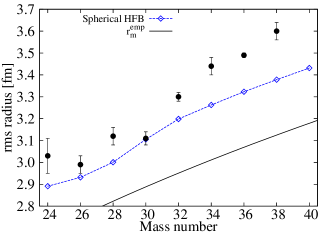
Figure 1: (Color online) $A$ dependence of matter radii for Mg isotopes. Dots with error bars show the experimental data deduced from the measured $\sigma_{\mathrm{R}}$, where the finite-size effect of the nucleons is subtracted from the experimental data. The dashed line indicates the results of spherical HFB calculations. The empirical rms radius $r_{\rm m}^{\rm emp}=1.2A^{1/3}\sqrt{3/5}$ [fm] is also plotted as a solid line.

Measurement of $\sigma_{\rm R}$ offers the advantage over $B(E2)$ and/or $E(2^{+})$ and $E(4^{+})$ that the measurement is relatively easy and possible for all combinations of even-even, even-odd, and odd-odd nuclei. In this paper, however, we concentrate our discussion on even-even Mg isotopes in order to analyze all the data for $r_{\rm m}$, $B(E2)$, and $E(2^{+})$ and $E(4^{+})$, simultaneously.

Taking ³²Mg with $N=20$ as a representative nucleus in the IoI, many mean-field calculations yield a spherical shape for the ground state (see, e.g., Refs.TFH97 ; LFS98 ; RDN99 ) because of the $N=20$ magicity. As mentioned above, however, large deformation has been reported for this nucleus by measurements of $B(E2;0^{+}\rightarrow 2^{+})$ Moto95 ; Prit99 ; Chiste01 , $E(2^{+})$ and $E(4^{+})/E(2^{+})$ NNDC , and $\sigma_{\rm R}$ Takechi-Mg , that is, $r_{\rm m}$ at $A=32$ in Fig. 1. In contrast, for ⁴⁰Mg with $N=28$, mean-field calculations predict a deformed ground state TFH97 ; LFS98 ; RDN99 . The shell closure is thus more fragile for $N=28$ than for $N=20$ Bas07 ; Take12 .

Very recently, state-of-the-art calculations RER15 have been performed for ^24-34Mg with $N=12$ – $22$ in the beyond mean-field framework (BMF) with angular-momentum-projected configuration mixing for the triaxial quadrupole deformation and the cranking frequency by employing the finite-range Gogny D1S force. In this framework, a set of intrinsic mean-field states is first obtained by minimizing the particle-number projected HFB energy with fixed deformation parameters $(\beta_{2},\gamma)$ and with the rotational frequency $\omega_{\rm rot}(J_{c})$ that gives the average angular momentum $\langle J_{x}\rangle=\sqrt{J_{c}(J_{c}+1)}$. The HFB states specified by $(\beta_{2},\gamma,J_{c})$ are then configuration-mixed after the angular momentum projection (AMP) within the generator coordinate method. The state-of-the-art calculations predict a deformed ground state for ³²Mg, and reproduce measured excitation energies well. Similar systematic calculations have also been performed within the relativistic framework in Ref. YMC11 , although the cranking prescription was not taken into account.

In this paper, we analyze all of the observables $r_{\rm m}$, $B(E2)$, and $E(2^{+})$ and $E(4^{+})$ simultaneously for ^24-40Mg with $N=12$ – $28$ by comparing theoretical results with experimental data. We use the BMF framework of the angular-momentum-projected configuration mixing with respect to the deformation. We also apply infinitesimal cranking TS16 , which has recently been shown to give a practical and good description of low-lying rotational states. In the present calculations, we consider only the axially symmetric deformation for the configuration mixing, since antisymmetrized molecular dynamics (AMD) shows that the average triaxiality $\gamma$ is zero or small for ^24-40Mg Watanabe14 and the state-of-the-art BMF calculation in Ref. RER15 has also shown that the energy quickly increases as the triaxial deformation increases. In fact, the present BMF calculations agree well with the experimental data and with the results of Ref. RER15 for $E(2^{+})$ and $E(4^{+})$ in ^24-34Mg, as shown later in Sec. III.4. The present BMF framework is thus considered rather reliable. It is therefore of interest to apply the present BMF framework to the simultaneous analysis of the three kinds of observables to confirm the reliability of the theoretical framework. The main result of this paper is that the present BMF framework successfully reproduces all of the data for $r_{\rm m}$, $B(E2)$, and $E(2^{+})$ and $E(4^{+})$.

The present BMF framework allows us to investigate the following four effects separately:

1. The $\beta_{2}$ deformation

2. The change in $\beta_{2}$ due to the restoration of rotational symmetry by the AMP, that is, the change in $\beta_{2}$ from a minimum on the HFB energy surface to a minimum on the projected-energy surface

3. The configuration mixing for the axially symmetric $\beta_{2}$ deformation

4. The infinitesimal cranking for AMP, that is, the inclusion of time-odd components in the mean-field wave function by the cranking procedure

The effects (ii) to (iv) are correlations we take beyond the HFB calculations. We clarify the effect that is important for each of the three observables and propose the kinds of BMF calculations that are practical for each of the three kinds of observables.

We explain the present theoretical framework in Sec. II. The results of our BMF calculations are shown compared with experimental data in Sec. III. The absolute values of the deformation parameter $|\beta_{2}|$ extracted from the measured $B(E2)$ and $r_{\rm m}$ are also discussed in more detail in the Appendix. Section IV summarizes this work.

II Theoretical framework

The wave function of the angular-momentum-projected configuration-mixing approach RS80 is introduced generally as

$$|\Psi^{I}_{M}\rangle=\sum_{Kn}g^{I}_{Kn}\hat{P}^{I}_{MK}|\Phi_{n}\rangle,$$ (1)

where $\hat{P}^{I}_{MK}$ is the angular momentum projector and $|\Phi_{n}\rangle$ ($n=1,2,\cdots,N$) is the set of mean-field states given below. The coefficients $g^{I}_{Kn}$ are determined by solving the following Hill-Wheeler equation

$$\sum_{K^{\prime}n^{\prime}}{\cal H}^{I}_{Kn,K^{\prime}n^{\prime}}\ g^{I}_{K^{\prime}n^{\prime}}=E_{I}\,\sum_{K^{\prime}n^{\prime}}{\cal N}^{I}_{Kn,K^{\prime}n^{\prime}}\ g^{I}_{K^{\prime}n^{\prime}},$$ (2)

where the Hamiltonian and norm kernels are defined by

$$\left\{\begin{array}[]{c}{\cal H}^{I}_{Kn,K^{\prime}n^{\prime}}\\ {\cal N}^{I}_{Kn,K^{\prime}n^{\prime}}\end{array}\right\}=\langle\Phi_{n}|\left\{\begin{array}[]{c}\hat{H}\\ 1\end{array}\right\}\hat{P}_{KK^{\prime}}^{I}|\Phi_{n^{\prime}}\rangle.$$ (3)

The mean-field states used in Eq. (1) are prepared as a function of the dimensionless parameter $\beta_{2}$ for the axially symmetric quadrupole deformation defined by

$$\beta_{2}=\frac{4\pi}{5}\frac{Q_{20}}{A\langle r^{2}\rangle},$$ (4)

where the mass quadrupole moment $Q_{20}$ and the mean square radius $\langle r^{2}\rangle$ are calculated by the mean-field wave function $|\Phi(\beta_{2})\rangle$

$$Q_{20} = \langle\Phi|\sum_{a=1}^{A}(r^{2}Y_{20})_{a}|\Phi\rangle,$$ (5)

$$A\langle r^{2}\rangle = \langle\Phi|\sum_{a=1}^{A}(r^{2})_{a}|\Phi\rangle.$$ (6)

In the actual calculation, the set of the $\beta_{2}$ values is properly chosen and the configuration mixing is performed for $|\Phi_{n}\rangle=|\Phi(\beta_{2}^{(n)})\rangle$ $(n=1,2,\cdots,N_{\beta_{2}})$, which are obtained by the constrained HFB calculation using the quadrupole operator $r^{2}Y_{20}$ as a constraint. The augmented Lagrangian method Stas10 is employed to achieve the desired value of the constraint.

In axially symmetric deformation, only the $K=0$ components survive in Eq. (1). However, it is known that the moment of inertia for rotational excitation is underestimated if this kind of time-reversal invariant mean-field state is utilized for the AMP calculation. The time-odd components in the HFB wave function are important for increasing the moment of inertia TS12 . An efficient way to include the time-odd components is the cranking method; that is, the cranked HFB state $|\Phi_{\rm cr}(\beta_{2}^{(n)})\rangle$ is calculated using the cranked Hamiltonian

$$\hat{H}^{\prime}=\hat{H}-\omega_{\rm rot}J_{y},$$ (7)

by replacing the original $\hat{H}$. The axis of rotation is chosen to be the $y$-axis, which is perpendicular to the symmetry axis ($z$-axis). The so-called cranking term, $-\omega_{\rm rot}J_{y}$, breaks the time-reversal symmetry of the wave function and includes the Coriolis and centrifugal force effects. That is, the $K$-mixing induced by the cranking term affects the excited $I>0$ states in the AMP calculations. It has been shown that the small cranking frequency $\omega_{\rm rot}$ is enough to increase the moment of inertia and the result is independent of the actual value of $\omega_{\rm rot}$ used as long as it is small. This method is called infinitesimal cranking TS16 . Note that the mean-field and $0^{+}$ AMP calculations are not affected by infinitesimal cranking.

We have also studied configuration mixing with respect to the cranking frequency, and have shown that the spin-dependence of high-spin moments of inertia can be well described by superposing the angular-momentum-projected HFB states with various cranking frequencies STS15 ; STS16 . However, infinitesimal cranking is sufficient for low-spin states like the first excited $2^{+}$ and $4^{+}$ states considered here, and we therefore employ it instead of configuration mixing for the cranking frequency as in Ref. RER15 . Although we use $\hbar\omega_{\rm rot}=10$ keV for the actual value of infinitesimal cranking in the following calculations, the result does not depend on it.

Since the functions $|\Phi_{n}\rangle$ are not orthogonal, $g^{I}_{Kn}$ cannot be treated as probability amplitudes. We thus introduce the properly normalized amplitude RS80

$$f^{I}_{Kn}=\sum_{K^{\prime}n^{\prime}}(\sqrt{{\cal N}})^{I}_{Kn,K^{\prime}n^{\prime}}g^{I}_{K^{\prime}n^{\prime}}.$$ (8)

That is, the probability of $n$-th HFB states $|\Phi(\beta_{2}^{(n)})\rangle$ in Eq. (1) is given by

$$p^{I}(\beta_{2}^{(n)})=\sum_{K}|f^{I}_{Kn}|^{2}.$$ (9)

The rms deformation parameter, for example, is calculated by using this probability

$$\bar{\beta}_{2}=\langle(\beta_{2})^{2}\rangle^{1/2},$$ (10)

with

$$\langle(\beta_{2})^{2}\rangle=\sum_{n}\bigl{(}\beta_{2}^{(n)}\bigr{)}^{2}\,p^{I}(\beta_{2}^{(n)}).$$ (11)

Once the set of cranked HFB states, $|\Phi_{\rm cr}(\beta_{2}^{(n)})\rangle$; $n=1,2,\cdots,N_{\beta_{2}}$, is thus obtained and the amplitudes $g^{I}_{Kn}$ in Eq. (1) are determined, it is straightforward RS80 to calculate the rms radius, $[\langle\Psi^{I}_{M}|\sum_{a=1}^{A}(r^{2})_{a}|\Psi^{I}_{M}\rangle]^{1/2}$, and the $E2$ transition probability, $B(E2)$, in addition to the energy eigenvalue $E_{I}$. In actual calculations, we use the harmonic-oscillator basis expansion with the frequency $\hbar\omega=41/A^{1/3}$ MeV, and retain all the basis states with the oscillator quantum numbers $(n_{x},n_{y},n_{z})$ satisfying $n_{x}+n_{y}+n_{z}\leq N_{\rm osc}^{\rm max}=8$. In other words, we include the nine major shells. The numbers of mesh points for the numerical integration with respect to the Euler angles ($\alpha,\beta,\gamma$) in the angular momentum projector are taken to be $N_{\beta}=42$ and $N_{\alpha}=N_{\gamma}=10$, which are sufficient for the low-spin states of essentially axially symmetric nuclei with infinitesimal cranking. We adopt the Gogny-D1S parameter set D1S for the effective interaction.

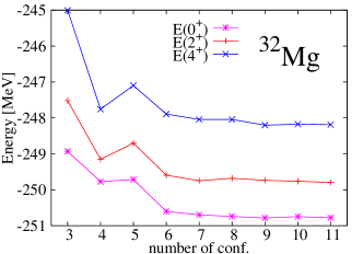
Figure 2: (Color online) Convergence of the $\beta_{2}$ configuration-mixing calculations for the $0^{+}$, $2^{+}$, and $4^{+}$ energies as the number of HFB states with different values of quadrupole moment chosen equidistantly in the range, $-80$ [fm${}^{2}]$ $\leq Q_{20}\leq$ 140 [fm${}^{2}]$, is increased.

In the actual calculations of $\beta_{2}$ configuration mixing, the quadrupole moment in Eq. (5) is constrained. Constraining the $\beta_{2}$ value is nontrivial because it depends on both the quadrupole moment and the radius. Figure 2 shows an example of convergence for the configuration-mixing calculation for ³²Mg as a function of the number of configurations. It can be seen that the results are stable for $N_{\beta_{2}}\mathrel{\mathchoice{\lower 3.6pt\vbox{\halign{$\mathsurround=0pt\displaystyle\hfil#\hfil$\cr>\crcr\sim\crcr}}}{\lower 3.6pt\vbox{\halign{$\mathsurround=0pt\textstyle\hfil#\hfil$\cr>\crcr\sim\crcr}}}{\lower 3.6pt\vbox{\halign{$\mathsurround=0pt\scriptstyle\hfil#\hfil$\cr>\crcr\sim\crcr}}}{\lower 3.6pt\vbox{\halign{$\mathsurround=0pt\scriptscriptstyle\hfil#\hfil$\cr>\crcr\sim\crcr}}}}8$, and thus we take $N_{\beta_{2}}=10$ in the following calculations. The deformation parameters of the HFB states employed are in the range of $-0.5\lesssim\beta_{2}\lesssim 0.8$, which mostly covers the important low-energy region of the potential energy curve, c.f. Sec. III.1. The sets of values, ($\beta_{2}^{(n)};n=1:10$), for the calculated Mg isotopes are shown in Table 1.

Nuclide	$\beta_{2}^{(n)};n=1:10$
24Mg	$-$0.45	$-$0.32	$-$0.15	0.04	0.23	0.41	0.55	0.66	0.75	0.83
26Mg	$-$0.50	$-$0.40	$-$0.26	0.07	0.12	0.30	0.45	0.58	0.69	0.78
28Mg	$-$0.49	$-$0.37	$-$0.21	0.02	0.19	0.37	0.52	0.65	0.75	0.83
30Mg	$-$0.52	$-$0.41	$-$0.27	0.09	0.11	0.30	0.47	0.60	0.71	0.80
32Mg	$-$0.49	$-$0.37	$-$0.23	0.05	0.13	0.31	0.46	0.60	0.70	0.79
34Mg	$-$0.49	$-$0.38	$-$0.23	0.05	0.14	0.32	0.48	0.60	0.72	0.82
36Mg	$-$0.50	$-$0.38	$-$0.23	0.04	0.15	0.33	0.48	0.61	0.73	0.82
38Mg	$-$0.50	$-$0.39	$-$0.24	0.06	0.13	0.31	0.46	0.59	0.70	0.79
40Mg	$-$0.50	$-$0.38	$-$0.24	0.05	0.14	0.32	0.46	0.60	0.70	0.79

Table 1: Parameter sets ($\beta_{2}^{(n)};n=1:10$) taken for $\beta_{2}$ configuration mixing.

The Hill–Wheeler equation suffers from the numerical problem of vanishing norm states RS80 . To avoid this, the eigenstates of the norm kernel whose eigenvalues are smaller than a certain value need to be excluded. This norm cutoff value needs to be as small as possible, and we normally set it to $10^{-10}$. However, we have found that this value is too small for calculations including $\beta_{2}$ configuration mixing with infinitesimal cranking in the nuclei ^24,26Mg, for which we use the larger value of $10^{-7}$.

III Results

We performed the following four kinds of beyond mean-field (BMF) calculations in addition to spherical and deformed HFB calculations in order to separately investigate the following effects: (i) $\beta_{2}$ deformation, (ii) restoration of the rotational symmetry by the AMP, (iii) $\beta_{2}$ configuration mixing (CM$\beta_{2}$), and (iv) infinitesimal cranking (CR).

1. BMF(AMP+CM$\beta_{2}$+CR): This is the full calculation that includes the effects of (i) to (iv) with the wave function

   $$|\Psi^{I}_{M}\rangle=\sum_{Kn}g^{I}_{Kn}\hat{P}^{I}_{MK}|\Phi_{\rm cr}(\beta_{2}^{(n)})\rangle.$$ (12)

2. BMF(AMP+CM$\beta_{2}$): This BMF calculation includes the effects of (i) to (iii) with the wave function

   $$|\Psi^{I}_{M}\rangle=\sum_{n}g^{I}_{0n}\hat{P}^{I}_{M0}|\Phi(\beta_{2}^{(n)})\rangle.$$ (13)

3. BMF(AMP+CR): This BMF calculation includes the effects of (i), (ii) and (iv) with the wave function

   $$|\Psi^{I}_{M}\rangle=\sum_{K}g^{I}_{K}\hat{P}^{I}_{MK}|\Phi_{\rm cr}(\beta_{2}^{\rm min})\rangle,$$ (14)

   where $\beta_{2}^{\rm min}$ is the value of $\beta_{2}$ which gives the minimum energy of the projected $0^{+}$ ground state.

4. BMF(AMP): This BMF calculation includes the effects of (i) and (ii) with the wave function

   $$|\Psi^{I}_{M}\rangle=g^{I}_{0}\hat{P}^{I}_{M0}|\Phi(\beta_{2}^{\rm min})\rangle,$$ (15)

   where the $\beta_{2}^{\rm min}$ value is the same as in Eq. (14) because the cranking frequency is infinitesimally small.

BMF(AMP+CM$\beta_{2}$) calculations were first performed for the axially symmetric deformation using the Gogny D1S force in Ref. RER02 . Although we confirmed their results, we present our BMF(AMP) and BMF(AMP+CM$\beta_{2}$) results in addition to BMF(AMP+CM$\beta_{2}$+CR) and BMF(AMP+CR) to aid the understanding in our discussion.

Number projection is not performed in the present work, and number conservation is treated approximately BDF89 by replacing the Hamiltonian $H\rightarrow H-\lambda_{\nu}(N-N_{0})-\lambda_{\pi}(Z-Z_{0})$, where $N_{0}$ and $Z_{0}$ are the neutron and proton numbers to be fixed, and the neutron and proton chemical potentials $\lambda_{\nu}$ and $\lambda_{\pi}$ are chosen to be those of the first ($n=1$) HFB state. We checked the expectation values of the numbers in the full BMF(AMP+CM$\beta_{2}$+CR) calculations. The average deviations $|\langle N-N_{0}\rangle|$ and $|\langle Z-Z_{0}\rangle|$ for the calculated cases are typically $0.02-0.08$, and the worst case is 0.19 for neutrons in ³⁸Mg, which is still less than 1% of $N_{0}$. Therefore the number conservation on average is maintained well in the configuration-mixing calculations. The neutron or proton pairing correlation vanishes depending on the quadrupole moment, or $\beta_{2}$ (see, e.g., Fig. 3 of Ref. RER02 ). The number fluctuations $\langle\Delta N^{2}\rangle$ and $\langle\Delta Z^{2}\rangle$ for the HFB states with non-vanishing pairing correlations are typically about $1.4-4$ for neutrons and about $1.2-3$ for protons. Thus, the pairing correlations are not very strong for these Mg isotopes, and variation after number projection may be necessary for better treatment of the pairing correlation, which is outside the scope of this work.

III.1 Energy surfaces

Figure 3 shows the ground-state potential energy curves obtained by deformed HFB (dashed line) and by BMF(AMP) (solid line) calculations for ³²Mg. The excited $2^{+}$ and $4^{+}$ states from the BMF(AMP+CR) calculations are also included (the deformed HFB and the BMF(AMP) $0^{+}$ state are not affected by infinitesimal cranking). Compared to the similar calculation in Ref. RER02 which did not include infinitesimal cranking, the $2^{+}$ and $4^{+}$ energy curves are considerably lower in energy, which shows the importance of the effect of time-odd components in the wave function. Although deformed-HFB calculations yield a minimum at $\beta_{2}=0$, large energy gains are obtained by BMF(AMP) calculations for finite $\beta_{2}$. Consequently, BMF(AMP) calculations suggest that a considerably large prolate deformation ($\beta_{2}\approx$ 0.42) is favored, which is consistent with the suggestion by the experiment in Refs. Moto95 ; Prit99 ; Chiste01 ; NNDC . Thus, it is quite important to perform AMP to obtain the correct value of nuclear deformation. The spherical barrier, which corresponds to the energy difference between the prolate and spherical states, is not very large ($\Delta E\approx 2.3$ MeV). An oblate minimum is found at $\beta_{2}\approx-0.23$, and the energy difference between the prolate and oblate states is $\Delta E\approx 870$ keV. These results indicate that this nucleus is soft with respect to $\beta_{2}$ deformation and that configuration mixing should therefore be taken into account.

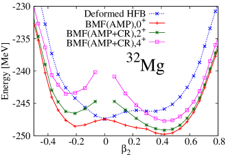
Figure 3: (Color online) Potential-energy curves by deformed HFB and BMF(AMP+CR) calculations for ³²Mg with the Gogny-D1S interaction. The ground-state ($I^{\pi}=0^{+}$) energy as well as excited $2^{+}$ and $4^{+}$ energies are plotted as a function of $\beta_{2}$.

Figure 4 shows the potential energy curves for ⁴⁰Mg. Again, the $2^{+}$ and $4^{+}$ energies are considerably lower in energy compared to Ref. RER02 . Prolate deformation is favored in both deformed HFB and BMF(AMP) calculations. In contrast to the case of ³²Mg, a considerably deep prolate minimum is obtained. The spherical barrier is large ($\Delta E\approx 5.7$ MeV). An oblate minimum is found at $\beta_{2}\approx-0.38$, and the energy difference between the prolate and oblate states is $\Delta E\approx 1.8$ MeV. Thus, the effects of $\beta_{2}$ configuration mixing may be small for ⁴⁰Mg.

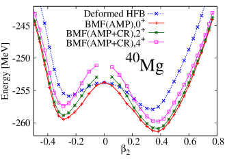
Figure 4: (Color online) Same as Fig. 3, but for ⁴⁰Mg.

We determine nuclear deformation from the $\beta_{2}$ value that yields an energy minimum. Figure 5 shows this value plotted against $A$ for deformed-HFB calculations (open squares) and BMF(AMP) calculations for the $0^{+}$ ground states (closed squares). The two results are quite different for ^30,32Mg. In the BMF(AMP) calculations, these $\beta_{2}^{\rm min}$ values are used for the HFB states, c.f. Eqs. (14) and (15). This shows that it is essential to determine it properly by calculations that restore the rotational symmetry, particularly around $A=32$ ($N=20$).

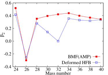
Figure 5: (Color online) Deformation parameters $\beta_{2}$ that yield energy minima in deformed-HFB and BMF(AMP) calculations versus mass number.

III.2 Matter radii

Figure 6 shows the rms matter radius $r_{\rm m}$ for the ground-state densities of Mg isotopes from $A=24$ to 40 as obtained by analysis of the reaction cross sections Takechi-Mg ; Watanabe14 . The finite-size effect of nucleons is subtracted from the experimental data. In the calculation, the center-of-mass correction has been performed by replacing the nucleon coordinate $r$ with $\mbox{\boldmath$r$}-\mbox{\boldmath$R$}$ where $R$ is the center-of-mass coordinate. Although this effect is small at about 1%, it is not completely negligible. The difference between deformed-HFB results (open triangles) and spherical-HFB results (open diamonds) is quite large, indicating that nuclear deformation plays an important role in $r_{\rm m}$. Our full BMF(AMP+CM$\beta_{2}$+CR) calculations (closed squares) yielded excellent agreement with the experimental data $r_{\rm m}^{\rm exp}$, compared to the deformed-HFB results. The four BMF results, that is, BMF(AMP+CM$\beta_{2}$+CR), BMF(AMP+CM$\beta_{2}$), BMF(AMP+CR), and BMF(AMP), are all similar. The non-negligible enhancement from deformed-HFB results to BMF(AMP+CM$\beta_{2}$+CR) results, particularly for ^30,32Mg, is thus thought to come mainly from the large change in the equilibrium deformation caused by the AMP as shown in Fig. 5. It should be noted that all of the multipole deformations contribute to increasing the nuclear radius. Although the effect of the quadrupole deformation is dominant in the present study of Mg isotopes, the hexadecapole deformation is non-negligible for most of the isotopes.

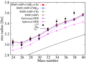
Figure 6: (Color online) Root mean square radii of Mg isotopes. Four results from BMF(AMP+CM$\beta_{2}$+CR), BMF(AMP+CM$\beta_{2}$), BMF(AMP+CR), and BMF(AMP) are shown by closed squares, open squares, open circles, open down-triangles, respectively. For comparison, deformed and spherical HFB results are also shown by open triangles and open diamonds, respectively. Experimental radii $r_{\rm m}^{\rm exp}$ are deduced from measured $\sigma_{\rm R}$ Watanabe14 ; Takechi-Mg . The solid line shows the empirical formula $r_{\rm m}^{\rm emp}=1.2A^{1/3}\sqrt{3/5}$ [fm] for the rms matter radius in the spherical limit that is obtained from a uniform density with a radius $1.2A^{1/3}$ [fm].

The empirical formula $1.2A^{1/3}$ [fm] is widely used for nuclear radii. The corresponding rms radius is also plotted as a solid line, which shows that the formula largely underestimates $r_{\rm m}^{\rm exp}$. The matter densities are thus much more extended than typical nuclear densities with radii $1.2A^{1/3}$ [fm] for even stable Mg isotopes. If the deformation parameter $\beta_{2}$ is deduced from measured quantities, it is necessary that $r_{\rm m}^{\rm exp}$ is available, as shown in Eq. (4). At least for lighter nuclei such as Mg isotopes, the empirical formula $r_{\rm m}^{\rm emp}=1.2A^{1/3}\sqrt{3/5}$ [fm] should not be used instead of $r_{\rm m}^{\rm exp}$, even if it is not available. This is discussed in Sec. III.3.

III.3 Transition probabilities

Figure 7 shows the results for the $E2$ transition probabilities $B(E2;0^{+}\rightarrow 2^{+})$ together with experimental data where available. No effective charge is required in our calculations. Comparing the four calculations BMF(AMP+CM$\beta_{2}$+CR), BMF(AMP+CM$\beta_{2}$), BMF(AMP+CR), and BMF(AMP), it can be seen that both $\beta_{2}$ configuration mixing and infinitesimal cranking yield non-negligible effects; those of the former (latter) is about $8\%-28\%$ ($7\%-14\%$). The combined effect on BMF(AMP) reduces the $B(E2)$ values by about $15\%-35\%$ except for ²⁶Mg, which is predicted to be oblate in its ground state, c.f. Fig. 5. These effects are much larger on $B(E2)$ than on $r_{\rm m}$. The BMF(AMP+CM$\beta_{2}$+CR) calculations thus agree quite well with the measured $B(E2)$ when we consider that our calculations have no adjustable parameters.

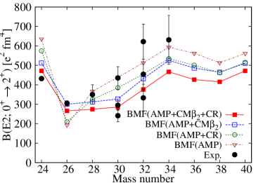
Figure 7: (Color online) $B(E2)$ transition probabilities of Mg isotopes. Four results of BMF(AMP+CM$\beta_{2}$+CR), BMF(AMP+CM$\beta_{2}$), BMF(AMP+CR), and BMF(AMP) calculations are compared with experimental data (“Exp.”) from Refs. Moto95 ; Prit99 ; Chiste01 ; Raman01 ; Nied05 ; Iwasaki01 .

The $B(E2)$ transition probability within the rotational band provides us with information on the quadrupole deformation parameter $\beta_{2}$. Although it is not directly observable and a model is needed to determine its value, this dimensionless quantity is quite useful and often employed in the analysis of experimental data. Reliable estimation of $\beta_{2}$ is thus meaningful and is described in the Appendix; see Table 2. In the Appendix, the absolute values of $\beta_{2}$ calculated from measured values of $B(E2)$ and $r_{\rm m}$ are compared with those obtained by replacing $r_{\rm m}$ with the empirical formula $r_{\rm m}^{\rm emp}=1.2A^{1/3}\sqrt{3/5}$ [fm], c.f. Fig. 11 in the Appendix. The latter values overestimate the former by about 20% because $r_{\rm m}^{\rm emp}$ underestimates the experimental $r_{\rm m}$ by about 10% as shown in Sec. III.2. This clearly indicates that simultaneous analysis of $B(E2)$ and $r_{\rm m}$ is important for estimating the deformation precisely, particular in order to avoid confusing the effects of deformation and expansion.

III.4 Excitation energies

The first $2^{+}$ and $4^{+}$ excitation energies $E(2^{+})$ and $E(4^{+})$ are shown in Fig. 8. The excitation energies from full BMF(AMP+CM$\beta_{2}$+CR) (filled squares) agree quite well with the experimental data. For ²⁴Mg, however, the results underestimate the experimental values. There are two possible reasons. One is that the pairing gaps for both neutrons and protons vanish around the projected minimum in the Gogny-D1S calculation, which makes the moment of inertia larger. Another possible reason is the effect of alpha clustering in ²⁴Mg. The results from BMF(AMP+CM$\beta_{2}$+CR) are rather different from those in Ref. RER02 where the effect of cranking is not included and the excitation energies are systematically larger, that is, the moments of inertia are smaller. Our results are consistent with Ref. RER15 where the configuration mixing for both $(\beta_{2},\gamma)$ deformation and cranking frequency is taken into account. This agreement indicates that the effect of triaxial deformation might not be very important, at least for the low-lying states of the Mg isotopes.

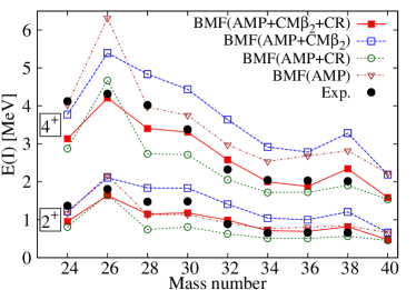
Figure 8: (Color online) Excitation energies $E(2^{+})$ and $E(4^{+})$ of Mg isotopes. Four results of BMF(AMP+CM$\beta_{2}$+CR), BMF(AMP+CM$\beta_{2}$), BMF(AMP+CR), and BMF(AMP) calculations are compared with experimental data (“Exp.”) from Refs. NNDC ; Door13 and references therein.

In contrast to the full BMF(AMP+CM$\beta_{2}$+CR) calculations, the excitation energies from BMF(AMP+CR) (open circles) are systematically lower than the experimental data. The $\beta_{2}$-configuration mixing thus considerably increases the excitation energies of the $2^{+}$ and $4^{+}$ states. However, the results from BMF(AMP+CM$\beta_{2}$) (open squares) greatly overestimate the experimental data. This clearly shows that the effects of the time-odd components induced by the infinitesimal cranking procedure are very important. The effect of cranking induces $K$-mixing in the wave function as shown in Eqs. (12)–(15), which, as a result, reduces the energies of the $2^{+}$ and $4^{+}$ states but not the $0^{+}$ state in which there is no $K$-mixing. Therefore, the effects of both $\beta_{2}$ configuration mixing and infinitesimal cranking are important for reproducing excitation energies for the $2^{+}$ and $4^{+}$ states of the ground-state rotational band. The simplest BMF(AMP) almost reproduces the $2^{+}$ excitation energies accidentally in these Mg isotopes. The $4^{+}$ energies, however, are overestimated considerably, and thus the BMF(AMP) calculation does not describe the data very well.

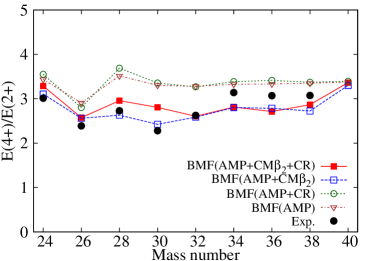
Figure 9: (Color online) Ratios $E(4^{+})/E(2^{+})$ for Mg isotopes. The results of BMF(AMP+CM$\beta_{2}$+CR), BMF(AMP+CM$\beta_{2}$) BMF(AMP+CR), and BMF(AMP) calculations are compared.

The ratios $E(4^{+})/E(2^{+})$ are shown in Fig. 9. The BMF(AMP+CM$\beta_{2}$) results without cranking agree quite well with the experimental values, although the energy is spaced too widely as can be seen in Fig. 8. Both the BMF(AMP) and BMF(AMP+CR) results without $\beta_{2}$ configuration mixing give values around the ideal rotational ratio of 3.3. Inclusion of the effects of $\beta_{2}$-fluctuations reduces the ratio, which clearly indicates that the effects of the $\beta_{2}$-fluctuation included by the $\beta_{2}$ configuration mixing are very important for describing the deviation from the ideal rotational behavior. The ideal ratio of the vibrational motion is $E(4^{+})/E(2^{+})=2$, which is closer to the experimental data for ^26,30Mg. However, comparing the results of BMF(AMP+CM$\beta_{2}$+CR) and BMF(AMP+CM$\beta_{2}$), it can be seen that the infinitesimal cranking does not affect the ratio very much. The effect of infinitesimal cranking reduces the excitation energies, but keeps the ratio constant. That is, it only increases the moment of inertia without changing the properties of the rotational motion. The $\beta_{2}$-configuration mixing describes the deviation from the ideal rotational motion and has a large influence on the ratio $E(4^{+})/E(2^{+})$.

Figure 10 shows the probability distributions of the $0^{+},2^{+}$ and $4^{+}$ states by full BMF(AMP+CM$\beta_{2}$+CR) calculations. For nuclei ^24,34,40Mg, the distributions of the $0^{+}$, $2^{+}$ and $4^{+}$ states are well located in the prolate deformation side. With the exception of ²⁶Mg, the distributions of excited states are also located on the prolate side. However, the distribution of the ground state is spread across both the oblate and prolate sides for most nuclei. In particular, an almost uniform distribution is seen in the wide range around the spherical shape for the $0^{+}$ state in ³⁰Mg. This indicates that both the prolate and oblate configurations contribute to the ground-state wave function. For the nucleus ²⁶Mg, an interesting transition in the distribution occurs from the oblate to prolate side in which the majority of mixing probabilities are on the oblate side in the ground state whereas they are on the prolate side in the $4^{+}$ state. Comparing the distributions of BMF(AMP+CM$\beta_{2}$+CR) calculations with the those of BMF(AMP+CM$\beta_{2}$) calculations (not shown) shows that they are quite similar to each other, although there is a slight change in the $2^{+}$ and $4^{+}$ distributions for ^26-30Mg nuclei. Since infinitesimal cranking does not affect the $0^{+}$ state, there is no effect on the $0^{+}$ distributions.

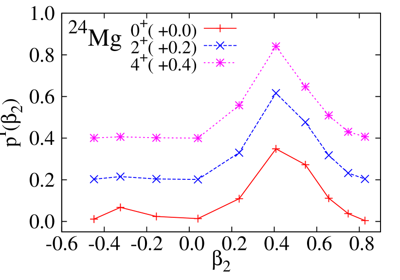
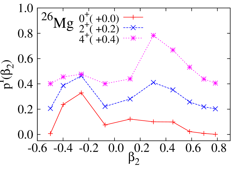
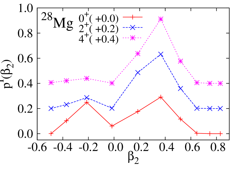
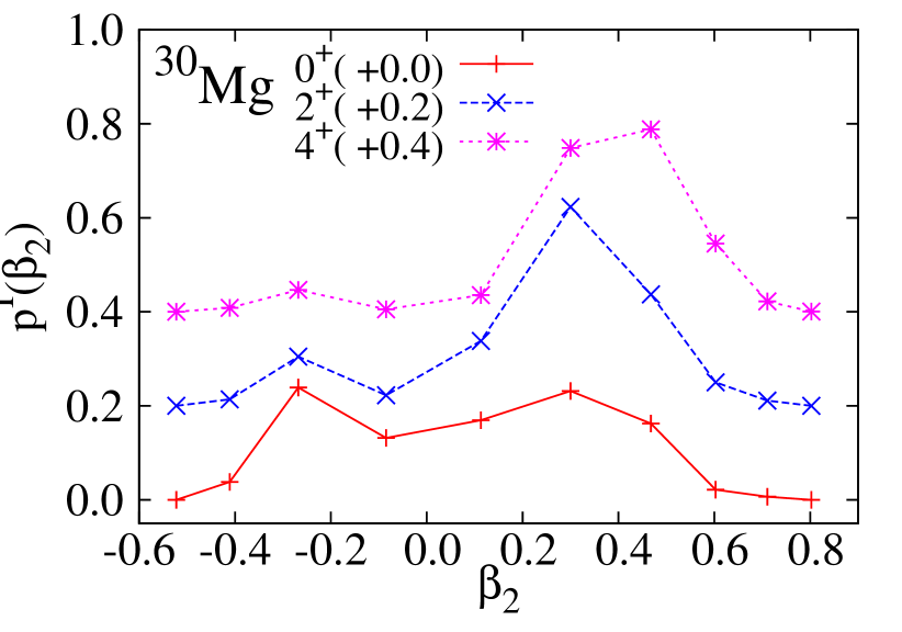
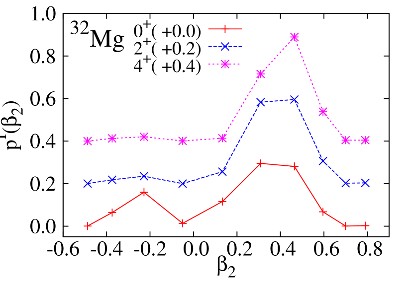
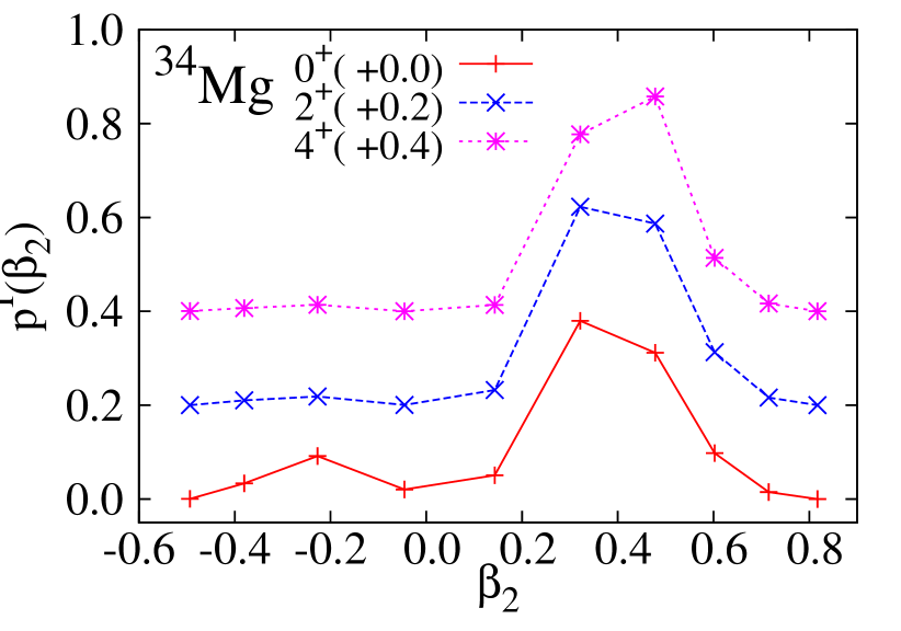
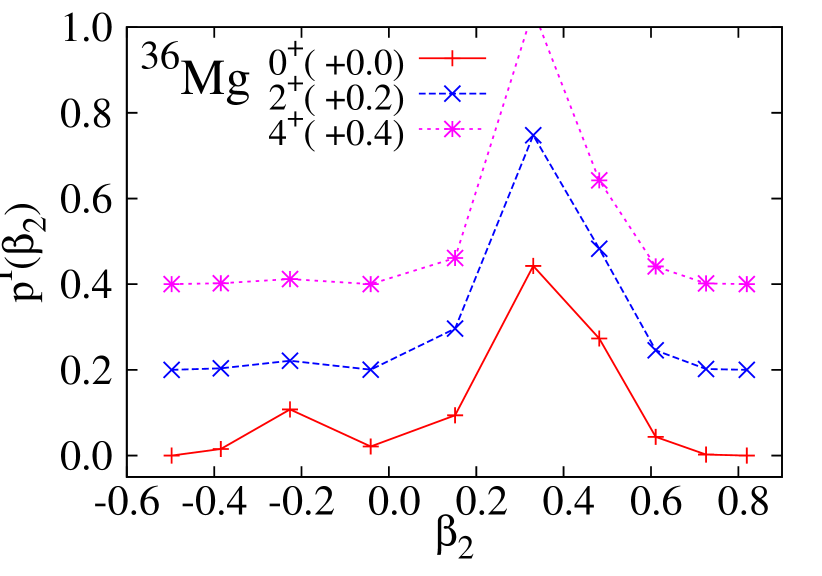
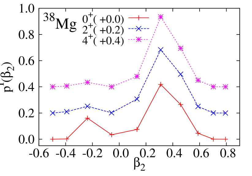
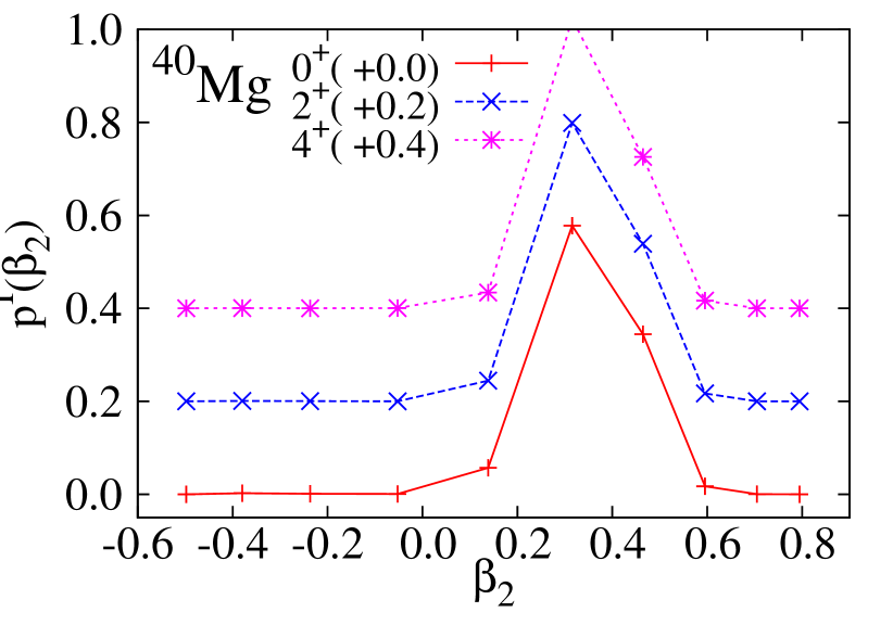
Figure 10: (Color online) Probability distributions from BMF(AMP+CM$\beta_{2}$+CR) calculations for the $0^{+},2^{+}$ and $4^{+}$ states of Mg isotopes. The corresponding distributions are shifted by $+0.2$ and $+0.4$ for the $2^{+}$ and $4^{+}$ states, respectively.

IV Summary

In this paper, we simultaneously analyzed the three observables $r_{\rm m}$, $B(E2)$, and $E(2^{+})$ and $E(4^{+})$ for ^24-40Mg using the BMF framework with angular-momentum-projected configuration mixing with infinitesimal cranking TS16 . The present BMF results are consistent with the results of state-of-the-art BMF calculations in Ref. RER15 for $E(2^{+})$ and $E(4^{+})$ in ^24-34Mg, and with the experimental data. Very recently, Ref. TS16 showed that infinitesimal cranking gives a practical and good description of low-lying states. The present BMF framework is thus considered to be practical and rather reliable. In fact, the present BMF calculations successfully reproduce all of the data for $r_{\rm m}$, $B(E2)$ and $E(2^{+})$ and $E(4^{+})$. We thus conclude that the present BMF framework is quite useful for data analysis, particularly for low-lying states.

We deduced the absolute value of the experimental deformation parameter $\beta_{2}$ from measured values of $B(E2)$ and $r_{\rm m}$, and present the resultant values in Table 2 in the Appendix. Although the $\beta_{2}$ parameter is not directly measurable, the present BMF framework is useful for extracting the values of $\beta_{2}$. By comparing the values extracted from $B(E2)$ and $r_{\rm m}$ and from measured $B(E2)$ and the empirical formula $r_{\rm m}^{\rm emp}=1.2A^{1/3}\sqrt{3/5}$ [fm], we show that the latter overestimates the former by about 20%, since $r_{\rm m}^{\rm emp}$ underestimates $r_{\rm m}^{\rm exp}$ by about 10%. This clearly shows that simultaneous analysis of $r_{\rm m}$ and $B(E2)$ is quite important not only for determining the deformation parameter precisely but also for confirming the reliability of the theoretical framework.

We performed a detailed analysis by using the BMF framework which imposes the restrictions that the system is axially symmetric and parity conserving. The present BMF framework can take account of the following four effects, separately: (i) $\beta_{2}$ deformation, (ii) change in $\beta_{2}$ by AMP from the minimum of HFB energy surface to that of projected-energy surface, (iii) configuration mixing for axially symmetric $\beta_{2}$ deformation, and (iv) inclusion of time-odd components by the cranking procedure. Important effects are (i) and (ii) for $r_{\rm m}$ and (i) to (iv) for both $B(E2)$ and $(E(2^{+}),E(4^{+}))$. The effect (iv) especially reduces the values of $E(2^{+})$ and $E(4^{+})$ without changing the ratio $E(4^{+})/E(2^{+})$. The effect (iv) thus enlarges the moment of inertia. We thus propose that BMF(AMP) calculations with effects (i) and (ii) are useful for analysis of the matter radii, and full BMF(AMP+CM$\beta_{2}$+CR) calculations with effects (i) to (iv) are useful for both the transition probabilities and the excitation energies.

*

Appendix A Deformation parameter $\beta_{2}$

In this appendix, we discuss the values of the deformation parameter $\beta_{2}$ extracted from the measured $B(E2)$ and $r_{m}$. For this purpose the quadrupole moment $Q_{20}$ in Eq. (4) is expected to be related to $B(E2)$, for which the rotor model is necessary (see, e.g., Ref. RS80 ). However, the validity of the rotor model is questionable especially for the case of smaller deformations in lighter systems. Ref. RB12 gives a condition for the validity of the rotor model for $B(E2)$, Eq. (16); i.e., the angular-momentum fluctuation $\langle\Delta J^{2}\rangle$ for the HFB state, from which the AMP is performed, is larger than about 15$\hbar^{2}$. In the present case, although the Mg isotopes are rather light, the resultant deformations are relatively large, c.f. Table 2. We checked that $\langle\Delta J^{2}\rangle\mathrel{\mathchoice{\lower 3.6pt\vbox{\halign{$\mathsurround=0pt\displaystyle\hfil#\hfil$\cr>\crcr\sim\crcr}}}{\lower 3.6pt\vbox{\halign{$\mathsurround=0pt\textstyle\hfil#\hfil$\cr>\crcr\sim\crcr}}}{\lower 3.6pt\vbox{\halign{$\mathsurround=0pt\scriptstyle\hfil#\hfil$\cr>\crcr\sim\crcr}}}{\lower 3.6pt\vbox{\halign{$\mathsurround=0pt\scriptscriptstyle\hfil#\hfil$\cr>\crcr\sim\crcr}}}}18-35\hbar^{2}$ for the HFB states with deformation $|\beta_{2}|\approx 0.35-0.45$. We therefore think that the rotor model can be applied quite safely. Thus, according to the rotor model expression of $B(E2)$,

$$B_{\rm rot}(\mathrm{E}2;I_{i}\rightarrow I_{f})=\langle I_{i}020|I_{f}0\rangle(Q^{(E)}_{20})^{2},$$ (16)

where $Q^{(E)}_{20}$ is the electric quadrupole moment. The mass quadrupole moment is extracted from the observed $B(E2)$ value

$$|Q_{20}|=\frac{A}{Ze}\sqrt{B(E2;0^{+}\rightarrow 2^{+})},$$ (17)

assuming the same deformation for neutrons and protons. In this way, we extract the deformation parameters $|\beta_{2}|$ if experimental $r_{\rm m}$ are available, as tabulated in Table 2.

Nuclide	$|\beta_{2}|$	Error	$~{}~{}{\rm Ref.~{}for~{}}B(E2)$
24Mg	0.474	0.026	Raman01
26Mg	0.409	0.014	Raman01
28Mg	0.403	0.031	Raman01
30Mg	0.336	0.023	Nied05
30Mg	0.372	0.018	Prit99
30Mg	0.452	0.031	Chiste01
32Mg	0.410	0.036	Moto95
32Mg	0.351	0.037	Prit99
32Mg	0.480	0.035	Chiste01
34Mg	0.445	0.046	Iwasaki01

Table 2: $|\beta_{2}|$ values obtained from measured values of $B(E2)$ and $r_{\rm m}$ by Eq. (4) with (17).

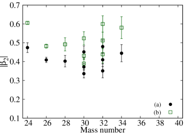
Figure 11: (Color online) Absolute values of (a) experimental and (b) empirical $\beta_{2}$ values. Experimental $|\beta_{2}|$ (solid squares) are obtained using Eqs. (4) and (17) from measured values of $B(E2)$ and $r_{\rm m}$, while empirical $|\beta_{2}|$ (open squares) are evaluated from measured $B(E2)$ and empirical radii $r_{\rm m}^{\rm emp}=1.2A^{1/3}\sqrt{3/5}$ [fm].

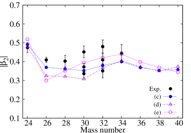
Figure 12: (Color online) Absolute values of three kinds of theoretical $\beta_{2}$ parameters: (c) $|\beta_{2}|$ obtained using Eqs. (4) and (17) from the results of full BMF(AMP+CM$\beta_{2}$+CR) for $B(E2)$ and $r_{\rm m}$ (solid circles); (d) mean $\beta_{2}$ values (${\bar{\beta}}_{2}$) of Eq. (10) (open triangles); and (e) $\beta_{2}$ values that give a minimum of projected energy surface (open circles). These values are compared with the experimental $|\beta_{2}|$ values.

Figure 11 compares (a) the absolute values of $\beta_{2}$ extracted from measured $B(E2)$ and $r_{\rm m}$(solid circles) with (b) values from measured $B(E2)$ and empirical radius $1.2A^{1/3}$ (open squares), respectively, for $A=24-34$ Mg isotopes. The $|\beta_{2}|$ values assuming the empirical radii (b) overestimate those extracted from the measured radii (a) by about 20% because the empirical radii underestimate the measured values by about 10% as shown in Fig. 1. This clearly indicates that simultaneous analysis of $B(E2)$ and $r_{\rm m}$ is important for estimating the deformation reliably. Figure 12 shows the $A$ dependence of three kinds of theoretical $\beta_{2}$ parameters: (c) $|\beta_{2}|$ deduced from the results of full BMF(AMP+CM$\beta_{2}$+CR) calculations for $B(E2)$ and $r_{\rm m}$ (solid circles); (d) mean $\beta_{2}$ values (${\bar{\beta}}_{2}$) defined by Eq. (10) (open triangles); and (e) $\beta_{2}$ values corresponding to the minimum of the $0^{+}$ energy surface obtained by BMF(AMP) calculations (open circles), c.f., Sec. III.1 for details. The $|\beta_{2}|$ values of BMF(AMP+CM$\beta_{2}$+CR) (c) reproduce the experimental data quite well. The $|\beta_{2}|$ (d) also account for the experimental data well except for ^26-30Mg. For ^26-30Mg, the probability distributions are spread quite widely across both the oblate and prolate sides of $\beta_{2}$ with non-negligible probability in small deformation as shown in Fig. 10. This leads to effective reduction of deformation, and consequently the $|\beta_{2}|$ (d) slightly underestimates the experimental data. The $|\beta_{2}|$ (e) corresponding to the minimum of the projected energy surface is slightly different from BMF(AMP+CM$\beta_{2}$+CR), which shows the effect of configuration mixing.

References

- (1) M. Takechi et al., Phys. Rev. C 90, 061305(R) (2014).
- (2) S. Watanabe et al., Phys. Rev. C 89, 044610 (2014).
- (3) O. Sorlin and M.-G. Porquet, Prog. Part. Nucl. Phys. 61, 602 (2008).
- (4) I. Hamamoto, Phys. Rev. C 85, 064329 (2012).
- (5) P. Doornenbal et al., Phys. Rev. Lett. 111, 212502 (2013).
- (6) N. Kobayashi et al., Phys. Rev. Lett. 112, 242501 (2014).
- (7) E. Caurier et al., Phys. Rev. C 90, 014302 (2014).
- (8) T. Motobayashi et al., Phys. Lett. B 346, 9 (1995).
- (9) B.V. Pritychenko et al., Phys. Lett. B 461, 322 (1999).
- (10) V. Chist et al., Phys. Lett. B 514, 233 (2001).
- (11) Brookhaven database, http://www.nndc.bnl.gov.
- (12) K. Minomo, T. Sumi, M. Kimura, K. Ogata, Y. R. Shimizu, and M. Yahiro, Phys. Rev. C 84, 034602 (2011).
- (13) K. Minomo, T. Sumi, M. Kimura, K. Ogata, Y. R. Shimizu, and M. Yahiro, Phys. Rev. Lett. 108, 052503 (2012).
- (14) T. Sumi, K. Minomo, S. Tagami, M. Kimura, T. Matsumoto, K. Ogata, Y. R. Shimizu, and M. Yahiro, Phys. Rev. C 85, 064613 (2012).
- (15) J. Dechargé and D. Gogny, Phys. Rev. C 21, 1568 (1980).
- (16) J. F. Berger, M. Girod, and D. Gogny, Comput. Phys. Commun. 63, 365 (1991).
- (17) J. Terasaki, H. Flocard, P.-H. Heenen, and P. Bonche, Nucl. Phys. A 621, 706 (1997).
- (18) G. A. Lalazissis, A. R. Farhan, and M. M. Sharma, Nucl. Phys. A 628, 221 (1998).
- (19) R.-G. Reinhard, D. J. Dean, W. Nazarewicz, J. Dobaczewski, J. A. Maruhn, and M. R. Strayer, Phys. Rev. C 60, 014316 (1999).
- (20) B. Bastin et al., Phys. Rev. Lett. 99, 022503 (2007).
- (21) S. Takeuchi et al., Phys. Rev. Lett. 109, 182501 (2012).
- (22) M. Borrajo, T. R. Rodríguez, J. L. Egido, Phys. Lett. B 746, 341 (2015).
- (23) J. M. Yao, H. Mei, H. Chen, J. Meng, P. Ring, and D. Vretenar, Phys. Rev. C 83, 014308 (2011).
- (24) S. Tagami and Y. R. Shimizu, Phys. Rev. C 93, 024323 (2016).
- (25) P. Ring and P. Schuck, The Nuclear Many-Body Problem, Springer, New York (1980).
- (26) P. Bonche, J. Dobaczewski, H. Flocard, P.-H. Heenen, and J. Meyer, Nucl. Phys. A 510, 466 (1989).
- (27) A. Staszczak, M.Stoitsov, A. Baran, and W. Nazarewicz, Eur. Phys. J. A 46, 85 (2010).
- (28) S. Tagami and Y. R. Shimizu, Prog. Theor. Phys. 127, 79 (2012).
- (29) M. Shimada, S. Tagami, and Y. R. Shimizu, Prog. Theor. Exp. Phys. 2015, 063D02 (2015).
- (30) M. Shimada, S. Tagami, and Y. R. Shimizu, Phys. Rev. C 93, 044317 (2016).
- (31) R. Rodríguez-Guzmán 1, J. L. Egido, and L. M. Robledo, Nucl. Phys. A 709, 201 (2002).
- (32) S. Raman, C.W. Nestor, JR. and P. Tikkanen, At. Data Nucl. Data Tables 78, 1 (2001).
- (33) O. Niedermaier et al., Phys. Rev. Lett. 94, 172501 (2005).
- (34) H. Iwasaki et al., Phys. Lett. B 522, 227 (2001).
- (35) L. M. Robledo and G. F. Bertsch, Phys. Rev. C 86, 054306 (2012).