Emergence of Persistent Infection due to Heterogeneity

Abstract

We explore the emergence of persistent infection in a patch of population, where the disease progression of the individuals is given by the SIRS model and an individual becomes infected on contact with another infected individual. We investigate the persistence of contagion qualitatively and quantitatively, under varying degrees of heterogeneity in the initial population. We observe that when the initial population is uniform, consisting of individuals at the same stage of disease progression, infection arising from a contagious seed does not persist. However when the initial population consists of randomly distributed refractory and susceptible individuals, a single source of infection can lead to sustained infection in the population, as heterogeneity facilitates the de-synchronization of the phases in the disease cycle of the individuals. We also show how the average size of the window of persistence of infection depends on the degree of heterogeneity in the initial composition of the population. In particular, we show that the infection eventually dies out when the entire initial population is susceptible, while even a few susceptibles among an heterogeneous refractory population gives rise to a large persistent infected set.

I Introduction

How a disease spreads in a population is a question of much interest and relevance, and consequently has been extensively explored over the years McEvedy ; kaplan ; cliff . Mathematically, epidemiological models have successfully captured the dynamics of infectious disease murray ; edelstein ; CA1 ; sw ; scalefree ; network . One well known model for non-fatal communicable disease progression is the SIRS cycle. This model appropriately describes the progression of diseases such as small pox, tetanus, influenza, typhoid fever, cholera and tuberculosis hethcote ; ozcaglar .

The SIRS cycle is described by the following stages. At the outset an individual is susceptible to infection (a stage denoted by S). On being infected by contact with other infected people in the neighbourhood, the individual moves on to the infectious stage (denoted by I). This is followed by a refractory stage (denoted by R). In the refractory stage the individual becomes immune to disease and also does not infect others. But this immunity is temporary as the individual becomes susceptible again after some time interval.

Specifically, in this work we consider a cellular automata model of the SIRS cycle described above kuperman ; gade ; kohar . In this model of disease progression, time $t$ evolves in discrete steps, with each individual, indexed by $(i,j)$ on a $2$ dimensional lattice, characterized by a counter

$\tau_{i,j}(t)=0,1,\dots,\tau_{I}+\tau_{R}$

describing its phase in the cycle of the disease kuperman . Here $\tau_{I}+\tau_{R}=\tau_{0}$, where $\tau_{0}$ signifies the total length of the disease cycle. At any instant of time t, if phase $\tau_{i,j}$(t) = $0$, then the individual at site $(i,j)$ is susceptible; if $1\leq\tau_{i,j}(t)\leq\tau_{I}$, then it is infected; if phase $\tau_{i,j}(t)>\tau_{I}$, it is in the refractory stage. For, phase $\tau_{i,j}(t)\neq 0$ the dynamics is given by the counter updating by $1$ every time step, and at the end of the refractory period the individual becomes susceptible again, which implies if $\tau_{i,j}(t)=\tau_{0}$ then, $\tau_{i,j}(t+1)=0$. Namely:

$$\tau_{i,j}(t+1)=\begin{cases}\tau_{i,j}(t)+1&\text{ : }1\leq\tau_{i,j}(t)<\tau_{0}\\ 0&\text{ : }\tau_{i,j}(t)=\tau_{0}\end{cases}$$

Hence the disease progression is a cycle (see Fig.1). We consider the typical condition where the refractory period is longer than the infective stage, i.e. $\tau_{R}>\tau_{I}$.

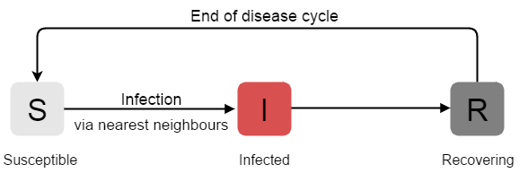
Figure 1: Schematic Representation of the SIRS cycle. The color scheme in all figures is as follows: black represents the refractory state (R); white represents the susceptible state (S); red represents the infected state (I).

We now investigate the spread of epidemic in a group of spatially distributed individuals, where at the individual level the disease progresses in accordance with the SIRS cycle. In particular, we consider a population of individuals on a $2$-dimensional lattice where every node, representing the individual, has $4$ neighbors rhodes . Unlike many studies with periodic boundary conditions, here the boundaries are fixed and there are no individuals outside the boundaries. So our model mimics a patch of population, and investigates the persistence of infection in such a patch.

Condition for infection: Here we consider the condition that a susceptible individual (S) will become infected (I) if one or more of its nearest neighbours are infected. That is, if $\tau_{i,j}(t)=0$, (namely, the individual is susceptible), then $\tau_{i,j}(t+1)=1$, if any $1\leq\tau_{x,y}(t)\leq\tau_{I}$ where $x,y\in\{(i-1,j);(i+1,j);(i,j-1);(i,j+1)\}$.

II Spatio-temporal patterns of infection spreading

We first focus on the infection spreading patterns in the population. The principal question we ask is the following: when is infection persistent in a patch, and how this depends on the constitution of the initial population. In order to examine this, we study the spread of infection from a seed of infection (namely one or two infected individuals) across a patch of population composed of individuals at different stages in the disease cycle, and with varying degrees of heterogeneity in the population.

With no loss of generality we consider $\tau_{I}=4$; $\tau_{R}=9$; $\tau_{0}=13$ and a lattice of size $100\times 100$. In our figures we represent the state of an individual in the disease cycle (namely S, I or R) by a color, with white denoting a susceptible individual, black denoting a refractory individual and red denoting an infected individual. The fraction of susceptible individuals in the population at time $t$ is denoted by $S_{t}$, the fraction of infected individuals by $I_{t}$ and the fraction of refractory individuals by $R_{t}$. In the sections below we will focus on the possibility of the prolonged existence of infection arising in different classes of initial populations, characterized by different $S_{0}$, $R_{0}$ and $I_{0}$.

II.1 Non-persistent Infection in a Homogeneous Susceptible Population

First we investigate the effect of an infected individual on a population patch where all individuals are entirely susceptible to infection. Namely, we consider the case where at the outset there is one infected individual and the rest of the population is in the susceptible state, with $\tau_{ij}=0$. Fig. 2 displays the spreading patterns obtained in such a scenario. It is clearly evident that as time progresses the infection starts from the infected individual (“seed”) and spreads symmetrically. This symmetric spreading pattern is readily understood from the condition for infection, which turns susceptible individuals to infected if any one of their neighbors is infected. So the infected seed infects its four neighbors, and these newly infected individuals in turn infect their nearest four neighbours, and so on. This process leads to an isotropic wave of infection which stops at the boundaries. We confirmed the generality of these observations for different relative lengths of the infectious and refractory periods, namely varying $\tau_{I}$ and $\tau_{R}$ (with $\tau_{I}<\tau_{R}$). We further ascertained that the choice of the location of the infected individual did not affect these qualitative trends.

Now the key factor in infection spreading is the contact of susceptible individuals with infected ones. It is clear that such an interaction takes place only at the outer edge of the wave of infection, while the inner boundary of the infected zone is contiguous only to refractory individuals. So the infection only spreads outwards, and does not move back into the interior of the lattice again. Importantly then, the infection is removed after a while from the patch of population, and all the individuals (including the original infective seed) comes to the end of the disease cycle and becomes susceptible again. So there is no infective site left in the population to perpetuate the infection and initiate another wave of disease spreading. Thus a fully susceptible population does not allow the infection to persist.

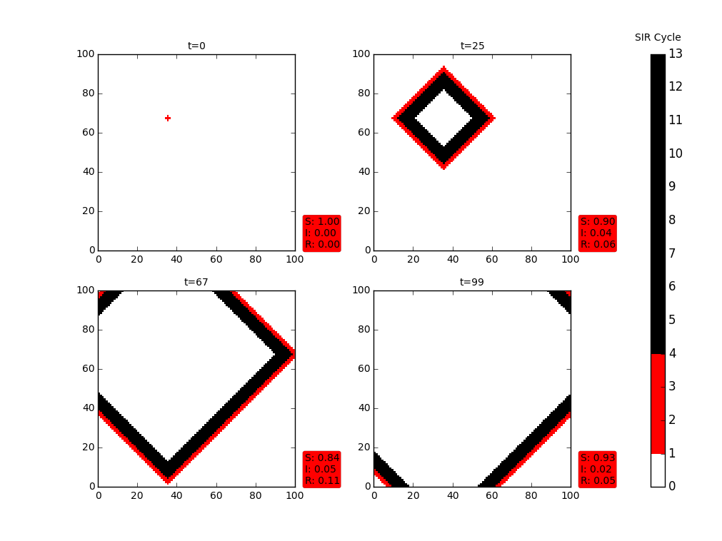
Figure 2: Snapshots at times $t=0,25,67,99$, showing the spread of infection from one infected individual at $t=0$, in a homogeneous initial population comprising entirely of susceptible individuals (i.e. $S_{0}\sim 1$, $R_{0}=0$, $I_{0}\sim 0$). The long bar shows the relative lengths of the susceptible (S), infected (I) and refractory (R) stages in the disease cycle, where $\tau_{I}=4$, $\tau_{R}=9$ and the total disease cycle $\tau_{0}$ is $13$ (see text). The red box shows the fraction of S, I and R individuals in the population at that instant of time.

II.2 Persistent infection in Heterogeneous Populations

Next we investigate the infection spread in the more realistic scenario where both refractory ($\tau_{i,j}>\tau_{I}$) and susceptible individuals ($\tau_{i,j}=0$) are present in the initial population, and are randomly distributed spatially. We first consider the case where the refractory individuals have phases $\tau_{i,j}=\tau_{I}+1$, namely, they are at the start of the refractory stage of the disease cycle. We investigate the persistence of infection in heterogeneous populations, with the initial state having (a) a single seed of infection and (b) varying initial fractions of infected individuals $(I_{0})$. In both scenarios, we analyze the effect of varying $S_{0}$ and $R_{0}$ on the persistence of infection.

To begin with, in Fig. 3, we illustrate the effect of a single infected individual on an initial population with equal numbers of susceptible and refractory individuals, namely $S_{0}=R_{0}$. It is evident from these representative results that in a well mixed population, consisting of a random collection of both susceptible and refractory individuals, introduction of a single infected individual can lead to persistent infection in the population.

This can be rationalized as follows: the mixed presence of susceptible and refractory individuals, implies that the disease cycles of the individuals in the population are not synchronized. So there are always some individuals in the infective stage of the disease cycle in the population, and these act as seeds for continued infection propagation, leading to persistent infection. Counter-intuitively then, the presence of individuals who are (temporarily) immune to the disease amongst susceptible ones leads to sustained infection, while in a completely susceptible population the infection dies out.

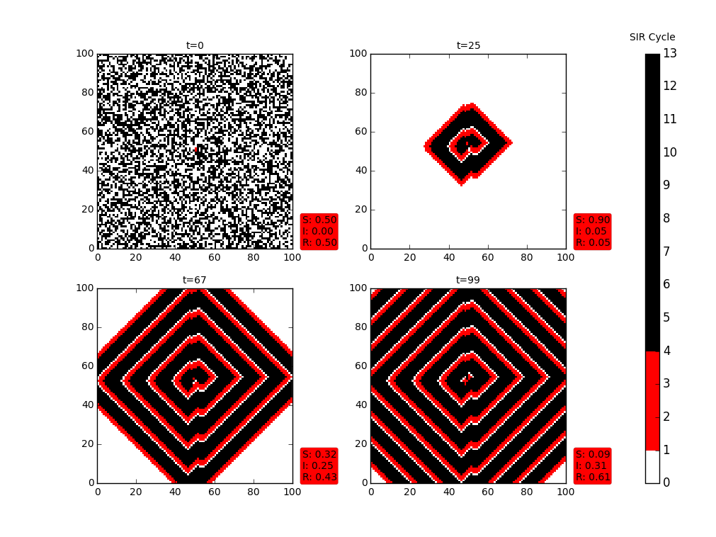
Figure 3: Snapshots of the infection spreading pattern in a heterogeneous population comprising initially of a random mixture of equal numbers of susceptible and refractory individuals ($S_{0}\sim 0.5$, $R_{0}\sim 0.5$ and $I_{0}\sim 0$), with one infected individual at $t=0$. Here the refractory individuals have phases $\tau_{i,j}=\tau_{I}+1$ (namely, they are at the start of the refractory stage of the disease cycle). Again, the long bar shows the relative lengths of the susceptible (S), infected (I) and refractory (R) stages in the disease cycle, where $\tau_{I}=4$, $\tau_{R}=9$ and the total disease cycle $\tau_{0}$ is $13$ (see text). The red box shows the fraction of S, I and R individuals in the population at that instant of time. Interestingly, the spatially random population evolves into a more regular pattern after a short transient time.

Next we focus on the time evolution of an initial population consisting of a random mixture of $S$, $I$ and $R$ states. In particular we investigate the nature of the persistent infection in the population under varying initial fractions of infected individuals $I_{0}$. A typical random initial condition is shown in Fig. 4, with the initial fraction of infected sites $I_{0}$ being one-tenth and the initial fraction of susceptibile and refractory individuals being equal (i.e. $S_{0}=R_{0}$). Here too we find that infection is sustained.

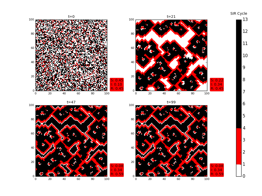
Figure 4: Snapshots of the infection spreading pattern in a heterogeneous population comprising initially of a random mixture of individuals, with $S_{0}=R_{0}$ and $I_{0}=0.1$. Here the refractory individuals have phases $\tau_{i,j}=\tau_{I}+1$ (namely, they are at the start of the refractory stage of the disease cycle). Again, the long bar shows the relative lengths of the susceptible (S), infected (I) and refractory (R) stages in the disease cycle, where $\tau_{I}=4$, $\tau_{R}=9$ and the total disease cycle $\tau_{0}$ is $13$ (see text). The red box shows the fraction of S, I and R individuals in the population at that instant of time.

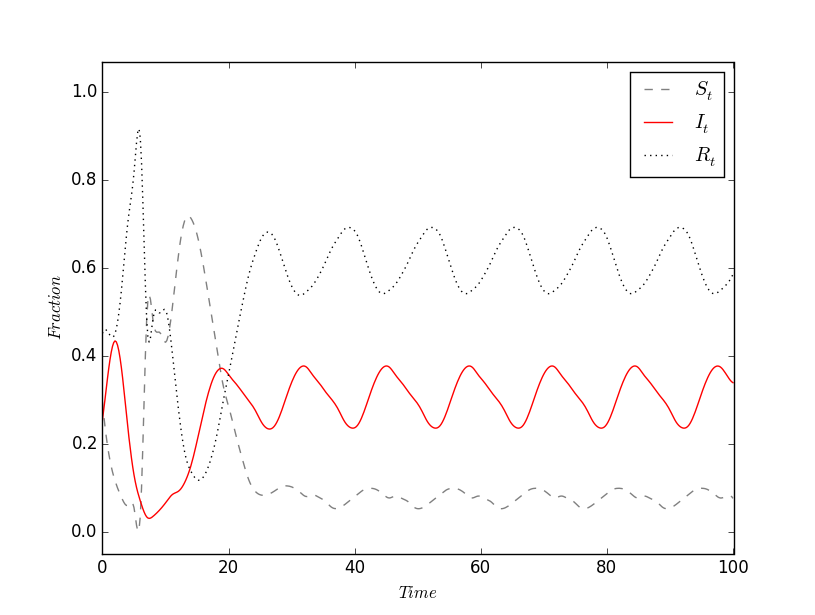
Figure 5: Time evolution of $I_{t}$, $S_{t}$, $R_{t}$, in a heterogeneous population comprising initially of a random mixture of individuals, with $S_{0}=R_{0}$ and $I_{0}=0.1$.

Further, interestingly, it is clear that there is an approximate recurrence of the complex patterns of infected individuals in the population. Fig. 5 shows the time evolution of the fraction of infected, refractory and susceptible individuals in the population, namely $I_{t}$, $R_{t}$ and $S_{t}$, in the case displayed in Fig. 4. It can be clearly seen that after transience, $I_{t}$, $R_{t}$ and $S_{t}$ exhibit steady oscillatory dynamics, with period of oscillation close to the disease cycle length $\tau_{0}$. This is consistent with the observed recurrence of the spatio-temporal patterns when persistent infection emerges.

A quantitative measure of the recurrence of patterns can also be obtained by calculating the difference of the state of the population from the initial state, as reflected by the Hamming distance:

$$H=\frac{1}{N}\sum_{i,j}\lvert\tau_{i,j}(t)-\tau_{i,j}(0)\rvert$$ (1)

where the sum is over all $N$ sites in the lattice. The time dependence of the Hamming distance given above is shown in Fig. 6, and it clearly shows steady oscillations. This indicates that the fraction of the susceptible, infected and refractory individuals in the population, and more remarkably their locations, repeat almost periodically over time. It should be noted that the frequency of oscillation again approximately corresponds to the disease cycle length.

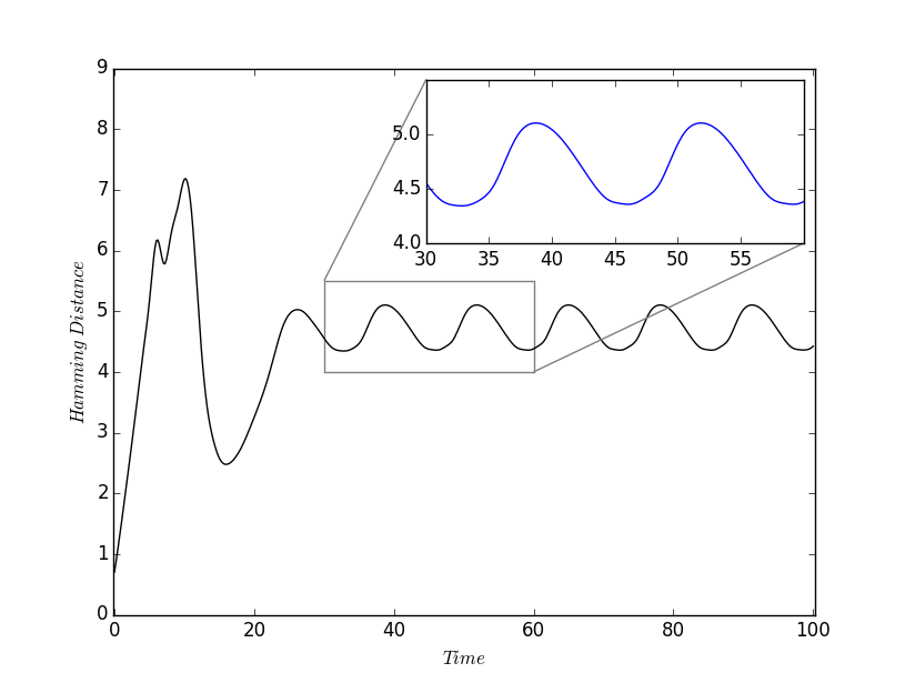
Figure 6: Hamming distance given by Eqn. 1 as a function of time, in a heterogeneous population comprising initially of a random mixture of individuals, with $S_{0}=R_{0}$ and $I_{0}=0.1$.

Another pertinent observation here is the dependence of this dynamics on disease cycle. As the length of the infectious stage (i.e. $\tau_{I}$) increases, keeping the total disease cycle length invariant, the fraction of infected individuals $I_{t}$ increases. The average $I_{t}$ is proportional to the fraction of the disease cycle occupied by the infectious stage, i.e the ratio $\tau_{I}/\tau_{0}$. So the size of the infected population strongly depends on the nature of disease as reflected in the length of the infectious stage of the disease.

III Influence of the initial composition of the population on the persistence of infection

We now attempt to gauge the statistically significant trends in $I_{t}$, by averaging the fraction of infected individuals at asymptotic time $t$, arising from a wide range of initial configurations at time $t=0$. We denote this by $\langle I_{t}\rangle$. In terms of this quantity, persistent infection is indicated by a non-zero value. However, after sufficient transient timesteps, if $\langle I_{t}\rangle$ is zero, it indicates that the infection has died out. So $\langle I_{t}\rangle$ can serve as an order parameter for the transition to sustained infection in a population.

III.1 Dependence of persistence of infection on the initial fraction of susceptibles

For fixed $\tau_{I}$ and $\tau_{0}$ we have calculated $\langle I_{t}\rangle$, for different initial fractions of susceptible individuals $S_{0}$. We explore the full possible range of $S_{0}\in[0,1]$, where $S_{0}=0$ signifies a population comprised entirely of refractory individuals who are immune to infection initially, and $S_{0}=1$ implies an initial population comprised entirely of individuals susceptible to infection. While the phase of the susceptible (S) sub-population is $\tau_{i,j}=0$ of course, the refractory individuals (R) can be present in different stages in the refractory period with $\tau_{I}<\tau_{i,j}<\tau_{0}$. We explore two different scenarios of the initial state of the refractory individuals in the population.

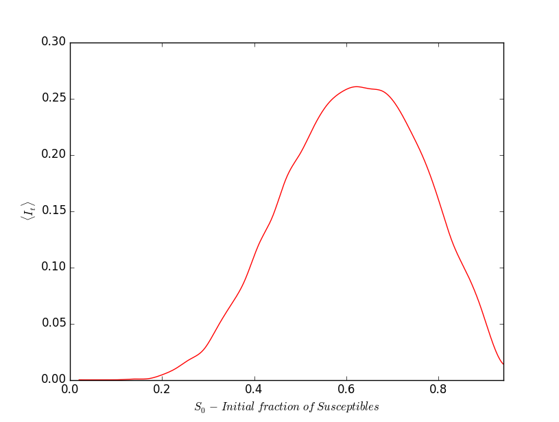
Figure 7: Variation of $\langle I_{t}\rangle$ (after transience) with respect to the fraction of susceptible individuals in the initial population $S_{0}$, arising from the presence of a single infected individual at time $t=0$. Here the refractory individuals have the same phase, the disease cycle has $\tau_{I}=4$; $\tau_{0}=13$, and $I_{t}$ is averaged over $10^{3}$ realizations of the initial population on the lattice. The specific case of a $100\times 100$ lattice is displayed. However note that different lattice sizes yield the same result.

First we present the case where all the refractory individuals are at the start of the refractory stage of the disease cycle, i.e. all $\tau_{i,j}=\tau_{I}+1$. So there is uniformity in the stage of disease progression in the refractory sub-population, though the individuals are randomly distributed spatially. We focus on the asymptotic state of infection in such a population, arising from a single infected individual at the outset. The results obtained from a large sample of initial states is shown in Fig. 7, and it is evident from there that $\langle I_{t}\rangle$ is very low for both high and low $S_{0}$, peaking around $S_{0}\sim 0.65-0.75$. Namely, homogeneous initial populations where all individuals are immune ($S_{0}=0$), or all are susceptible to disease ($S_{0}=1$), do not yield persistent infection. Rather, mixed populations lead to most sustained infection, with persistently high numbers of infected individuals.

We can rationalize our observations as follows: If an infected individual is completely surrounded by refractory individuals with $\tau=\tau_{I}+1$, it will complete the infectious stage without transferring the infection at all, as $\tau_{I}<\tau_{R}$. So the infection can spread only if the infected seed is contiguous to at least one susceptible individual. Now the probability of contact with a susceptible individual in the initial stages of infection spreading depends on the initial fraction of susceptibles $S_{0}$. This suggests that when $S_{0}$ is low, the chance of the infected individual being in contact with a susceptible one is low. As a result, as $S_{0}$ tends to zero, on an average, the infection eventually gets removed from the population, with the seed of infection crossing over to the refractory phase without infecting any other individual.

When there are more susceptible individuals in the initial population, there is a higher chance that the infected seed will encounter a susceptible neighbour. So as expected, increasing $S_{0}$ leads to a larger infected set on an average. However the surprising trend is the decrease in the infected set as the initial susceptible sub-population becomes too high, with the number of infected individuals tending to zero as the entire population becomes susceptible. This feels counter-intuitive, but can be understood as follows: Consider the limiting case where initially almost all the individuals are susceptible to the infection. Now the infection will spread immediately in isotropic waves, but will eventually stop at the boundaries. In analogy to the spread of forest fire, the boundary of refractory individuals is like scorched earth preventing spread across them. Now after the wave of infection passes, the individuals are in the refractory stage, leading eventually to the entire set being synchronized in the susceptible regime. There is no infected individual left then to act as a seed for a further wave of infection spreading. So the infection does not persist. The susceptible stage is like an “absorbing state”, and in the absence of “infectious perturbation” the system remains fixed in that state.

In order to prevent the above scenario, one needs enough refractory individuals in the population. When $R_{0}$ is below $1/4$ (i.e. $S_{0}>3/4$), typically the infected seed may not have a refractory individual among its four neighbours. So one expects that the persisting infection will have lower probability of occurrence as $S_{0}$ increases beyond $3/4$. This is in accordance with the trends observed in the simulations.

We then see that for the infection to persist in a population, a well mixed heterogeneous population is required, with reasonable number of both susceptible and refractory individuals. Randomly mixed populations prevent synchronization of the disease, and this is the key to always having some source of infection left in the population.

III.2 Dependence of persistence of infection on the initial fraction of infecteds

We now vary the initial fraction of infected individuals $I_{0}$ in the population, over the entire range $[0,1]$. For the remaining population, the initial fraction of susceptible and refractory individuals is set at different ratios. We consider an ensemble of initial conditions, with specific $I_{0}$, $S_{0}$ and $R_{0}$ and find the time averaged $I_{t}$, after long transience for each realization. The ensemble average of this quantity is displayed in Fig. 8. Notably, we find that there is a definite window of persistence over the range of $I_{0}$, where the infection never dies down and the fraction of infected individuals in the population is reasonably high on an average.

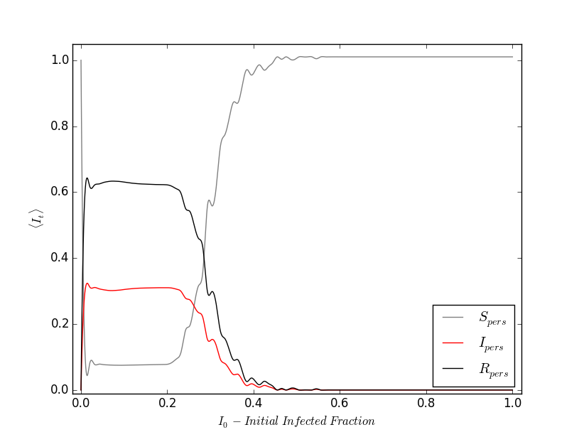
Figure 8: Variation of $\langle I_{t}\rangle$ (after transience) with respect to the initial fraction of infected individuals $I_{0}$ in the population, and $S_{0}=R_{0}$. The refractory sub-population consists of individuals with phase equal to $\tau_{I}+1$. Here the disease cycle has $\tau_{I}=4$; $\tau_{0}=13$, and $I_{t}$ is averaged over $10^{3}$ initial realizations. The specific case of a $100\times 100$ lattice is displayed. However note that different lattices sizes yield the same result.

In the state where infection is persistent, the individuals are unsynchronized and spread over the different stages of the disease cycle. So on an average the fraction of infected individuals is $\sim\tau_{I}/\tau_{0}$, namely the fraction of the total disease cycle occupied by the infected stage. For instance, in the example shown in Fig. 8 with $\tau_{I}=4$ and $\tau_{0}=13$, at the plateau of persistence, the infected fraction is approximately one-third of the population.

The transition to persistent infection is sharp and occurs at $I_{0}\rightarrow 0$. This implies that the infection can spread and persist even when there is only a single infected individual in the initial population. This is consistent with the results we presented earlier (cf. Fig. 7) on infection spreading from a single infected individual.

Interestingly, the infection ceases to persist for higher values of $I_{0}$, and the fall in persistence is rapid. That is, if the initial population has too many infected individuals, infection will not persist. This can be rationalized by noting that one needs a mix of susceptibles and refractory individuals in the population for persistent infection. For instance, considering the limiting case of all infected individuals in the initial state, it is clear that all individuals will go through the disease cycle in synchrony. So all individuals will become susceptible again together, but there will be no infective seed left in the population to perpetuate the infection.

IV Effect of varying degrees of non-uniformity in the refractory sub-population on the persistence of infection

Now we will explore the effect of non-uniformity within the refractory sub-population on the emergence of persistent infections. Namely, we will consider the refractory individuals in the initial population to be in different stages of disease progression. We will consider two distinct ways of interpolating between the completely heterogeneous and completely uniform limiting cases, in order to gauge the effect of heterogeneity on sustaining infection.

First we consider the initial refractory sub-population to be an admixture of subsets of individuals with uniform phase and with randomly distributed phases. Specifically, we explore initial refractory sub-populations comprised of some fraction $f_{rand}$ with phases randomly distributed over the range $\tau_{I}+1$ to $\tau_{0}$, and the rest $1-f_{rand}$ with fixed phase $\tau_{R}=\tau_{I}+1$. We examine the spread and persistence of infection in such a scenario, under variation of the initial composition of the population.

Fig 9 exhibits the persistence of infection, with respect to varying $S_{0}$, arising in a population that had a single infected individual initially. Different fractions of the initial refractory sub-population with randomized phases were explored, ranging from $f_{rand}=0$ (i.e. completely uniform), to $f_{rand}=1$ (i.e. completely heterogeneous). The trends clearly indicate a continuous cross-over from the condition where all refractory individuals are in the same phase, to the scenario where all are in random phases.

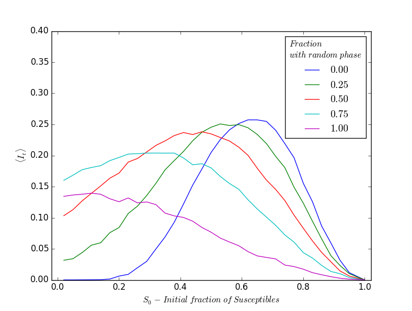
Figure 9: Variation of $\langle I_{t}\rangle$ (after transience) with respect to initial fraction of susceptible individuals $S_{0}$, for different fractions $f_{rand}$ of the initial refractory sub-population having randomly distributed phases (see key). Here the disease cycle has $\tau_{I}=4$; $\tau_{0}=13$, and $I_{t}$ is averaged over $10^{3}$ initial realizations and lattice size is $100\times 100$.

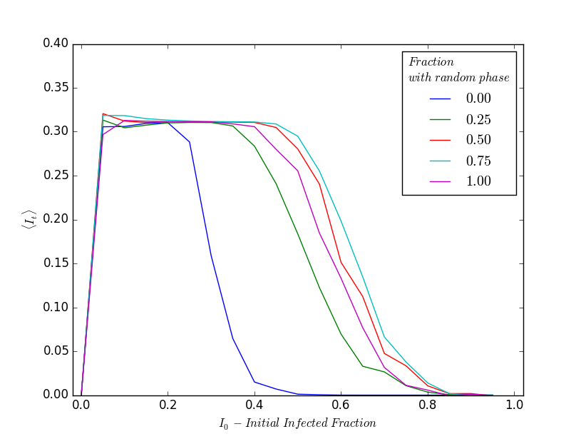
Figure 10: Variation of $\langle I_{t}\rangle$ (after transience) with respect to the initial fraction of infected individuals $I_{0}$ in the population, and $S_{0}=R_{0}$. The initial refractory sub-population consists of different fractions $f_{rand}$ with randomly distributed phases (see key). Here the disease cycle has $\tau_{I}=4$; $\tau_{0}=13$, and $I_{t}$ is averaged over $10^{3}$ initial realizations. While the specific case of a $100\times 100$ lattice is displayed, different lattices sizes yield the same result.

Further, we explore the effect of varying the initial fraction of infected individuals $I_{0}$, over the range $[0,1]$. Fig. 10 exhibits the change in the window of persistence with respect to $f_{rand}$. It is evident that increasing $f_{rand}$, namely increasing the initial number of refractory individuals with de-synchronized phases, leads to a definite increase in the window of persistence. This implies that for populations with a more heterogeneous refractory sub-population, the disease persists over a larger range of infected fractions $I_{0}$ of the initial population.

Note however, that there is also an apparent reduction in the window of persistence at very high $f_{rand}$. This can be rationalized by noting that when the entire initial refractory sub-population $R_{0}$ has uniformly distributed phases, there are a significant number of individuals who are closer to the end of their disease cycle (for instance, stage $12$ or $13$). These individuals become susceptible within a few time steps, and therefore bring the population closer to an overall state of homogeneity again, as all susceptibles are in the same phase (stage 0) and remain in that phase unless infected. We have observed qualitatively and quantitatively earlier, that a more homogeneous population leads to a reduced window of persistence. Hence, presence of a significant number of individuals closer to the end of their disease cycle acts as a homogenizing factor for the population and is detrimental to persistence.

Lastly, we study the effect of varying ranges of spread in the initial phases of the refractory individuals. Specifically we consider that the phase of the refractory individuals in the initial population to be randomly distributed over different ranges $R_{rand}$. In particular we examine the persistence of infection for $R_{rand}$ ranging from $[\tau_{I}+1,\tau_{I}+1]$, (where all refractory individuals have the same phase) to [$\tau_{I}+1$, $\tau_{I}+\tau_{R}$] (where heterogeneity is large as the phases of the refractory individuals are distributed over the entire refractory range).

Fig. 12 exhibits representative results of $\langle I_{t}\rangle$ as a function of the initial fraction of susceptibles $S_{0}$, for the case where there is a single infected individual in the population at the outset. It can be clearly seen that a smooth cross-over takes place from the extremal case of all refractory individuals in the same phase, to the limit where the stages of the refractory individuals are spread randomly over the entire refractory period. The key observation here is that as the spread in phases increases, the range of persistent infection becomes larger. Namely, when there is a large initial spread in the stages of disease among the individuals, at subsequent times there are always some individuals who can “pick up the baton of infection”, leading to persistent infection.

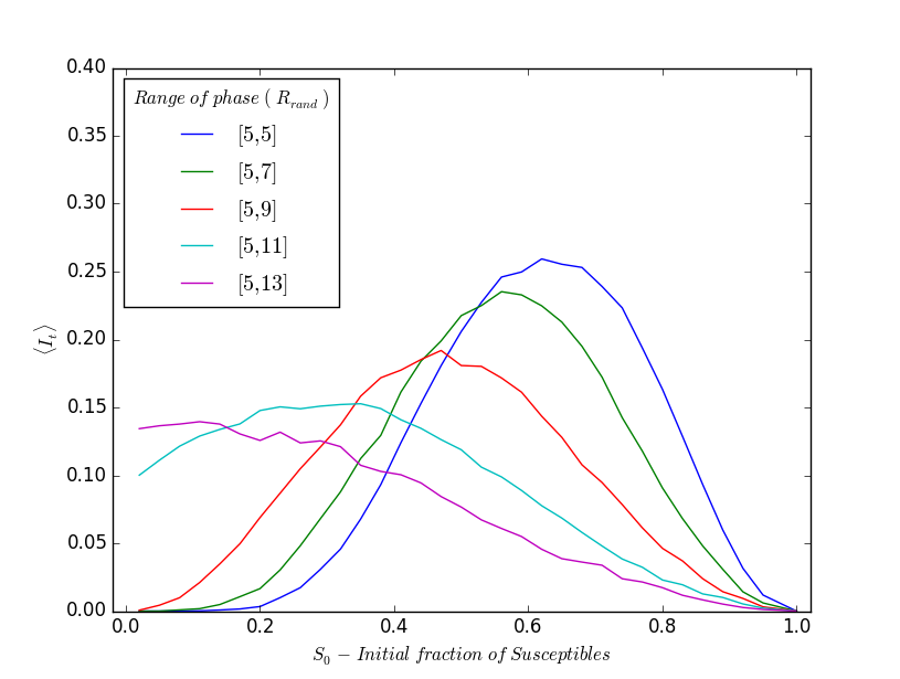
Figure 11: Variation of $\langle I_{t}\rangle$ (after transience) with respect to initial fraction of susceptible individuals $S_{0}$, for the refractory individuals having phases $\tau$ randomly distributed over different ranges $R_{rand}$ in the refractory stage : [5,5]; [5,7]; [5,9]; [5,11]; [5,13]. Here $I_{t}$ is averaged over $10^{3}$ realizations, lattice size is $100\times 100$, and the disease cycle parameters $\tau_{I}=4$, $\tau_{0}=13$.

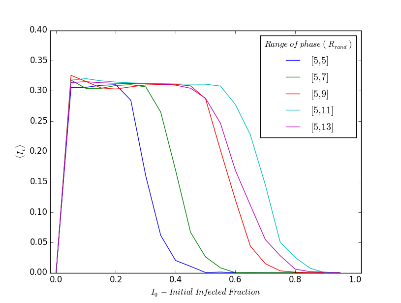
Figure 12: Variation of $\langle I_{t}\rangle$ (after transience) with respect to initial fraction of infected individuals $I_{0}$, for the refractory individuals having phases $\tau$ randomly distributed over different ranges $R_{rand}$ in the refractory stage : [5,5]; [5,7]; [5,9]; [5,11]; [5,13]. Here $I_{t}$ is averaged over $10^{3}$ realizations, lattice size is $100\times 100$, and the disease cycle parameters $\tau_{I}=4$, $\tau_{0}=13$.

So we see that in the completely heterogeneous case, low susceptible and high refractory initial subpopulations favour persistent infection. But in a completely uniform population, a higher fraction of susceptibles leads to persistent infection. This has the following important implication: when refractory individuals are not synchronized at the same phase of disease progression, even if there are few susceptible individuals in the population initially, the infection grows substantially and the average size of the infected sub-population is large. So we have demonstrated that even when the entire population is susceptible to infection, the infection eventually dies out, while even a few susceptibles among an heterogeneous refractory population gives rise to a large persistent infected sub-population.

We can rationalize this counter-intuitive trend that persistent infection is more likely when the number of susceptible individuals in the initial population is low, as follows: When $S_{0}$ is low, there are many refractory individuals in the population surrounding the infected individual. These individuals are in various stages in the refractory period, and some become susceptible again while the seed is still infectious. If $S_{0}\rightarrow 0$ and the refractory individuals are uniformly distributed over the refractory range $\tau_{R}$, the probability of the seed encountering a susceptible individual while still infectious is proportional to $\tau_{I}/\tau_{R}$. Since at least one neighbour in contact with the seed needs to be susceptible, this probability should be greater than $\frac{1}{4}$ for the infection to spread, on an average. So when the infective stage $\tau_{I}$ is sufficiently long (as in our example of $\tau_{I}=4$, in a disease cycle of length $13$), extremely low initial $S_{0}$ can also lead to persistent infection.

V Conclusion

In summary, we have explored the emergence of persistent infection in a patch of population, where the disease progression of the individuals was given by the SIRS model and an individual became infected on contact with another infected individual. We investigated the infection spreading qualitatively and quantitatively, under varying degrees of heterogeneity in the initial population.

Specifically, we considered two scenarios extrapolating between the completely homogeneous and completely heterogeneous limit. One considers varying fractions of heterogeneous sub-populations and another examines varying ranges in the spread of the stages of disease progression. Our central result is the following: we find that an infectious seed does not give rise to persistent infection in a homogeneous population consisting of individuals at the same stage of disease progression. Rather, when the population is heterogeneous, and consists of randomly distributed individuals at various stages of the disease, infection becomes persistent in the population patch. The key to persistent infection is then the random admixture of refractory and susceptible individuals, leading to de-synchronization of the phases in the disease cycle of the individuals. So we have demonstrated that when the entire population is susceptible to infection, the infection eventually dies out, while even a few susceptibles among an heterogeneous refractory population gives rise to a large persistent infected sub-population.

Author contributions

SS conceived the problem, and VA and PM performed all the numerical simulations. SS, VA and PM discussed the results and wrote the manuscript together.

The authors declare no competing financial interests.

References

- (1) C. McEvedy, Sci. Am., 258 (1988) 74
- (2) M.M. Kaplan and R.G. Webster, Sci. Am., 237 (1977) 88
- (3) A. Cliff and P. Haggett, Sci. Am., 250 (1984) 110
- (4) J.D. Murray, Mathematical Biology (Springer-Verlag, Berlin, 1993).
- (5) L. Edelstein-Keshet, Mathematical Models in Biology (Random House, New York, 1988).
- (6) E.M.Rauch, H. Sayama and Y. Bar-Yam, J. theor. Biol., 221 (2003) 655
- (7) C. Moore, M.E.J. Newman, Phys. Rev. E, 61 (2000), 5678
- (8) R.M. May, A.L. Lloyd, Phys. Rev. E, 64 (2001), 066112
- (9) R. Pastor-Satorras, A. Vespignani, Phys. Rev. E, 63 (2001), 066117
- (10) H.W. Hethcote Math Bioscience 28 (1976) 335.
- (11) C. Ozcaglar, A. Shabbeer, S.L. Vandenberg, B. Yener, and K.P. Bennett, Math Biosci., 236 (2012) 77–96.
- (12) M. Kuperman and G. Abramson, Phys. Rev. Letts., 86 (2001) 2909
- (13) P.M. Gade and S. Sinha, Phys Rev E, 72 (2005) 052903.
- (14) V. Kohar and S. Sinha, Chaos, Solitons Fractals, 54 (2013) 127-134.
- (15) C.J. Rhodes and R.M. Anderson, Phys. Letts. A, 210 (1996) 183-188.