Computation of highly oscillatory Bessel transforms with algebraic singularities

Abstract

In this paper, we consider the Clenshaw-Curtis-Filon method for the highly oscillatory Bessel transform $\int_{0}^{1}x^{\alpha}(1-x)^{\beta}f(x)J_{\nu}(\omega x)dx$, where $f$ is a smooth function on $[0,1]$, and $\nu\geq 0.$ The method is based on Fast Fourier Transform (FFT) and fast computation of the modified moments. We give a recurrence relation for the modified moments and present an efficient method for the evaluation of modified moments by using recurrence relation. Moreover, the corresponding error bound in inverse powers of $N$ for this method for the integral is presented. Numerical examples are provided to support our analysis and show the efficiency and accuracy of the method.

1 Introduction

The fast computation of highly oscillatory Bessel transforms

$$I[f]=\int_{0}^{1}x^{\alpha}(1-x)^{\beta}f(x)J_{\nu}(\omega x)dx,\quad\nu\geq 0$$ (1.1)

where $\alpha>-1,\beta>-1$, and $f$ is a sufficiently smooth function on $[0,1]$, $J_{\nu}(x)$ is the Bessel function of the first kind and order $\nu$, plays an important role in many areas of science and engineering, such as astronomy, optics, quantum mechanics, seismology image processing, electromagnetic scattering (for example [2], [3], [10], [17]). In most of the cases, the oscillatory integrals with Bessel kernels can not be evaluated analytically and one has to resort to numerical methods. Particularly, for large $\omega$, the integrands become highly oscillatory. Hence, it presents serious difficulties in approximating the integral by classical numerical methods like Simpson rule, Gaussian quadrature, etc.

In recent years, there has been tremendous interest in developing numerical methods for the integral $\int_{a}^{b}f(x)J_{\nu}(\omega x)dx$, such as Levin method [19, 20], Levin-type method [23], modified Clenshaw-Curtis method [24], generalized quadrature rule [12, 13], Filon-type method [29], Gauss-Laguerre quadrature[5, 6]. To avoid the Runge phenomenon, a Clenshaw-Curtis-Filon-type method was presented in [30]. Since, the integrand in (1.1) may have singularities at two end points, these methods cannot be applied to evaluating the integral (1.1) directly. Recently, a Filon-type method based on a special Hermite interpolation polynomial at Clenshaw-Curtis points was introduced in [7]. The key issue is the computation of modified moments. However, the algorithm [7] to evaluate the modified moments by transferring the Chebyshev interpolation polynomial into power series of $x^{k}$ is quite unstable for the number of nodes $N\geq 32$.

In this paper, we are concerned with the Clenshaw-Curtis-Filon method for the computation of the highly oscillatory Bessel transform (1.1) based on fast computation of modified moments. Moreover, this method can be applied to the Filon-type method based on Clenshaw-Curtis points given in [7].

This paper is organized as follows. In Section 2, we describe the Clenshaw-Curtis-Filon method for the integral (1.1). Meanwhile, we deduce a recurrence relation for the modified moments, and present an efficient algorithm for the moments. Error analysis about $N$ for the presented method for the integral (1.1) is derived in Section 3. We show that the method converges uniformly in $N$ for fixed $\omega$. In Section 4, several numerical examples are given to illustrate the accuracy and efficiency of the presented method.

2 Clenshaw-Curtis-Filon method for the integral (1.1)

Polynomial interpolation is used as one of the basic means of approximation in most areas of numerical analysis. To avoid Runge phenomenon, we consider a special Lagrange interpolation polynomial at the Clenshaw-Curtis points, instead of equally spaced points. Suppose that $f$ is absolutely continuous on $[0,1]$, and let $P_{N}(x)$ be the interpolant of $f$ at the Clenshaw-Curtis points

$$c_{i}=\frac{1}{2}+\frac{1}{2}\cos\left(\frac{i\pi}{N}\right),\textrm{\qquad}i=0,1,\ldots,N,$$

defined by $P_{N}(x)=\sum_{i=0}^{N}b_{i}T_{i}^{\ast}(x)$, where $T_{i}^{*}(x)$ denotes the shifted Chebyshev polynomial of the first kind on $[0,1]$, and the coefficients $b_{i}$ can be evaluated by FFT [8, 9, 26, 27]. The Clenshaw-Curtis-Filon method (CCF) for (1.1) is defined by

$$Q^{CCF}[f]=\int_{0}^{1}P_{N}(x)x^{\alpha}(1-x)^{\beta}J_{\nu}(\omega x)dx=\sum_{k=0}^{N}b_{k}M(k,\nu,\omega),$$ (2.1)

where

$$M(k,\nu,\omega)=\int_{0}^{1}x^{\alpha}(1-x)^{\beta}T_{k}^{\ast}(x)J_{\nu}(\omega x)dx,$$ (2.2)

denote the modified moments.

2.1 A recurrence relation for $M(k,\nu,\omega)$

In the following, we present a recurrence relation for the modified moments $M(k,\nu,\omega)$.

Theorem 2.1

The sequence $M(k,\nu,\omega),k\geq 4$ satisfies the following recurrence relation:

$$\frac{\omega^{2}}{16}M(k+4,\nu,\omega)+\Big{[}(k+3)^{2}-{\nu}^{2}-\frac{\omega^{2}}{4}+(\alpha+\beta)^{2}+(6+2k)(\alpha+\beta)\Big{]}M(k+2,\nu,\omega)$$ (2.3)

$$+ \Big{[}(4{\nu}^{2}+2k+4)-4(\alpha^{2}-\beta^{2})-4k(\alpha-\beta)-8\alpha+12\beta\Big{]}M(k+1,\nu,\omega)$$

$$+ \Big{[}6(\alpha^{2}+\beta^{2})+(4\alpha+12\beta-4\alpha\beta)-2k^{2}+6-6{\nu^{2}}+\frac{3\omega^{2}}{8}\Big{]}M({k},\nu,\omega)$$

$$+ \Big{[}(4{\nu}^{2}-2k+4)-4(\alpha^{2}-\beta^{2})-4k(\alpha-\beta)-8\alpha+12\beta\Big{]}M(k-1,\nu,\omega)$$

$$+ \Big{[}(k-3)^{2}-{\nu}^{2}-\frac{\omega^{2}}{4}+(\alpha+\beta)^{2}+(6-2k)(\alpha+\beta)\Big{]}M(k-2,\nu,\omega)$$

$$+ \frac{\omega^{2}}{16}M(k-4,\nu,\omega)=0.$$

Proof: Firstly, we rewrite the modified moments as

$$M(k,\nu,\omega)=\frac{1}{2^{\alpha+\beta+1}}\int_{-1}^{1}(1+x)^{\alpha}(1-x)^{\beta}T_{k}(x)J_{\nu}\Big{(}\frac{1+x}{2}\omega\Big{)}dx,$$ (2.4)

where $T_{k}(x)$ is the Chebyshev polynomial of degree $k$.

Let

$$K_{1}=4\int_{-1}^{1}(1+x)^{\alpha}(1-x)^{\beta}(1-x)^{2}(1+x)^{2}T_{k}(x)\bigg{[}J_{\nu}\Big{(}\frac{1+x}{2}\omega\Big{)}\bigg{]}^{\prime\prime}dx,$$ (2.5)

$$K_{2}=4\int_{-1}^{1}(1+x)^{\alpha}(1-x)^{\beta}(1-x)^{2}(1+x)T_{k}(x)\bigg{[}J_{\nu}\Big{(}\frac{1+x}{2}\omega\Big{)}\bigg{]}^{\prime}dx,$$ (2.6)

and

$$K_{3}=4\int_{-1}^{1}(1+x)^{\alpha}(1-x)^{\beta}(1-x)^{2}\Big{(}\nu^{2}-\frac{(1+x)^{2}\omega^{2}}{4}\Big{)}T_{k}(x)J_{\nu}\Big{(}\frac{1+x}{2}\omega\Big{)}dx.$$ (2.7)

According to the fact that [1]

$$x^{2}\frac{d^{2}J_{\nu}(x)}{dx^{2}}+x\frac{dJ_{\nu}(x)}{dx}+(x^{2}-\nu^{2})J_{\nu}(x)=0,$$ (2.8)

we can easily obtain the equality

$$K_{1}+K_{2}-K_{3}=0.$$ (2.9)

Using the identity that [21]

$$x^{m}T_{n}(x)=2^{-m}\sum_{j=0}^{m}\binom{m}{j}T_{n+m-2j}(x)$$

and integration by parts, we have

$$K_{1}= \Big{[}(\alpha^{2}+\beta^{2}+k^{2})+2(\alpha\beta+\alpha k+\beta k)+7(\alpha+\beta+k)+12\Big{]}M(k+2,\nu,\omega)$$ (2.10)

$$+\Big{[}4(\beta^{2}-\alpha^{2})+(4k+12)(\beta-\alpha)\Big{]}M(k+1,\nu,\omega)$$

$$+\Big{[}6(\alpha^{2}+\beta^{2})+10(\alpha+\beta)-4\alpha\beta-2k^{2}+8\Big{]}M(k,\nu,\omega)$$

$$+\Big{[}4(\beta^{2}-\alpha^{2})+(12-4k)(\beta-\alpha)\Big{]}M(k-1,\nu,\omega)$$

$$+\Big{[}(\alpha^{2}+\beta^{2}+k^{2})+2(\alpha\beta-\alpha k-\beta k)+7(\alpha+\beta-k)+12\Big{]}M(k-2,\nu,\omega),$$

$$K_{2}= -\Big{\{}(\alpha+\beta+k+3)M(k+2,\nu,\omega)-(4+4\alpha+2k)M(k+1,\nu,\omega)+(6\alpha-2\beta+2)$$ (2.11)

$$M(k,\nu,\omega)-(4+4\alpha-2k)M(k-1,\nu,\omega)+(\alpha+\beta-k+3)M(k-2,\nu,\omega)\Big{\}},$$

and

$$K_{3}= -\frac{1}{16}\bigg{\{}\omega^{2}M(k+4,\nu,\omega)-(4\omega^{2}+16\nu^{2})M(k+2,\nu,\omega)+64\nu^{2}M(k+1,\nu,\omega)+$$ (2.12)

$$(6\omega^{2}-96\nu^{2})M(k,\nu,\omega)+64\nu^{2}M(k-1,\nu,\omega)-(4\omega^{2}+16\nu^{2})M(k-2,\nu,\omega)$$

$$+\omega^{2}M(k-4,\nu,\omega)\bigg{\}}.$$

A combination of (2.9)-(2.12) gives the desired result.  

2.2 Fast computations of the modified moments

Now, we turn to the fast computations of the modified moments via recurrence relation (2.3). Because of the symmetry of the recurrence relation of the Chebyshev polynomials $T_{j}(x)$, it is convenient to define $T_{-j}(x)=T_{j}(x),j=1,2,\ldots$, then it holds that $M(-j,\nu,\omega)=M(j,\nu,\omega)$. It can be shown that (2.3) is not only valid for $k\geq 4$, but also for all integers of $k$. However, both forward and backward recursion are asymptotically unstable [24]. Fortunately, the instability is less pronounced if $\omega$ is large, and practical experiments show that the modified moments $M(j,\nu,\omega)$ can be computed accurately using forward recursion if $k\leq\omega/2$. For the case $k\geq\frac{\omega}{2}$, forward recursion is no longer feasible, since the loss of significant figures increases. In this case, the moments can be computed by Oliver’s algorithm [22] with six starting moments and two end moments. The end moments can be approximated by converting $M(k,\nu,\omega)$ into the form of Fourier integral and using asymptotic expansion in [11].

Using the explicit expression of the shifted Chebyshev polynomials [21]

$$T_{k}^{\ast}(x)=T_{2k}(\sqrt{x})=\sum_{j=0}^{k}c_{j}^{(2k)}x^{k-j},$$

where

$$c_{j}^{(2k)}={(-1)}^{j}2^{2k-2j-1}\Big{[}2\binom{2k-j}{j}-\binom{2k-j-1}{j}\Big{]},$$

the first few modified moments can be evaluated efficiently as follows:

$$M(k,\nu,\omega)=\sum_{j=0}^{k}c_{j}^{(2k)}I(\alpha+k-j,\beta,\nu,\omega),$$ (2.13)

and $I(\alpha+k-j,\beta,\nu,\omega)=\int_{0}^{1}x^{\alpha+k-j}(1-x)^{\beta}J_{\nu}(\omega x)dx$ can be computed by the formula [15, p. 681]

$$\int_{0}^{1}x^{a}(1-x)^{b}J_{\nu}(\omega x)dx$$ (2.14)

$$= \frac{\Gamma(b+1)\Gamma(a+\nu+1)\leftidx{{}_{2}}{F}{{}_{3}}(\frac{a+\nu+1}{2},\frac{a+\nu+2}{2};\nu+1,\frac{a+b+\nu+2}{2},\frac{a+b+\nu+3}{2};-\frac{\omega^{2}}{4})}{2^{\nu}\omega^{-\nu}\Gamma(\nu+1)\Gamma(a+b+\nu+2)},$$

where $\Re(a+\nu)>-1,\Re(b)>-1$, and $\leftidx{{}_{2}}{F}{{}_{3}}(\mu_{1},\mu_{2};\nu_{1},\nu_{2},\nu_{3};z)$ denotes a class of generalized hypergeometric function.

Remark 1

Since $Y_{\nu}(x)$ and $J_{\nu}(x)$ are the solutions of the same differential equation, the integrals $\int_{0}^{1}x^{\alpha}(1-x)^{\beta}T_{k}^{\ast}(x)Y_{\nu}(\omega x)dx,k=0,1,\ldots,$ also satisfy the same recurrence relation (2.3). Moreover, the function $Y_{\nu}(x)$ can be expressed by the equation [4, p. 219]

$$Y_{\nu}(x)=G^{2,0}_{1,3}\left(\begin{array}[]{c}-\frac{\nu}{2}-\frac{1}{2}\\ -\frac{\nu}{2},\frac{\nu}{2},-\frac{\nu}{2}-\frac{1}{2}\end{array}\Bigg{|}\frac{x^{2}}{4}\right).$$ (2.17)

According to the identity that [16]

$$\int_{0}^{x}t^{\alpha-1}(x-t)^{\beta-1}G^{m,n}_{p,q}\left(\begin{array}[]{c}a_{1}\ldots a_{n},a_{n+1}\ldots a_{p}\\ b_{1}\ldots b_{m},b_{m+1}\ldots b_{q}\end{array}\Bigg{|}\omega t^{l}\right)dt$$ (2.20)

$$= \frac{l^{-\beta}\Gamma(\beta)}{x^{1-\alpha-\beta}}G^{m,n+l}_{p+l,q+l}\left(\begin{array}[]{c}\frac{1-\alpha}{l},\ldots,\frac{l-\alpha}{l},a_{1}\ldots a_{n},a_{n+1}\ldots a_{p}\\ b_{1}\ldots b_{m},b_{m+1}\ldots b_{q},\frac{1-\alpha-\beta}{l},\ldots,\frac{l-\alpha-\beta}{l}\end{array}\Bigg{|}\omega x^{l}\right),$$ (2.23)

the first several starting values of the modified moments $\int_{0}^{1}x^{\alpha}(1-x)^{\beta}T_{k}^{\ast}(x)Y_{\nu}(\omega x)dx,k=1,2,\ldots$ can be evaluated by the following formula

$$\int_{0}^{1}x^{a}(1-x)^{b}Y_{\nu}(\omega x)dx=\frac{\Gamma(b+1)}{2^{b+1}}G^{2,2}_{3,5}\left(\begin{array}[]{c}-\frac{a}{2},\frac{1-a}{2},-\frac{\nu}{2}-\frac{1}{2}\\ -\frac{\nu}{2},\frac{\nu}{2},-\frac{\nu}{2}-\frac{1}{2},-\frac{a+b+1}{2},-\frac{a+b}{2}\end{array}\Bigg{|}\frac{1}{4}\omega^{2}\right)$$ (2.26)

by a similar way to the modified moments $M(k,\nu,\omega)$. As this idea is tangential to the topic of this paper, we will not study it further.

3 Error analysis and uniform convergence for the Clenshaw-Curtis-Filon method

In practical problems the frequency $\omega$ is always fixed. To guarantee the convergence of the method for the fixed $\omega$ with respect to the number of quadrature nodes, we mainly focus on the error bound about $N$ for fixed $\omega$ in this section. We first introduce some lemmas.

Lemma 3.1

([11]) If $0<\lambda,\mu\leq 1$, and $\phi(t)$ is $N$ times differentiable for $a\leq t\leq b$, then

$$\int_{a}^{b}(t-a)^{\lambda-1}(b-t)^{\mu-1}e^{irt}\phi(t)dt=B_{N}(r)-A_{N}(r)+O(r^{-N}),$$ (3.1)

where

$$A_{N}(r) =\sum_{n=0}^{N-1}\frac{\Gamma({n+\lambda})}{n!}e^{i\pi(n+\lambda-2)/2}\omega^{-n-\lambda}e^{ira}\bigg{[}\frac{d^{n}}{dt^{n}}\big{\{}(b-t)^{\mu-1}\phi(t)\big{\}}\bigg{]}_{t=a},$$

$$B_{N}(r) =\sum_{n=0}^{N-1}\frac{\Gamma({n+\mu})}{n!}e^{i\pi(n-\mu)/2}\omega^{-n-\mu}e^{irb}\bigg{[}\frac{d^{n}}{dt^{n}}\big{\{}(t-a)^{\lambda-1}\phi(t)\big{\}}\bigg{]}_{t=b}.$$

Lemma 3.2

Suppose that $f\in C^{\kappa+1}[a,b]$, for each $\alpha>-1,\beta>-1$, and $r\gg 1$, it holds that

$$\int_{a}^{b}(x-a)^{\alpha}(b-x)^{\beta}f(x)e^{irx}dx=O\Big{(}r^{-1-\min\big{\{}\alpha,\beta\big{\}}}\Big{)},$$ (3.2)

where $\kappa=\Big{\lceil}\min\big{\{}\alpha,\beta\big{\}}\Big{\rceil}$, and $\big{\lceil}z\big{\rceil}$ denotes the smallest integer not less than $z$.

Proof: We only prove (3.2) for the case $\alpha\leq\beta$, and the similar proof can be applied to the case $\alpha>\beta$.

Assume that $\alpha=\lceil\alpha\rceil+k_{1}=N_{1}+k_{1}$ and $\beta=\lceil\beta\rceil+k_{2}=N_{2}+k_{2}$, we have $N_{1}\leq N_{2}$ and $-1<k_{1},k_{2}\leq 0$. Then, it holds that

$$\int_{a}^{b}(x-a)^{\alpha}(b-x)^{\beta}f(x)e^{irx}dx$$ (3.3)

$$= \int_{a}^{b}e^{irx}(x-a)^{k_{1}}(b-x)^{k_{2}}(x-a)^{N_{1}}(b-x)^{N_{2}}f(x)dx$$

$$= \int_{a}^{b}e^{irx}(x-a)^{k_{1}}(b-x)^{k_{2}}F(x)dx,$$

where $F(x)=(x-a)^{N_{1}}(b-x)^{N_{2}}f(x)$.

If $N_{1}=0$, it yields the desired result by applying the Lemma 3.2 to the first identity of equation (3.3) directly.

If $N_{1}\geq 1$, it can be shown that

$$\bigg{[}\frac{d^{j}}{dx^{j}}\big{\{}(b-x)^{k_{2}}F(x)\big{\}}\bigg{]}_{x=a}=0,\quad j=0,\ldots,N_{1}-1,$$ (3.4)

and

$$\bigg{[}\frac{d^{j}}{dx^{j}}\big{\{}(x-a)^{k_{1}}F(x)\big{\}}\bigg{]}_{x=b}=0,\quad j=0,\ldots,N_{2}-1.$$ (3.5)

According to Lemma 3.1, a combination of (3.3)-(3.5) yields that

$$\int_{a}^{b}(x-a)^{\alpha}(b-x)^{\beta}f(x)e^{irx}dx=O\Big{(}r^{-N_{1}-k_{1}-1}\Big{)}=O\Big{(}r^{-1-\min\big{\{}\alpha,\beta\big{\}}}\Big{)}.$$

This completes the proof.  

Lemma 3.3

For each $j\geq 1,\alpha>-1,\beta>-1$ and fixed $\omega$, it is true that

$$\int_{0}^{1}x^{\alpha}(1-x)^{\beta}T_{j}^{\ast}(x)J_{\nu}(\omega x)dx=\left\{\begin{aligned} &O(j^{-2}),~{}~{}~{}~{}~{}~{}~{}~{}~{}~{}~{}~{}~{}~{}~{}~{}~{}~{}\alpha=\beta=-\frac{1}{2},\\ &O\Big{(}j^{-\min\big{\{}2,2+2\alpha\big{\}}}\Big{)},\quad\beta=-\frac{1}{2},\alpha>-\frac{1}{2},\\ &O\Big{(}j^{-\min\big{\{}2,2+2\beta\big{\}}}\Big{)},\quad\alpha=-\frac{1}{2},\beta>-\frac{1}{2},\\ &O\Big{(}j^{-2-2\min\big{\{}\alpha,\beta\big{\}}}\Big{)},\quad\mbox{otherwise}.\end{aligned}\right.$$ (3.6)

Proof: By changing the variables $x=\frac{1+t}{2}$ and $t=\cos(\theta)$, it yields that

$$\int_{0}^{1}x^{\alpha}(1-x)^{\beta}T_{j}^{\ast}J_{\nu}(\omega x)dx =\frac{1}{2}\int_{0}^{\pi}\sin(\theta)\cos^{2\alpha}(\theta/2)\sin^{2\beta}(\theta/2)\cos(j\theta)J_{\nu}(\omega\cos^{2}(\theta/2))d\theta$$ (3.7)

$$=2(-1)^{j}\int_{0}^{\frac{\pi}{2}}\sin^{2\alpha+1}(\theta)\cos^{2\beta+1}(\theta)\cos(2j\theta)J_{\nu}(\omega\sin^{2}(\theta))d\theta$$

$$=\frac{(-1)^{j}}{j}\int_{0}^{\frac{\pi}{2}}\sin^{2\alpha+1}(\theta)\cos^{2\beta+1}(\theta)J_{\nu}(\omega\sin^{2}(\theta))d\sin(2j\theta).$$

For the case $\alpha=\beta=-\frac{1}{2}$, we easily derive the first identity in (3.6) by integrating (3.7) by parts two times.

For the case $\beta=-\frac{1}{2},\alpha>-\frac{1}{2}$ or $\alpha=-\frac{1}{2},\beta>-\frac{1}{2}$, we rewrite the integral (3.7) as

$$\int_{0}^{1}x^{\alpha}(1-x)^{\beta}T_{j}^{\ast}(x)J_{\nu}(\omega x)dx$$ (3.8)

$$= 2(-1)^{j}\int_{0}^{\frac{\pi}{2}}\theta^{2\alpha+1}(\pi/2-\theta)^{2\beta+1}\Big{(}\frac{\sin(\theta)}{\theta}\Big{)}^{2\alpha+1}\Big{(}\frac{\cos(\theta)}{\pi/2-\theta}\Big{)}^{2\beta+1}J_{\nu}(\omega\sin^{2}(\theta))\cos(2j\theta)d\theta.$$

By using integration by parts one time for the integral (3.8) and Lemma 3.2, we can easily get the the second and third identities in (3.6).

For other cases, the fourth identity in (3.6) can be obtained by applying the Lemma 3.2 to integral (3.8) directly.  

Theorem 3.1

Suppose that $f(x)$ has an absolutely continuous $(k-1)$st derivative $f^{(k-1)}$ on $[0,1]$ and a $k$th derivative $f^{(k)}$ of bounded variation $V_{k}$ for some $k\geq 1$. Then, for each $\alpha>-1,\beta>-1,N\geq k+1$ and fixed $\omega$, the error bound about $N$ for the Clenshaw-Curtis-Filon method for the integral (1.1) satisfies

$$I[f]-Q^{CCF}[f]=\left\{\begin{aligned} &O\Big{(}N^{-2\min\big{\{}\alpha,\beta\big{\}}-k-2}\Big{)},\quad-1<\min\Big{\{}\alpha,\beta\Big{\}}<-\frac{1}{2},\\ &O\big{(}N^{-k-1}\big{)},~{}~{}~{}~{}~{}~{}~{}~{}~{}~{}~{}~{}~{}~{}~{}~{}~{}~{}\min\Big{\{}\alpha,\beta\Big{\}}\geq-\frac{1}{2}.\end{aligned}\right.$$ (3.9)

Proof: According to the ideas of [31, 32], the Chebyshev series for the function $f(x)$ can be expressed as [25, pp. 165]

$$f(x)=\sum^{\infty}_{j=0}{{}^{\prime}}a_{j}T^{\ast}_{j}(x),\quad a_{j}=\frac{\pi}{2}\int_{-1}^{1}\frac{f(\frac{1+x}{2})T_{j}(x)}{\sqrt{1-x^{2}}}dx,$$ (3.10)

where the prime indicates that the term with $j=0$ is multiplied by $1/2$. Also, the coefficients $a_{j}$ satisfy [26, 27]

$$|a_{j}|\leq\frac{2V_{k}}{\pi j(j-1)\cdot\cdot\cdot(j-k)}.$$ (3.11)

For each $j=0,1,\ldots,N$, $p=1,2,\ldots$, from the property of Chebyshev polynomials [14, p. 67], we can easily get the aliasing errors for the integration on Chebyshev polynomials

$$P_{N}(T^{\ast}_{pN+j})=\left\{\begin{aligned} &T^{\ast}_{N-j},\quad\mbox{if \emph{p} is odd},\\ &T^{\ast}_{j},~{}~{}~{}~{}~{}~{}~{}\mbox{if \emph{p} is even},\end{aligned}\right.$$ (3.12)

and

$$Q^{CCF}[T^{\ast}_{pN+j}]=\left\{\begin{aligned} &I[T^{\ast}_{N-j}],\quad\mbox{if \emph{p} is odd},\\ &I[T^{\ast}_{j}],~{}~{}~{}~{}~{}~{}~{}\mbox{if \emph{p} is even}.\end{aligned}\right.$$ (3.13)

For the case $\min\big{\{}\alpha,\beta\big{\}}\geq-1/2$, according to Lemma 3.3, there exists two constants $C$ and $\sigma>-1/2$ such that $|I[T^{\ast}_{j}]|\leq Cj^{-2-2\sigma}$. Thus, we have the following estimate:

$$|I[f]-Q^{CCF}[f]|$$ (3.14)

$$\leq \sum_{m=N+1}^{\infty}|a_{m}||I[T^{\ast}_{m}]-Q^{CCF}[T^{\ast}_{m}]|$$

$$= \sum_{p=1}^{\infty}\sum_{j=1}^{N}\Big{(}|a_{2pN+j}||I[T^{\ast}_{2pN+j}]-I[T^{\ast}_{j}]|+|a_{(2p-1)N+j}||I[T^{\ast}_{(2p-1)N+j}]-I[T^{\ast}_{N-j}]|\Big{)}$$

$$\leq \sum_{p=1}^{\infty}\sum_{j=1}^{N}\Bigg{(}\frac{2V_{k}\Big{(}\frac{C}{(2pN+j)^{2+2\sigma}}+\frac{C}{j^{2+2\sigma}}\Big{)}}{\pi(2pN+j)(2pN+j-1)\cdot\cdot\cdot(2pN+j-k)}$$

$$+\frac{2V_{k}\Big{(}\frac{C}{((2p-1)N+j)^{2+2\sigma}}+\frac{C}{(N-j)^{2+2\sigma}}\Big{)}}{\pi((2p-1)N+j)((2p-1)N+j-1)\cdot\cdot\cdot((2p-1)N+j-k)}\Bigg{)}$$

$$< \frac{2CV_{k}}{\pi N(N-1)\cdot\cdot\cdot(N-k)}\sum_{p=1}^{\infty}\Big{(}\frac{\hat{C}}{p^{k+2+2\sigma}N^{1+2\sigma}}+\frac{\tilde{C}}{{p^{k+1}}}\Big{)}$$

$$= \frac{2CV_{k}}{\pi N(N-1)\cdot\cdot\cdot(N-k)}\Big{(}\frac{\zeta(k+2+2\sigma)\hat{C}}{N^{1+2\sigma}}+{\tilde{C}\zeta(k+1)}\Big{)},$$

where $\zeta(k)$ is the zeta function defined by $\zeta(k)=\sum_{p=1}^{\infty}\frac{1}{p^{k}}$, and we use the following estimates

$$\sum_{j=1}^{N}\frac{1}{(2pN+j)^{2+2\sigma}} <\int_{0}^{N}\frac{1}{(2pN+x)^{2+2\sigma}}dx=\frac{1+2\sigma}{(2pN)^{1+2\sigma}}-\frac{1+2\sigma}{(2pN+N)^{1+2\sigma}}$$

$$<\frac{1+2\sigma}{(2pN)^{1+2\sigma}}-\frac{1+2\sigma}{(4pN)^{1+2\sigma}}=\Big{(}\frac{1+2\sigma}{2^{1+2\sigma}}-\frac{1+2\sigma}{4^{1+2\sigma}}\Big{)}\frac{1}{(pN)^{1+2\sigma}}$$

$$=\hat{C}\frac{1}{(pN)^{1+2\sigma}},$$

and

$$\sum_{j=1}^{N}\frac{1}{((2p-1)N+j)^{2}}<\frac{1}{(2p-1)^{2}N},\quad\sum_{j=1}^{N}\frac{1}{j^{2+2\sigma}}<\sum_{j=1}^{\infty}\frac{1}{j^{2+2\sigma}}=\tilde{C}.$$

Then the second identity in (3.9) holds.

By a similar way, we can easily derive the first identity in (3.9) for the case $-1<\min\big{\{}\alpha,\beta\big{\}}<-\frac{1}{2}$.  

Theorem 3.1 shows that Clenshaw-Curtis-Filon method (2.1) for the integral (1.1) converges uniformly in $N$ for fixed $\omega$.

Remark 2

From the proof of the Theorem 3.1, we can see that if $f\in X^{k}$, equation (3.9) also holds, where $X^{k}$ denotes the spaces of the functions whose Chebyshev coefficients decay asymptotically as $a_{j}=O(j^{-k-1})$ for some positive $k$. Additionally, let ${Q}^{C-C-F}$ denote the Clenshaw-Curtis-Filon method for the integral $\bar{I}[f]=\int_{a}^{b}f(x)(x-a)^{\alpha}(b-x)^{\beta}e^{i\omega x}dx$ in [18], by a similar proof of the Theorem 3.1, we can show that if $f$ satisfies the condition of Theorem 3.1 or $f\in X^{k}$, for the fixed $\omega$, there also holds

$$\bar{I}[f]-{Q}^{C-C-F}[f]=\left\{\begin{aligned} &O\Big{(}N^{-2\min\big{\{}\alpha,\beta\big{\}}-k-2}\Big{)},\quad-1<\min\Big{\{}\alpha,\beta\Big{\}}<-\frac{1}{2},\\ &O\big{(}N^{-k-1}\big{)},~{}~{}~{}~{}~{}~{}~{}~{}~{}~{}~{}~{}~{}~{}~{}~{}~{}~{}\min\Big{\{}\alpha,\beta\Big{\}}\geq-\frac{1}{2}.\end{aligned}\right.$$ (3.15)

This result will be illustrated by several examples in Section 4 (see Figures 2-3).

Remark 3

From Theorem 2.2 in [7], we can see that the error bound about $\omega$ for fixed $N$ for the Clenshaw-Curtis-Filon method for the integral (1.1) satisfies

$$\big{|}I[f]-Q^{CCF}[f]\big{|}=O(\omega^{-\tau}),\quad\omega\gg 1,$$

where $\tau=\min\Big{\{}\alpha+2,\beta+\frac{5}{2}\Big{\}}$. Moreover, based on efficient evaluation of the modified moments, this method can be applied to the Filon-type method based on Clenshaw-Curtis points [7]. It should be noted that the algorithm [7] to evaluate the modified moments by transferring the Chebyshev interpolation polynomial into power series of $x^{k}$ is quite unstable for the number of nodes $N\geq 32$.

4 Numerical example

In this section, we will test several numerical examples to illustrate the efficiency and accuracy of the method (2.1). The values assumed to be accurate are computed in the Maple 14 using the 32 decimal digits precision arithmetic. The experiments are performed by using R2012a version of the Matlab system.

Example 1. Consider the following integrals

$$I_{1}[f]=\int_{0}^{1}|x-0.5|^{k}x^{\alpha}(1-x)^{\beta}J_{0}(\omega x)dx,$$ (4.1)

and

$$I_{2}[f]=\int_{0}^{1}|x-0.5|^{k}x^{\alpha}(1-x)^{\beta}e^{i\omega x}dx,$$ (4.2)

by Clenshaw-Curtis-Filon method, where $f(x)=|x-0.5|^{k}$ with $k=1$ and $3$, $\alpha=0.2,\beta=0.4$. According to Theorem 3.1 and Remark 2, it yields the overall estimate $O(N^{-k-1})$ for the absolute error. Figures 1-2 illustrate the convergence rates for $(N+1)$-point Clenshaw-Curtis-Filon method for the integrals (4.1) and (4.2). As can be seen, the asymptotic order on $N$ for fixed $\omega$ in Theorem 3.1 is attainable for the function $f(x)=|x-0.5|^{k}$ of limited regularity.

Example 2. Consider the following integrals

$$I_{3}[f]=\int_{0}^{1}(1-x^{2})^{0.8}x^{\alpha}(1-x)^{\beta}J_{0}(\omega x)dx,$$ (4.3)

and

$$I_{4}[f]=\int_{0}^{1}(1-x^{2})^{0.8}x^{\alpha}(1-x)^{\beta}e^{i\omega x}dx,$$ (4.4)

by Clenshaw-Curtis-Filon method, where $f(x)=(1-x^{2})^{0.8}$ with $\alpha=-0.8,\beta=-0.9$. From [28], we see that $f\in X^{1.6}$. According to Theorem 3.1 and Remark 2, it yields the overall estimate $O(N^{-3.6-2\min\{\alpha,\beta\}})$ for the absolute error. Figure 3 illustrates the convergence rates for $(N+1)$-point Clenshaw-Curtis-Filon method for the integrals (4.3) and (4.4). As can be seen, the asymptotic order on $N$ for fixed $\omega$ in Theorem 3.1 is attainable for the function $f(x)=(1-x^{2})^{0.8}$.

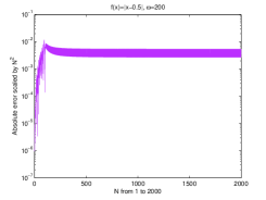
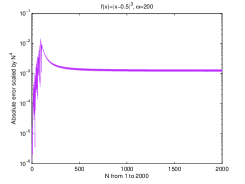
Figure 1: Absolute errors scaled by $N^{2}$ (left) and $N^{4}$ (right) for the integral (4.1) for the Clenshaw-Curtis-Filon method with $\omega=200$, $\alpha=0.2,\beta=0.4$, $N$ from $1$ to $2000$.

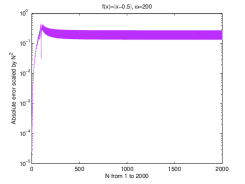
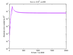
Figure 2: Absolute errors scaled by $N^{2}$ (left) and $N^{4}$ (right) for the integral (4.2) for the Clenshaw-Curtis-Filon method with $\omega=200$, $\alpha=0.2,\beta=0.4$, $N$ from $1$ to $2000$.

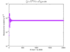
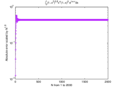
Figure 3: Absolute errors scaled by $N^{1.8}$ for the integral (4.3) (left) and integral (4.4) (right) for the Clenshaw-Curtis-Filon method with $\omega=200$, $\alpha=-0.8,\beta=-0.9$, $N$ from $1$ to $2000$.

From above two examples and Theorem 3.1, we can see that the Clenshaw-Curtis-Filon method is very efficient for the integral (1.1), and the accuracy can be improved by adding the number of the interpolation nodes. Also, the accuracy increases as $\omega$ increases.

5 Conclusion

In this paper, we present a Clenshaw-Curtis-Filon method for integral (1.1). The method is based on a special Lagrange interpolation polynomial at $N+1$ Clenshaw-Curtis points and can be computed by using $O(N\log N)$ operations. We first give a recurrence relation for the modified moments and present an efficient algorithm for the moments. Then, we show that the proposed method is uniformly convergent in $N$ for fixed $\omega$. The numerical examples illustrate the efficiency and accuracy for this method. Moreover, the error bound (3.9) is optimal on $N$ for fixed $\omega$. Here, the word “optimal” means that the asymptotic order can be attainable by some functions. Additionally, this result also holds for the Clenshaw-Curtis-Filon method for integral $\int_{a}^{b}f(x)(x-a)^{\alpha}(b-x)^{\beta}e^{i\omega x}dx$. It should be noted that the accuracy can be improved by adding the number of the interpolation nodes.

References

• [1] M. Abramowitz and I. A. Stegun, Handbook of Mathematical Functions, National Bureau of Standards, Washington, D.C., 1964.
• [2] G. Arkfen, Mathematical Methods for Physicists, third ed., Academic Press, Orlando, Fl, 1985.
• [3] G. Bao, W. Sun, A fast algorithm for the electromagnetic scattering form a large cavity, SIAM J. Sci. Comput. 27 (2005) 553–574.
• [4] H. Bateman, A. Erdélyi, Higher Transcendental Functions, Vol. I, McGraw-Hill, New York, 1953.
• [5] R. Chen, Numerical approximations to integrals with a highly oscillatory Bessel kernel, Appl. Numer. Math. 62 (2012) 636–648.
• [6] R. Chen, On the evaluation of Bessel transformations with the oscillators via asymptotic series of Whittaker functions, J. Comput. Appl. Math. 250 (2013) 107–121.
• [7] R. Chen, C. An, On evaluation of Bessel transforms with oscillatory and algebraic singular integrands, J. Comput. Appl. Math. 264 (2014) 71–81.
• [8] G. Dahlquist and A. Björck, Numerical Methods in Scientific Computing, SIAM, Philadelphia, 2007.
• [9] P. J. Davis and P. Rabinowitz, Methods of Numerical Integration, Second Edition, Academic Press, New York, 1984.
• [10] P. J. Davis and D.B. Duncan, Stability and convergence of collocation schemes for retarded potential integral equations, SIAM J. Sci. Comput. 42 (2004) 1167–1188.
• [11] A. Erdélyi, Asymptotic representations of Fourier integrals and the method of stationary phase, J. Soc. Ind. Appl. Math. 3 (1955) 17–27.
• [12] G. A. Evans and J. R. Webster, A high order progressive method for the evaluation of irregular oscillatory integrals, Appl. Numer. Math. 23 (1997) 205–218.
• [13] G. A. Evans and K. C. Chung, Some theoretical aspects of generalised quadrature methods, J. Complex. 19 (2003) 272–285.
• [14] L. Fox and I. B. Parker, Chebyshev Polynomials in Numerical Analysis, Oxford University Press, London, 1968.
• [15] I. S. Gradshteyn and I. M. Ryzhik, Table of Integrals, Series, and Products, 7th ed., Academic Press, New York, 2007.
• [16] http://functions.wolfram.com/HypergeometricFunctions/MeijerG/21/02/07/0001/.
• [17] D. Huybrechs and S. Vandewalle, A sparse discretisation for integral equation formulations of high frequency scattering problems, SIAM J. Sci. Comput. 29 (2007) 2305–2328.
• [18] H. Kang and S. Xiang, Efficient integration for a class of highly oscillatory integrals, Appl. Math. Comput. 218 (2011) 3553–3564.
• [19] D. Levin, Fast integration of rapidly oscillatory functions, J. Comput. Appl. Math. 67 (1996) 95–101.
• [20] D. Levin, Analysis of a collocation method for integrating rapidly oscillatory functions, J. Comput. Appl. Math. 78 (1997) 131–138.
• [21] J. C. Mason and D. C. Handscomb, Chebyshev Polynomials, Chapman and Hall/CRC, New York, 2003.
• [22] J. Oliver, The numerical solution of linear recurrence relations, Numer. Math. 11 (1968) 349–360.
• [23] S. Olver, Numerical approximation of vector-valued highly oscillatory integrals, BIT Numer. Math. 47 (2007) 637–655.
• [24] R. Piessens and M. Branders, Modified Clenshaw-Curtis method for the computation of Bessel function integrals, BIT Numer. Math. 23 (1983) 370–381.
• [25] T. J. Rivlin, Chebyshev Polynomials: From Approximation Theory to Algebra and Number Theory, 2nd ed., Wiley, New York, 1990.
• [26] L. N. Trefethen, Is Gauss quadrature better than Clenshaw-Curtis?, SIAM Rev. 50 (2008) 67–87.
• [27] L. N. Trefethen, Approximation Theory and Approximation Practice, SIAM, Philadelphia, 2013.
• [28] H. Wang, Convergence rate and acceleration of Clenshaw-Curtis quadrature for functions with endpoint singularities, arXiv:1401.0638, 2014.
• [29] S. Xiang and H. Wang, Fast integration of highly oscillatory integrals with exotic oscillators, Math. Comput. 79 (2010) 829–844.
• [30] S. Xiang, Y. Cho, H. Wang and H. Brunner, Clenshaw-Curtis-Filon-type methods for highly oscillatory Bessel transforms and applications, IMA J. Numer. Anal. 31 (2011) 1281–1314.
• [31] S. Xiang, G. He, Y. Cho, On error bounds of Filon-Clenshaw-Curtis quadrature for highly oscillatory integrals, Adv. Comput. Math. 41 (2015) 573–597.
• [32] S. Xiang, On the optimal rates of convergence for quadratures derived from Chebyshev points, arXiv:1308.4322, 2013.