Measurement of the binding energy of ultracold ⁸⁷Rb¹³³Cs molecules
using an offset-free optical frequency comb

Abstract

We report the binding energy of ⁸⁷Rb¹³³Cs molecules in their rovibrational ground state measured using an offset-free optical frequency comb based on difference frequency generation technology. We create molecules in the absolute ground state using stimulated Raman adiabatic passage (STIRAP) with a transfer efficiency of 88%. By measuring the absolute frequencies of our STIRAP lasers, we find the energy-level difference from an initial weakly-bound Feshbach state to the rovibrational ground state with a resolution of $\sim 5\text{\,}\mathrm{kHz}$ over an energy-level difference of more than $114\text{\,}\mathrm{THz}$; this lets us discern the hyperfine splitting of the ground state. Combined with theoretical models of the Feshbach state binding energies and ground-state hyperfine structure, we determine a zero-field binding energy of $h\times$114\,268\,135\,237(5)(50)\text{\,}\mathrm{kHz}$$. To our knowledge, this is the most accurate determination to date of the dissociation energy of a molecule.

Quantum gases of polar molecules have received great attention in recent years. Their long-range interactions and rich internal structure hold enormous potential in the fields of quantum many-body simulations Santos et al. (2000); Baranov et al. (2012), quantum computation DeMille (2002), ultracold chemistry Ospelkaus et al. (2010); Krems (2008) and precision measurement of fundamental constants Flambaum and Kozlov (2007); Isaev et al. (2010); Hudson et al. (2011); DeMille et al. (2008). It is only recently, however, that a limited selection of such molecules (KRb, RbCs, NaK, NaRb) have been successfully trapped at ultracold temperatures in their rovibrational ground state Ni et al. (2008); Takekoshi et al. (2014); Molony et al. (2014); Park et al. (2015); Guo et al. (2016), making them available for experimental study. These experiments all share a common technique for the production of molecules, in which atoms are first associated to form weakly bound molecules by tuning a magnetic field across a Feshbach resonance, and the molecules are then transferred optically to the ground state using stimulated Raman adiabatic passage (STIRAP) Gaubatz et al. (1990); Bergmann et al. (1998).

An accurate characterization of the internal structure of these molecules has been challenging both theoretically and experimentally. The most precise measurement so far of the binding energy of these molecules is for KRb Ni et al. (2008), where a frequency comb was used to measure the difference in laser frequency for the STIRAP transfer to a precision of $\pm$1\text{\,}\mathrm{MHz}$$ at a non-zero magnetic field. In ⁸⁷Rb¹³³Cs, the measurement precision has so far been approximately $20\text{\,}\mathrm{MHz}$, limited by the precision of wavemeters Debatin et al. (2011); Molony et al. (2014).

In this article, we present the most precise measurement of the binding energy $D_{0}$, or dissociation energy, of the lowest rovibrational state of the ⁸⁷Rb¹³³Cs $X^{1}\Sigma^{+}$ ground-state potential to date. We begin with a brief overview of the method we use to create samples of ultracold ground-state ⁸⁷Rb¹³³Cs molecules. We explain the working and stability of our novel frequency comb based on difference frequency generation (DFG), and how we use it to measure the $114\text{\,}\mathrm{THz}$ frequency difference between the STIRAP lasers. From this frequency difference we use theoretical models of the molecular structure to calculate the binding energy of the ⁸⁷Rb¹³³Cs molecule at zero magnetic field.

I Creating ground-state molecules

Details of our experimental setup may be found in our previous publications Harris et al. (2008); Jenkin et al. (2011); Cho et al. (2011); McCarron et al. (2011); Köppinger et al. (2014). Briefly, from a two-species magneto-optical trap we load both species into a magnetic trap Harris et al. (2008). We use forced RF evaporation Jenkin et al. (2011), followed by plain evaporation in a levitated optical trap ($\lambda=$1550\text{\,}\mathrm{nm}$$) Cho et al. (2011), to create a high phase-space density mixture of ${\sim}3.0\times 10^{5}$ atoms of each species at a temperature of $\sim 300\text{\,}\mathrm{nK}$ McCarron et al. (2011). Molecules are produced from this atomic mixture by sweeping the magnetic field across an interspecies Feshbach resonance at $197.10(3)\text{\,}\mathrm{G}$ at a rate of $250\text{\,}\mathrm{G}~{}\reciprocal{\mathrm{s}}$ Köppinger et al. (2014). After magnetoassociation, molecules populate the near-threshold $\ket{-1(1,3)s(1,3)}$ spin-stretched bound state of the potential $a^{3}\Sigma^{+}$ as shown in figure 1(b). Here, states are labeled as $\ket{n(f_{\rm{Rb}},f_{\rm{Cs}})L(m_{f_{\rm{Rb}}},m_{f_{\rm{Cs}}})}$, where $n$ is the vibrational quantum number counted downward from the dissociation threshold for the particular hyperfine $(f_{\rm{Rb}},f_{\rm{Cs}})$ manifold, and $L$ is the standard letter designation for the molecular rotational angular momentum quantum number Takekoshi et al. (2012). We transfer our molecules to the weakly bound $\ket{-2(1,3)d(0,3)}$ state by reducing the magnetic field to $\sim 180.5\text{\,}\mathrm{G}$, at which point the atoms and molecules are separated using the Stern-Gerlach effect (at a field gradient of $44\text{\,}\mathrm{G}~{}\reciprocal{\mathrm{c}\mathrm{m}}$), taking advantage of their different magnetic moments when the molecules are in this state. We then reduce the magnetic field gradient and ramp up the dipole trap to create a pure optical trap. Finally, the magnetic field is ramped to $\sim 181.5\text{\,}\mathrm{G}$ to transfer the molecules into a state which is suitable for transfer to the rovibrational ground state. This results in ${\sim}2500$ molecules in the $\ket{-6(2,4)d(2,4)}$ state at a temperature of $1.5\text{\,}\mathrm{\SIUnitSymbolMicro K}$.

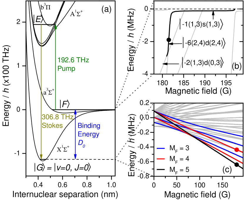
Figure 1: (Color online) ⁸⁷Rb¹³³Cs molecular states relevant to our experiment. (a) The position of the energy levels we use for STIRAP within the molecular potentials. The initial Feshbach state, intermediate excited state and ground state are labeled as $\ket{F}$, $\ket{E}$ and $\ket{G}$ respectively. (b) Molecular states close to dissociation. The dotted line is the Rb $\ket{f=1,m_{f}=1}$ + Cs $\ket{3,3}$ threshold. The black line shows the path followed by the molecules directly after magnetoassociation at the Feshbach resonance at $197.10(3)\text{\,}\mathrm{G}$. (c) Zeeman splitting of the ground state into 32 energy levels from total molecular nuclear spin $I^{\prime\prime}=2,3,4$ and $5$. Transitions to the highlighted states are allowed by selection rules. Dots indicate the states we address with our laser system.

The weakly bound molecules are transferred to the rovibrational ground state optically using STIRAP. We couple both the initial near-dissociation state and the ground state to a common excited state. This excited state is chosen to be the $\ket{\Omega^{\prime}=1,v^{\prime}=29,J^{\prime}=1}$ state, from the coupled $A^{1}\Sigma^{+}+b^{3}\Pi$ potential, because it has strong couplings to both the Feshbach and ground states Takekoshi et al. (2014). The pump and Stokes lasers are shown schematically in figure 1(a), and have frequencies of $192.6\text{\,}\mathrm{THz}$ ($1557\text{\,}\mathrm{nm}$) and $306.8\text{\,}\mathrm{THz}$ ($977\text{\,}\mathrm{nm}$) respectively. For coherent transfer, we narrow the linewidth of both pump and Stokes lasers to $<$1\text{\,}\mathrm{kHz}$$ by frequency stabilisation to a fixed-length high-finesse optical cavity constructed from ultra-low-expansion (ULE) glass by ATFilms. Continuous tuning is given by a pair of fibre-coupled electro-optic modulators. Further details of the laser system can be found in Gregory et al. (2015).

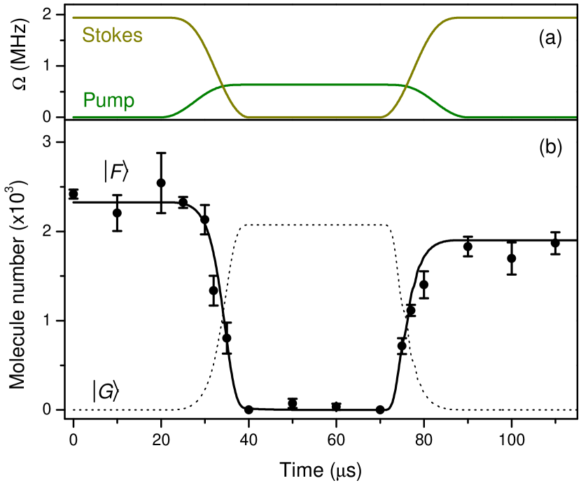
Figure 2: (Color online) STIRAP transfer to the molecular ground state and back. (a) Rabi frequency profile used for STIRAP transfer. (b) Experimentally measured population of the Feshbach state $\ket{F}$ throughout the transfer process. The sequence keeps the molecules in the ground state for $30\text{\,}\mathrm{\SIUnitSymbolMicro s}$ before transferring them back to the initial state for dissociation and absorption imaging. We show a numerical model of the Feshbach and ground state populations based on the Lindblad master equation for an open three-level system, including the effects of laser linewidth. The one-way transfer efficiency is 88%. The optical trap is switched off throughout the sequence.

We transfer the molecules to the ground state and back as shown in figure 2. This figure shows a model of the Lindblad master equation for an open three-level system, using our measured peak Rabi frequencies of $0.6\text{\,}\mathrm{MHz}$ and $1.9\text{\,}\mathrm{MHz}$ for the pump and Stokes transitions respectively. The details of this model will be presented in a separate publication. As the dipole trapping wavelength is close to the pump transition, it induces an AC Stark shift of $\sim 0.5\text{\,}\mathrm{MHz}$. This shift varies across the cloud because of the finite size of the molecular cloud and trapping beams, reducing the efficiency of the transfer. To avoid this we switch our dipole trap off for $200\text{\,}\mathrm{\SIUnitSymbolMicro s}$ during the STIRAP transfer to and from the ground state. This improves our one-way transfer efficiency from 50% Molony et al. (2014) to 88%, creating a sample of over 2000 molecules in the rovibrational ground state.

II Laser frequency measurement

We determine the binding energy with precision measurements of the pump and Stokes transition frequencies using a GPS-referenced frequency comb. Our frequency comb is the first of its kind, based on difference frequency generation technology developed by TOPTICA Photonics AG Telle (2005). In this comb, the amplified output of an Er:fiber oscillator is compressed using a silicon prism compressor and then spectrally broadened using a highly nonlinear photonic crystal fiber to make a supercontinuum spanning more than an optical octave. The comb teeth in the spectrum are given by $f=Nf_{\textrm{rep}}+f_{\textrm{CEO}}$. Two extreme parts of this supercontinuum are spatially and temporally overlapped in a nonlinear difference frequency generation (DFG) crystal. This cancels the carrier-envelope offset frequency ($f_{\textrm{CEO}}$) to produce an offset-free frequency comb spectrum at $1550\text{\,}\mathrm{nm}$ with a bandwidth of $\sim 100\text{\,}\mathrm{nm}$. Each comb tooth $N$ then has a frequency $f=Nf_{\textrm{rep}}$. This output is then extended to different wavelength ranges by nonlinear frequency shifting and frequency doubling. This method to cancel $f_{\textrm{CEO}}$ has the advantage of requiring no servo-loop feedback system, compared to the conventional $f-2f$ approach where the high-frequency noise components of $f_{\textrm{CEO}}$ cannot be canceled Fuji et al. (2004). The characterization of the phase noise of different comb teeth confirms the elastic tape model Benkler et al. (2005) with a fixed point at zero frequency Puppe et al. (2016).

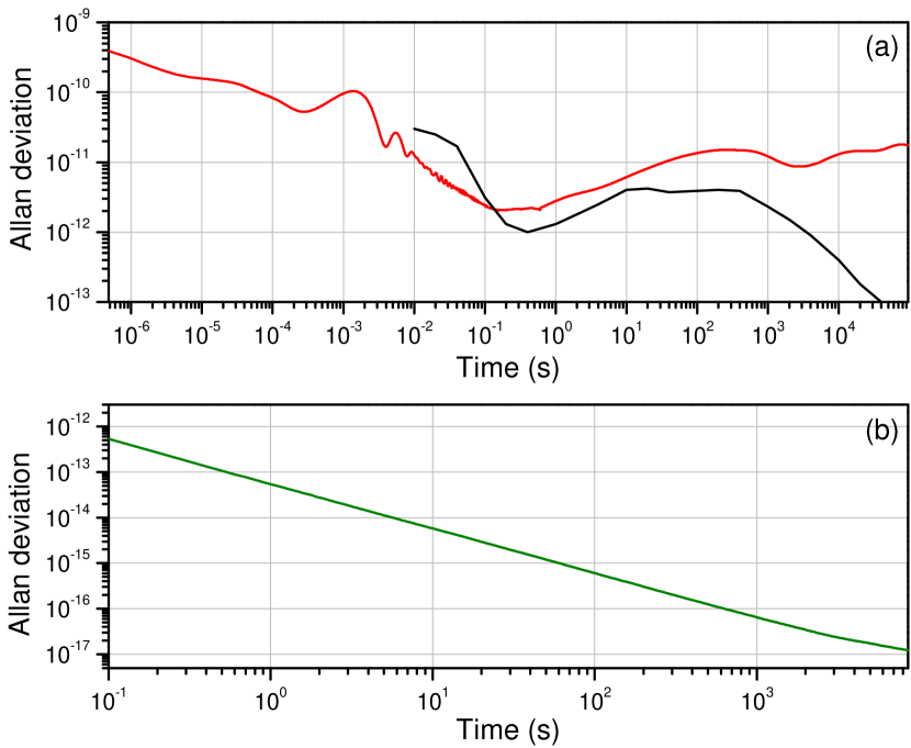
Figure 3: (Color online) Measurements of the stability of the frequency comb. (a) Allan deviation (AD) of a beat between the frequency comb and a laser stabilized to the Rb 5S${}_{1/2}(f$=2)$\rightarrow$5P${}_{3/2}(f^{\prime}$=3) transition (red), and the AD of the GPS-referenced $10\text{\,}\mathrm{MHz}$ oscillator (black) to which the comb is locked. (b) AD of the beat signal between two identical DFG combs locked to a common reference. The beat was recorded at a wavelength of $1556\text{\,}\mathrm{nm}$ via a transfer oscillator Puppe et al. (2016).

The frequency comb is seeded by a mode-locked Er:fibre laser with an $80\text{\,}\mathrm{MHz}$ repetition rate, whose 10th harmonic is locked to an $800\text{\,}\mathrm{MHz}$ ultra-low-noise oven-controlled RF oscillator, which in turn is locked to a $10\text{\,}\mathrm{MHz}$ GPS reference (Jackson Labs Fury). We have measured the absolute stability of the comb locked to the GPS reference by recording a beat note between a comb tooth and a laser stabilized to the Rb 5S${}_{1/2}(f$=2)$\rightarrow$5P${}_{3/2}(f^{\prime}$=3) line. Figure 3(a) shows the Allan deviation (AD) of the beat signal, compared to the AD of the GPS referenced oscillator to which the comb is locked. The AD of the beat follows a similar trend to the reference signal but deviates at longer time scales. This deviation is due to the drift in the lock-signal offset of the laser locked to the Rb spectroscopy line and is commonly observed over such time scales. These results show that measuring uncertainties down to $10^{-11}$ is practical with our comb system.

To quantify the lock noise of the comb, we measure the AD of a beat signal between two combs locked to a common RF reference. We observe an overall AD lower than the reference signal with no similarity to the AD of the reference signal (figure 3(b)). This indicates that the AD of the reference RF is completely canceled in this measurement and the AD related to lock noise is much smaller than that. Therefore we can consider the AD of the GPS signal at time scales greater than our experimental cycle to calculate the resulting deviation on the repetition rate.

The frequency difference between the two STIRAP lasers is measured with comb teeth separated by $\delta N=$(306.8-192.6)\text{\,}\mathrm{THz}$/$80\text{\,}\mathrm{MHz}$\sim 10^{6}$, so the uncertainty in the GPS clock frequency must be less than $10\text{\,}\mathrm{mHz}$ if we are to maintain an uncertainty in our measured laser frequency of less than $10\text{\,}\mathrm{kHz}$. The AD over time scales shorter than the experimental cycle will add to the statistical error of the molecular round-trip signal. However, the AD over longer time scales will lead to a systematic offset in our measurements. From the specifications of the GPS reference we calculate that, over the course of one measurement, the AD leads to a systematic uncertainty of $\pm 23\text{\,}\mathrm{Hz}$ on the frequency difference between the two lasers. This is negligible compared to the other sources of uncertainty described later.

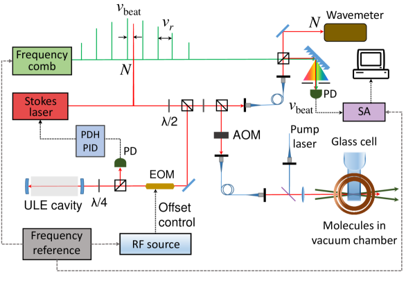
Figure 4: (Color online) Schematic diagram of the experiment to carry out spectroscopy while recording the beat note ($\nu_{\text{beat}}$) of the STIRAP lasers with the optical frequency comb. The beat signal between each STIRAP laser and the nearest comb line ($N$) is detected on a photodiode which is connected to a spectrum analyzer (SA). Both STIRAP lasers are frequency stabilized to a common ULE cavity using the Pound-Drever-Hall method Black (2001). Continuous tuning of each laser is provided by varying the RF driving frequency of a broadband fibre-coupled electro-optic modulator (EOM). The light reaching the molecules is offset by $80\text{\,}\mathrm{MHz}$ from that sent to the frequency comb by an acousto-optic modulator (AOM) which modulates the intensity of the light. Further details of the frequency stabilization and tuning of the STIRAP lasers can be found in Gregory et al. (2015). The frequency comb, spectrum analyzers and EOM driver are all referenced to the same $10\text{\,}\mathrm{MHz}$ GPS disciplined oscillator. The figure shows the setup for the Stokes laser; the setup for the pump laser is identical.

The absolute frequency of the lasers is measured by beating light from each of the STIRAP lasers with the nearest tooth of the optical frequency comb. A schematic diagram of the optical setup used to measure the beat note and the comb tooth number is shown in figure 4. The beat note is recorded on a spectrum analyzer (Agilent N9320B for the Stokes, Agilent N1996 for the pump), which is referenced to the same $10\text{\,}\mathrm{MHz}$ GPS clock as the comb. The frequency of the beat note is averaged and recorded over each three-second interval. We identify the nearest comb tooth ($N$) using a wavemeter with an absolute accuracy of $30\text{\,}\mathrm{MHz}$ (High Finesse WS-U), which we calibrate with lasers locked to well-known spectral lines in Rb, Cs and Sr.

The light reaching the molecules is offset from that sent to the frequency comb by a pair of acousto-optic modulators (AOMs), at $+80\text{\,}\mathrm{MHz}$ and $-80\text{\,}\mathrm{MHz}$ for the pump and Stokes respectively. These provide the analog intensity ramps for STIRAP, and are driven by ISOMET 532B fixed-frequency driver/amplifiers. We measure the accuracy of the absolute frequency of these drivers on a spectrum analyser (Agilent N1996 referenced to the $10\text{\,}\mathrm{MHz}$ GPS clock) and find a constant offset of $-705.0(3)\text{\,}\mathrm{Hz}$ from the nominal $80\text{\,}\mathrm{MHz}$. The statistical uncertainty on this offset is negligible.

III Energy difference measurement

Maximum STIRAP transfer efficiency is achieved when the laser frequencies meet the two-photon resonance condition, while any common detuning of both lasers has relatively little effect on the efficiency Bergmann et al. (1998); Gregory et al. (2015). By scanning their frequency difference and observing where we get maximum transfer efficiency, we determine the energy difference between the initial state $\ket{F}$ and final state $\ket{G}$.

To measure the energy difference, we fix the frequency of the pump laser on resonance with the Feshbach and intermediate states. We then vary the frequency of the Stokes laser and measure the efficiency of the STIRAP transfer. The beat notes of both lasers with the optical frequency comb are measured throughout. For each data point we subtract the pump and Stokes absolute frequencies measured with the comb, and add the shifts from the AOMs, to get an absolute frequency difference. This gives us a peak as a function of Stokes frequency which we fit to determine the energy difference between the initial and final states, as shown in figure 5. The optimal Stokes frequency is determined over $\sim 4$ hours.

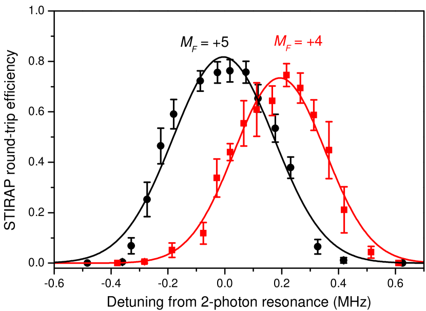
Figure 5: (Color online) STIRAP transfer to different hyperfine sub-levels. The STIRAP round-trip transfer efficiency changes with the frequency difference of the pump and Stokes lasers for horizontal (black circles) and vertical (red squares) Stokes polarizations at a magnetic field of $\sim 181.5\text{\,}\mathrm{G}$. Black circles show the transfer to the ${M_{F}=+5}$ state, while red squares show the ${M_{F}=+4}$ state. Gaussian fits give a separation between the states of $0.194(10)\text{\,}\mathrm{MHz}$.

The precision with which we can locate the two-photon resonance is limited by the shot-to-shot noise in the number of molecules which we produce. This noise results in the vertical error bars seen in figure 5. The uncertainties in the detuning (the horizontal error bars) are too small to be seen. A Gaussian fit gives an uncertainty on the center of the spectroscopic feature of around $\pm 8\text{\,}\mathrm{kHz}$. The magnetic field is measured before and after each complete measurement using the microwave transition frequency between the $\ket{f=3,m_{f}=+3}$ and $\ket{4,+4}$ states in atomic Cs.

We found the same frequency difference between the pump and Stokes transition, within our experimental uncertainty, when using $\ket{\Omega^{\prime}=0,v^{\prime}=35,J^{\prime}=1}$ as an alternative intermediate state. This measurement was carried out using two-photon spectroscopy (where both the pump and Stokes light are pulsed on simultaneously) as the coupling strengths are not high enough for efficient STIRAP transfer. The experimental procedure for the two-photon spectroscopy of the ground state has been discussed previously by Molony et al. (2014) and Gregory et al. (2015). This method, and the different transition strengths and linewidths, results in a much wider spectroscopic signal, leading to much larger uncertainties on the two-photon resonance.

IV Binding Energy Calculation

We will now combine the measured energy difference and magnetic field with theoretical models, to determine the energy difference between the degeneracy-weighted centres of the atomic and molecular hyperfine manifolds. We must correct for several shifts which are included in our measurement: the atomic hyperfine splittings, the Zeeman shifts of the $\ket{1,1}$ and $\ket{3,3}$ atomic states, the binding energy of the Feshbach molecule relative to these atomic states, and the molecular ground-state hyperfine splitting and Zeeman shift. The effects of all of these shifts are summarised in table 1. We will discuss each of these below.

Source	Correction (MHz) 000	Error (MHz)
$\nu_{\text{Stokes}}-\nu_{\text{pump}}$	114 258 363.067 000	0.006
Feshbach binding energy	1.838 000
Rb Zeeman	194.084 000
Cs Zeeman	134.353 000
RbCs Zeeman	$-$0.734 000
Total Zeeman		0.013
Cs hyperfine	$\frac{9}{16}\times 9\,192.631\,770$	$\equiv 0$
Rb hyperfine	$\frac{5}{8}\times 6\,834.682\,611$	$<10^{-10}$
RbCs hyperfine ($I$=5)	0.091 000
Binding energy	114 268 135.230 000	0.014

Table 1: All the corrections, and their respective experimental errors, which must be added to our measurement of the energy difference $\nu_{\text{Stokes}}-\nu_{\text{pump}}$ to give the energy difference between the degeneracy-weighted hyperfine centroids of the free atoms and the RbCs rovibrational ground state, i.e. the binding energy. The uncertainty in the Zeeman shift is from the uncertainty in the measured magnetic field. Additional systematic uncertainties apply as explained in the text. The values shown are from the second measurement in figure 7 at a magnetic field $181.538(6)\text{\,}\mathrm{G}$ driving a transition to the $M_{F}=5$ hyperfine ground state. All values are in MHz.

The Cs ground-state hyperfine splitting at zero field comes directly from the definition of the second, while the Rb splitting has been measured to $<$100\text{\,}\mathrm{\SIUnitSymbolMicro Hz}$$ Bize et al. (1999). These are weighted by the degeneracies of the atomic hyperfine states to give the distance to the $5^{2}S_{1/2}+6^{2}S_{1/2}$ center. The atomic Zeeman splittings are calculated from the standard atomic Hamiltonian. The electron spin, electron orbital and nuclear g-factors are the CODATA recommended values Mohr et al. (2014). We assume the theoretical errors on these models are negligible.

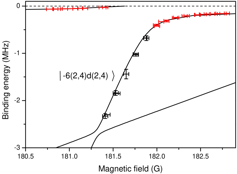
Figure 6: (Color online) The calculated positions of the highest-lying bound states for ⁸⁷Rb¹³³Cs (solid black lines) together with the positions measured by free-bound magnetic-field modulation spectroscopy. The measurements included in the analysis of the required shifts of the binding energy (see main text) are colored black, and the other data points in the set are colored red. There are 9 points included in the fit; some of them nearly overlap. Data taken from Takekoshi et al. (2012).

We estimate the binding energy of the Feshbach state with respect to the $\ket{1,1}+\ket{3,3}$ threshold by combining the measurements and the coupled-channel model of reference Takekoshi et al. (2012), as shown in figure 6. There are 9 experimental points for the $|-6(2,4)d(2,4)\rangle$ state between 181.4 G and 181.9 G , and the coupled-channel model systematically underestimates the binding energies by $0.09(4)\text{\,}\mathrm{MHz}$. For the present work, we recalculate the binding energies from the coupled-channel model as a function of $B$ and increase the resulting binding energies by this amount. We include the $40\text{\,}\mathrm{kHz}$ uncertainty as a theoretical contribution to the final value for the ground-state binding energy.

The $J=0$ rovibrational ground state has 4 hyperfine levels with nuclear spins $I=2,3,4,5$. In the presence of a magnetic field, these are split into 32 hyperfine and Zeeman states originating from the nuclear spin coupling to the magnetic field. These energy levels were calculated using the molecular Hamiltonian and parameters in reference Aldegunde et al. (2008) and are plotted in figure 1(c). We subtract both the hyperfine and the Zeeman shifts to give the binding energy of the ground-state hyperfine centroid, i.e. the zero of the energy axis in figure 1(c).

There are also theoretical uncertainties associated with the model of the ground-state hyperfine structure. The hyperfine splitting of the $I=2,3,4,5$ states is determined almost entirely by the scalar nuclear spin-spin coupling constant $c_{4}$, which was calculated using density-functional theory (DFT) by Aldegunde et al. (2008). We estimate that the uncertainty on $c_{4}$ is $\pm 30\%$, giving an uncertainty of $\pm 27\text{\,}\mathrm{kHz}$ on the position of the $I=5$ state relative to the degeneracy-weighted hyperfine centroid. The Zeeman shift is determined by the nuclear shielding constants, also from DFT Aldegunde et al. (2008), but we estimate that the uncertainties in these shieldings cause an uncertainty of only $\pm 1\text{\,}\mathrm{kHz}$. We combine these ground-state uncertainties with the theoretical uncertainty on the model of the Feshbach binding energy to give a total theoretical error of $50\text{\,}\mathrm{kHz}$. This is included as a separate “theoretical” uncertainty in the final value of the ground-state binding energy.

We selectively address different hyperfine sublevels of the rovibrational ground state by changing the polarization of the Stokes laser Takekoshi et al. (2014) while keeping the pump laser polarization fixed parallel to the quantization axis. The weakly bound state from which we begin our STIRAP transfer has a total angular momentum projection quantum number $M_{F}=+4$. In the case of Stokes polarization parallel to the quantization axis, we drive $\pi$ transitions and address a ground state where the $M_{F}$ value is unchanged. If, on the other hand, the Stokes polarization is perpendicular to the quantization axis, we drive $\sigma^{\pm}$ transitions and address ground states with either $M_{F}=+3$ or $M_{F}=+5$.

In figure 5, we see the effect of scanning the Stokes laser frequency on the efficiency of STIRAP transfer for both parallel and perpendicular polarizations. The coupling strengths to the hyperfine ground states are such that we have sufficient laser power to populate only two of the available hyperfine states, which are separated in energy by $0.194(10)\text{\,}\mathrm{MHz}$. The measured energy difference, in combination with knowledge of the states accessible with different Stokes polarizations, allows us to identify the two states as indicated in figure 1(c), agreeing with previous results Takekoshi et al. (2014). Both of these Zeeman states correlate with the $I=5$ hyperfine state. Because of mixing between the $I=4$ and $I=5$ states in a magnetic field, the measured splitting of $0.194(10)\text{\,}\mathrm{MHz}$ has some dependence on the spin-spin coupling constant $c_{4}$. It corresponds to a value $c_{4}=$0.023(7)\text{\,}\mathrm{kHz}$$, which agrees within its error bars with the value of $0.01734\text{\,}\mathrm{kHz}$ from DFT calculations Aldegunde et al. (2008) and is also consistent with our attribution of an uncertainty of 30% to the latter value. We note that at a field of $\sim 181.5\text{\,}\mathrm{G}$ the $M_{F}=+5$ state is the lowest-energy sublevel, as shown in figure 1(c).

We must also consider the effect of the uncertainty in the magnetic field. We have considered the atomic and molecular Zeeman shifts separately above, but with the uncertainty in the field they must be considered together. We multiply the uncertainty in the measured field by the difference in magnetic moment between the Feshbach and ground states to give the associated uncertainty in the binding energy. This is shown in table 1, and is added to the uncertainty from the frequency difference measurement above to give the total statistical uncertainty on the binding energy.

V Measurement campaign

We have repeated the measurement outlined in the section IV five times on different days, and observed similar results for the energy difference each time, within experimental errors. In this section, we combine these measurements to give a value for the binding energy $D_{0}$. All five measurements are summarised in figure 7, and the precise values for each measurement are shown in table 2.

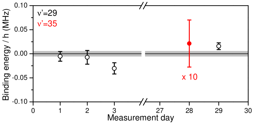
Figure 7: (Color online) Binding energy of the ⁸⁷Rb¹³³Cs molecule measured on different days, with experimental error bars. The vertical scale is offset by the mean value of $114\,268\,135.237\text{\,}\mathrm{MHz}$. The gray shaded region represents the $5\text{\,}\mathrm{kHz}$ experimental error on the mean. Black (red) data points show the binding energy calculated from two-photon spectroscopy via $\ket{\Omega^{\prime}=1,v^{\prime}=29,J^{\prime}=1}$ ($\ket{\Omega^{\prime}=0,v^{\prime}=35,J^{\prime}=1}$) as the intermediate state. The $\ket{\Omega^{\prime}=0,v^{\prime}=35,J^{\prime}=1}$ measurement and error bar have been divided by 10 for clarity. The larger experimental errors in two-photon spectroscopy via the $\ket{\Omega^{\prime}=0,v^{\prime}=35,J^{\prime}=1}$ state are due to the poor signal-to-noise ratio of the molecular spectroscopy signal.

The measurement shown in red in figure 7 uses the $\ket{\Omega^{\prime}=0,v^{\prime}=35,J^{\prime}=1}$ intermediate state. The polarisations are such that we expect to address the $M_{F}=3,5$ states, but the large spectroscopic linewidth means this measurement does not resolve the ground-state hyperfine structure. The main purpose of this measurement is to confirm that we have identified the frequency comb tooth correctly. The other four measurements use the $\ket{\Omega^{\prime}=1,v^{\prime}=29,J^{\prime}=1}$ state in the coupled $A^{1}\Sigma^{+}+b^{3}\Pi$ potential. Of these, three are measured with the $M_{F}=5$ ground-state hyperfine level, and one uses the $M_{F}=4$ state.

Following the procedure in the previous sections, we calculate values for binding energies for each measurement. Taking a weighted mean we get a final value for the binding energy of ⁸⁷Rb¹³³Cs of

$$D_{0} =h\times$114\,268\,135\,237(5)(50)\text{\,}\mathrm{kHz}$$$

$$=hc\times$3811.574\,714\,03(16)(200)\text{\,}\reciprocal{\mathrm{c}\mathrm{m}}$.$$

The first uncertainty arises from the statistical experimental error and the second one arises from the theoretical uncertainties in the coupled-channel model and the ground-state hyperfine splitting. The uncertainty in the final value of the binding energy is dominated by the theoretical uncertainties. Our experimental frequency measurements are more accurate by one order of magnitude.

Polarization	$M_{F}$	$\nu_{\text{Stokes}}-\nu_{\text{pump}}$ (MHz)	$B$ (G)	$D_{0}/h$ (MHz)
$V_{\text{P}},V_{\text{S}}$	4	114 258 362.874(8)	181.542(3)	114 268 135.232(10)
$V_{\text{P}},H_{\text{S}}$	5	114 258 363.067(6)	181.538(6)	114 268 135.230(14)
$V_{\text{P}},H_{\text{S}}$	5	114 258 363.075(8)	181.552(4)	114 268 135.207(12)
$V_{\text{P}},H_{\text{S}}$*	5	114 258 363.2(5)	181.510(3)	114 268 135.4(5)
$V_{\text{P}},H_{\text{S}}$	5	114 258 363.048(5)	181.519(2)	114 268 135.253(7)

Table 2: Summary of each independent measurement of the binding energy in the ground state. Both the magnetic field and the polarization of the pump light are vertical ($V_{\text{P}}$). The Stokes light may be either vertical ($V_{\text{S}}$) or horizontal ($H_{\text{S}}$) to access ground-state hyperfine levels with either $M_{F}=4$ or $M_{F}=5$. For each measurement we show the absolute frequency difference measured for each laser ($\nu_{\text{Stokes}}-\nu_{\text{pump}}$), the magnetic field during that measurement ($B$), and the binding energy of the ground state at zero field ($D_{0}$). An additional $0.05\text{\,}\mathrm{MHz}$ theoretical uncertainty applies to the binding energies, as explained in the text. An asterisk* indicates a measurement using two-photon spectroscopy via the intermediate $\ket{\Omega^{\prime}=0,v^{\prime}=35,J^{\prime}=1}$ state. All other measurements rely on optimization of the round-trip STIRAP efficiency via the intermediate $\ket{\Omega^{\prime}=1,v^{\prime}=29,J^{\prime}=1}$ state.

This value is a 500-fold improvement in accuracy over previous measurements averaging $3811.5759(8)\text{\,}\reciprocal{\mathrm{c}\mathrm{m}}$ Debatin et al. (2011); Molony et al. (2014). The most precise determinations of a molecular binding energy we know of are precisions of $\Delta E/E\sim 10^{-8}$. These are in ⁴⁰K⁸⁷Rb, which is measured with $8\times 10^{-9}$ precision at a finite magnetic field Ni et al. (2008), and $\textrm{H}_{2}$ with $1\times 10^{-8}$ precision Liu et al. (2009). Our fractional uncertainty is $4\times 10^{-10}$, and improved models and measurements of the Feshbach and ground-state structure could reduce this as far as $5\times 10^{-11}$.

VI Conclusions

We have measured the binding energy of the ⁸⁷Rb¹³³Cs molecule as $h\times$114\,268\,135\,237(5)(50)\text{\,}\mathrm{kHz}$$ using an optical frequency comb based on difference-frequency generation Telle (2005); Fehrenbacher et al. (2015). The results for different intermediate states $\sim 1.65\text{\,}\mathrm{THz}$ apart agree within their experimental uncertainty and we are able to resolve the nuclear Zeeman splitting of the molecular ground state. The accuracy of our ground-state binding energy measurement is limited by uncertainties in the theoretical models of the molecular structure. This is, to our knowledge, the most accurate determination to date of the dissociation energy of a molecule. The ability to measure molecular transitions with high precision is also potentially relevant to searches for variations in fundamental constants such as the electron-proton mass ratio DeMille et al. (2008).