On the spontaneous time-reversal symmetry breaking in synchronously-pumped passive Kerr resonators

Abstract

We study the spontaneous temporal symmetry breaking instability in a coherently-driven passive optical Kerr resonator observed experimentally by Xu and Coen in Opt. Lett. 39, 3492 (2014). We perform a detailed stability analysis of the Lugiato-Lefever model for the optical Kerr resonators and analyze the temporal bifurcation structure of stationary symmetric and the emerging asymmetric states as a function of the pump power. For intermediate pump powers a pitchfork loop is responsible for the destabilization of symmetric states towards stationary asymmetric ones while at large pump powers we find the emergence of periodic asymmetric solutions via a Hopf bifurcation. From a theoretical perspective, we use local bifurcation theory in order to analyze the most unstable eigenmode of the system. We also explore a non-conservative variational approximation capturing, among others, the evolution of the solution’s amplitude, width and center of mass. Both methods provide insight towards the pitchfork bifurcations associated with the symmetry breaking.

I Introduction

Spontaneous symmetry breaking (SSB) is the basis for many phase transitions and account for effects including ferromagnetism, superconductivity, and convection cells zurek ; stanley . SSB has been widely observed in nonlinear optics and is at the heart of numerous fundamental phenomena including, but not limited to, asymmetric dynamics in coupled mode models kenkre , optical waveguide arrays Boris_Gisin_Kaplan_PRE_2000 , coupled nonlinear micro-cavities Haelterman_OE_2006 , and photonic lattices Panos_PLA_2005 . For a detailed exposition of numerous recent directions within the subject from the perspective of nonlinear phenomena, see Ref. Boris_SSB_book . SSB is not restricted to Hamiltonian (conservative) systems. For instance, over the past few years, it has also played a prominent role in the context of parity-time, so-called PT, symmetric systems kivshar ; yang bearing a balanced interplay between gain and loss. There, it is responsible for the emergence of “ghost” states both in the case of dimers (and more generally oligomers) cartarius , but also in that of continuous media rcg:85 ; rcg:88 , where they can be responsible for the destabilization and bifurcations associated with solitary waves and vortices.

A remarkable example of SSB in a dissipative system was observed by Xu and Coen in Ref. XuCoen where a system composed of a synchronously-pumped passive optical resonator filled with a Kerr nonlinear material was experimentally explored. This system exhibits a temporal SSB instability in which the discrete time-reversal symmetry is broken and symmetric states become unstable in favor of stable asymmetric states. It is the purpose of the present manuscript to complement the experimental and numerical analysis of Ref. XuCoen by putting forward a thorough analytical (and partially numerically assisted) understanding of the origin and manifestation of SSB (and additional possible, such as Hopf) bifurcations in this system.

We consider, as in Ref. XuCoen , a model for a passive Kerr resonator in an optical fiber ring cavity described by a single partial differential equation (PDE), resulting from an averaging procedure, of the nonlinear Schrödinger (NLS) equation-type, known as the mean-field Lugiato-Lefever (LL) model LL ; LLE . The LL equation, taking into account gain and loss in the system, can be cast, in non-dimensional form, as XuCoen ; XuCoenRef22a ; XuCoenRef22b :

$$\frac{\partial E(z,\tau)}{\partial z}=\left[-1+i(\left|E\right|^{2}-\Delta)-i\eta\frac{\partial^{2}}{\partial\tau^{2}}\right]E+S(\tau),$$ (1)

where $z$ is the slow evolution variable of the intracavity field $E$ over successive normalized cavity round-trips and $\tau$ describes the temporal variable in the dependence of the intracavity pulse envelope. The terms in the right-hand-side of Eq. (1) correspond, respectively, to cavity losses $(-E)$, Kerr nonlinearity $(i\left|E\right|^{2}E)$, cavity phase detuning $(-i\Delta E)$, chromatic dispersion $(-i\eta\frac{\partial^{2}}{\partial\tau^{2}}E)$, and external pumping $(S(\tau))$. Within this non-dimensional form XuCoenRef22a ; XuCoenRef22b , the cavity phase detuning corresponds to $\Delta=\delta_{0}\alpha$, where $\alpha$ is half the fraction of power lost per round-trip and the cavity finesse is $\mathscr{F}=\pi/\alpha$, and $\delta_{0}=2m\pi-\phi_{0}$ where $\phi_{0}$ is the overall cavity round-trip phase shift and $m$ is the order of the closest cavity resonance. The sign of the group-velocity dispersion coefficient of the fiber is $\eta$ which is taken as $\eta=-1$ for our analysis with self-focusing nonlinearity. The field envelope of the external pump pulses, $S(\tau)$, is modeled by a symmetric chirp-free Gaussian pulse given by $S(\tau)=\sqrt{X}\exp\left[-(\tau/T_{0})^{2}\right]$, with $T_{0}=2.3$ as in the experiments of Ref. XuCoen .

For the SSB instability of the passive Kerr cavity, the pump pulse field profile is temporally symmetric, $S(\tau)=S(-\tau)$, and the model is symmetric under a time reversal transformation, $\tau\rightarrow-\tau$, yet it admits asymmetric solutions, as described in Ref. XuCoen . The associated pitchfork bifurcation illustrates that at low pump peak power $X$, the solutions are symmetric in time; however, above a certain pump peak power threshold the symmetric states become unstable while stable asymmetric states emerge. The particular experimental parameters of Ref. XuCoen generate, as $X$ is increased further, a reverse pitchfork as well, in which the asymmetric states collide and disappear while the symmetric state recovers its stability. We examine this SSB-induced instability interval in the passive Kerr resonator modeled by Eq. (1) by means of a non-conservative variational approximation (NCVA) JuliaNCVA and further through a center manifold reduction MH-Iooss enabling the analysis of the dominant associated eigenmodes (responsible for determining the spectral stability of the system). It is relevant to mention at this point that a thorough bifurcation analysis for a LL equation in the case of constant external pumping was recently carried out in Ref. LLE_french_PRA , showing quite complex bifurcation scenarios in both the anomalous and normal dispersion regimes.

In the NCVA context, our aim is to apply a variational method based on well-informed ansätze in the corresponding Lagrangian of the system. The ansätze reduce the complexity of the original infinite-dimensional problem to a few degrees of freedom capturing the principal, static and dynamic characteristics of the system. This method attempts to project the infinite-dimensional dynamics of Eq. (1) into a low-dimensional dynamical system that qualitatively and, to some extent, quantitatively captures SSB bifurcations and the solutions emanating from it. However, it is important to note that traditional variational methods rely on the existence of a Lagrangian or Hamiltonian structure for closed systems for which equations of motion can be derived. Nonetheless, recently, Galley ref1 offered an approach allowing to extend the method to open, non-conservative systems which in turn was generalized to dissipative (containing gain and loss) NLS-type systems in Ref. JuliaNCVA inspired by the work of Ref. ref4 on the extension of Galley’s formalism to PT-symmetric variants of field theories. It is this variant of the NCVA that we will explore in the present setting.

Our analysis of the observed SSB will be complemented by center manifold reductions. The latter are extensively used in the analysis of local bifurcations. Starting from a dynamical systems formulation of the bifurcation problem, the reduction to a center manifold provides the lowest dimensional dynamical system which fully describes the original dynamics close to a bifurcation point. We use this method to analyze the two pitchfork bifurcations which arise in Eq. (1) as $X$ is increased. As a result we obtain, in both cases, a reduced scalar ordinary differential equation which captures the bifurcating dynamics. The first two coefficients in the expansion of the reduced scalar field, which are computed numerically here, determine the type of the bifurcation. They are also essential in the computation of the bifurcating asymmetric states and of the local temporal dynamics.

The paper is organized as follows. In Sec. II we identify the equilibria and study their stability by means of a spectral analysis of the linearization problem; this is a perspective that was absent in the original work of Ref. XuCoen and which, we argue, provides a more systematic insight into the stability (and the potential instabilities) of the system. In doing so, we recover the forward and reverse pitchfork bifurcations (i.e., a pitchfork loop) observed in Ref. XuCoen as well as identify a Hopf bifurcation for larger pump power giving rise to asymmetric, stable, periodic solutions; the latter is an important feature of dynamical interest in its own right and should be, in principle, observable in suitable extensions of the experiments of XuCoen . Section III is devoted to the NCVA approach. In Sec. III.1 we provide a brief description of the NCVA approach and its formulation within the LL model. Section III.2 is devoted to the application of the NCVA to capture the SSB bifurcation for physically relevant parameters values of the system as in Ref. XuCoen . In Sec. IV we complement our understanding of the pitchfork loop bifurcation by giving the local bifurcation analysis which is effective towards qualitatively and quantitatively describing the emerging asymmetric solutions close to the pitchfork bifurcation points. Finally, in Sec. V we summarize our findings and we provide possible avenues for future research.

II The Full Model: Equilibria, Stability and Bifurcations

In this section, we follow the various equilibria of Eq. (2) as the peak pump power, $X$, is varied and determine their stability. Let us recast Eq. (1) into the simpler form

$$iu_{z}+u_{\tau\tau}+(|u|^{2}-\Delta)u=-iu+iS(\tau),$$ (2)

which corresponds to the NLS with additional non-conservative terms (namely the terms in the right-hand side). In what follows, we identify stationary solutions, $u(z,\tau)=u_{0}(\tau)$ of Eq. (2) by numerically solving the steady-state equation

$$u_{0,\tau\tau}+(|u_{0}|^{2}-\Delta)u_{0}=-iu_{0}+iS(\tau).$$ (3)

It is relevant to mention that since the forcing (pump) term in Eq. (1) is independent of the field’s wavefunction, it is necessary for the steady state to be independent of $z$ (i.e., here the detuning parameter $\Delta$ plays the role of the frequency). It is also worth mentioning that the steady state is, in general, complex which, as we will see below, is crucial for the steady state to sustain itself through a stationary flow from the gain to the loss portions of the solution.

Let us now consider the stability of a steady state $u_{0}$ by means of a spectral stability analysis. Specifically, small perturbations of order $\mathcal{O}(\epsilon)$, with $0<\epsilon\ll 1$, to the stationary solutions are introduced in the form:

$$u(z,\tau)=u_{0}(\tau)+\epsilon[a(\tau)e^{\lambda z}+b^{*}(\tau)e^{\lambda^{*}z}],$$

and substituted into Eq. (2). Then, the ensuing linearized equations are solved to $\mathcal{O}(\epsilon)$, leading to the eigenvalue problem:

$$i\lambda\begin{pmatrix}a(z)\\ b(z)\end{pmatrix}=\begin{pmatrix}M_{1}&M_{2}\\ -M_{2}^{*}&-M_{1}^{*}\end{pmatrix}\begin{pmatrix}a(z)\\ b(z)\end{pmatrix},$$ (4)

for the eigenvalues $\lambda$ and associated eigenvector $\xi=(a(z),b(z))^{\mathrm{T}}$, where $(\cdot)^{*}$ denotes complex conjugation and $M_{1}$ and $M_{2}$ are the following operators:

$$M_{1} =-\partial_{\tau}^{2}-2|u_{0}|^{2}+(\Delta-i),$$

$$M_{2} =-u_{0}^{2}.$$ (5)

The stationary solutions are linearly unstable provided Re$(\lambda)>0$. When unstable, the dynamics of the respective instabilities can be monitored through direct numerical simulations of Eq. (2).

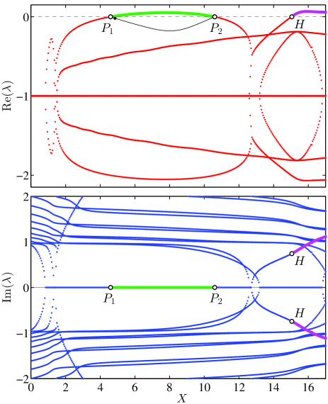
Figure 1: Linearization spectrum for the symmetric and asymmetric steady state solutions of the Lugiato-Lefever equation (2) as the pump power $X$ is varied for $\Delta=0.92$ and $T_{0}=2.3$. The top and bottom panels depict, respectively, the real and imaginary parts of the eigenvalues. Stable symmetric solutions bearing Re$(\lambda)<0$ are depicted by small (red) dots in the top panel while unstable symmetric solutions are depicted with thick solid lines. The thick (green) solid line between the points $P_{1}$ and $P_{2}$ represents the unstable solutions through forward ($P_{1}$) and reverse ($P_{2}$) pitchfork bifurcations. The thin (black) curve between the points $P_{1}$ and $P_{2}$ corresponds to the stable asymmetric solution branches created through the pitchfork bifurcation. (The small black dot next to the point $P_{1}$ is the stable eigenvalue used for the slope computation in Fig. 8.) The thick (magenta) solid line to the right of the Hopf bifurcation point $H$ indicates the onset of instability for the symmetric state and the existence of an asymmetric periodic solution.

Figure 1 depicts the linearization spectrum for the symmetric stationary solution [see (red) dashed line in panels (c) and (d) of Fig. 2] as a function of the pump peak power. The spectrum in Fig. 1 evidences the existence of two unstable branches: (i) a pitchfork bifurcation loop containing a forward pitchfork bifurcation, see point $P_{1}$ at $X\approx 4.6$, and a reverse pitchfork bifurcation, see point $P_{2}$ at $X\approx 10.6$, and (ii) a Hopf bifurcation, see point $H$ at $X\approx 15.1$. The pitchfork bifurcation, see thick (green) line between the points $P_{1}$ and $P_{2}$ in Fig. 1, is responsible, as the pump power is increased, for the loss of stability of the symmetric state towards a pair of asymmetric states (one to the left and one to the right) at $P_{1}$. As the pump power is increased, a reverse pitchfork at $P_{2}$ is responsible for the collision (and annihilation) of the two asymmetric states towards the symmetric state that recovers its stability. A sample of the dynamic destabilization of the (unstable) symmetric state for a pump strength $X=8$, namely between the two pitchfork points, is depicted in Fig. 2(a). As the figure shows, the symmetric state [see dashed (red) line in Fig. 2(c)] destabilizes towards the stable, asymmetric state [see solid (blue) line in Fig. 2(c)]. On the other hand, the instability due to the Hopf bifurcation branch, see the thick (magenta) line emanating from the point $H$ in Fig. 1, is responsible for the instability of the symmetric state towards a periodic (in $z$) solution. A sample of the evolution for the symmetric state towards the stable periodic solution is depicted in Fig. 2(b). The periodic solution contains three “humps” in its $\tau$ dependence: a central one performing left-to-right oscillations while the side “humps” oscillate alternatively up-and-down. Snapshots for the asymmetric states when the side “humps” have the largest magnitude are depicted in panel (d) corresponding to the times depicted by a horizontal white line in panel (b).

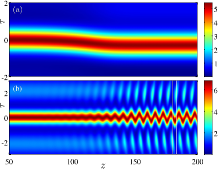
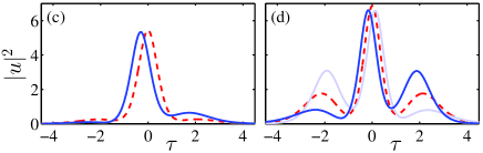
Figure 2: (a), (b) Examples for the density evolution of unstable symmetric states and (c), (d) snapshots for the corresponding states. (a) Evolution of the unstable symmetric state for $X=8$ between the two pitchfork bifurcations $P_{1}$ and $P_{2}$ depicted in Fig. 1. The initial symmetric state, see dashed (red) line in panel (c) evolves towards the asymmetric steady state depicted in solid (blue) in panel (c). (b) Evolution of the unstable symmetric state towards a periodic breathing solution for $X=16$ (i.e., to the right of the Hopf bifurcation point $H$ in Fig. 1). The initial symmetric state [dashed (red) line] and two snapshots of the density for the periodic solution [solid (blue and light blue) lines] separated by half a period, at the times corresponding to the white vertical lines in panel (b), are depicted in panel (d).

It is important to mention that, due to the cavity loss term ($-iu$), the real part of the spectrum is symmetric with respect to Re$(\lambda)=-1$ (see Sec. IV for details). Therefore, tuning the cavity loss parameter is crucial to the existence of the SSB bifurcation as higher values of this parameter shift the real part of the spectrum down precluding the possibility of eigenvalues crossing the origin and leading to such bifurcations. By the same token reducing the value of the cavity loss parameter will induce more eigenvalues to cross the origin and thus leading to richer and more complicated bifurcation scenarios. A detailed analysis of the bifurcations as the cavity loss parameter is varied is outside of the scope of the present manuscript and will be studied in a future work.

III Non-conservative Variational Approximation

III.1 Preliminaries

To employ the NCVA, we consider two sets of dependent variables $u_{1}$ and $u_{2}$. As proposed by Galley and collaborators ref1 ; Galley:14 , these are fixed at an initial time ($z_{i}$), but are not fixed at the final time ($z_{f}$). After applying variational calculus for a non-conservative system, both paths are set equal, $u_{1}=u_{2}$, and identified with the physical path $u$, the so-called physical limit (PL). The action functional for $u_{1}$ and $u_{2}$ is defined as the total action integral of the difference of the Lagrangians between the paths plus the action integral of the functional ${\cal R}$ which describes the generalized non-conservative forces and depends on both paths:

$$S= \int_{z_{i}}^{z_{f}} dz\int_{-\infty}^{\infty}d\tau[\mathcal{L}(u_{1},u_{1,z},u_{1,\tau},\ldots,z)$$

$$-\mathcal{L}(u_{2},u_{2,z},u_{2,\tau},\ldots,z)+\mathcal{R}],$$

where the $z$ and $\tau$ subscripts denote partial derivatives with respect to these variables. The above action defines a new total Lagrangian density:

$$\mathcal{L}_{T}\equiv\mathcal{L}_{1}-\mathcal{L}_{2}+\mathcal{R},$$ (7)

where the first two terms represent the conservative Lagrangian densities for which $\mathcal{L}_{i}\equiv\mathcal{L}(u_{i},u_{i,z},u_{i,\tau},...,z)$, for $i=1,2$, and $\mathcal{R}$ contains all the non-conservative terms. For convenience, $u_{+}=(u_{1}+u_{2})/2$ and $u_{-}=u_{1}-u_{2}$ are defined in such a way that at the physical limit $u_{+}\,\rightarrow\,u$ and $u_{-}\,\rightarrow\,0$. Then, the modified Euler-Lagrange equations for the effective Lagrangian $L=\int_{-\infty}^{\infty}\mathcal{L}_{T}d\tau$ yield

$$\frac{\partial L}{\partial u}-\frac{d}{dt}\left(\frac{\partial L}{\partial\dot{u}}\right)+\int_{-\infty}^{\infty}\left[\frac{\partial\mathcal{R}}{\partial u_{-}}\right]_{\mathrm{PL}}d\tau=0.$$ (8)

Through this method we recover the Euler-Lagrange equation for the conservative terms and all the non-conservative terms are folded into $[\frac{\partial\mathcal{R}}{\partial u_{-}}]_{\mathrm{PL}}$. It is crucial to construct the term $\mathcal{R}$ such that its derivative with respect to the difference variable $u_{-}=u_{1}-u_{2}$ at the physical limit gives back the non-conservative or generalized forces. This part concludes the field-theoretic formulation of the non-conservative problem and so far no approximation has been utilized. The latter will stem from the use of an approximate ansatz for the solutions within the variational method for this extended (to the non-conservative case) Lagrangian formulation.

One key aspect of any variational method is the proper, judicious, choice of ansatz. In this paper, we compare two different ansätze with four and six parameters (i.e., degrees of freedom). We apply the NCVA to Eq. (2) to verify if the reduced dynamical system is able to qualitatively (and quantitatively) capture the SSB instability by following all temporally symmetric and asymmetric solutions to the reduced system of ODEs given by Eq. (8). The conservative Lagrangian density for the NLS, namely Eq. (2) with the right-hand-side equal to zero, is

$$\mathcal{L}=\frac{i}{2}\left(u^{*}u_{z}-uu_{z}^{*}\right)-\left|u_{\tau}\right|^{2}+\frac{1}{2}\left|u\right|^{4}-\Delta\left|u\right|^{2}.$$ (9)

Here, we construct $\left[\partial\mathcal{R}/\partial u_{-}\right]_{\mathrm{PL}}=-iu+iS(\tau)$, by choosing $\mathcal{R}=\left(-iu_{+}+iS(\tau)\right)u_{-}$. Therefore, the relevant non-conservative Lagrangian density can be written as

$$\mathcal{L} = \frac{i}{2}\left(u_{1}^{*}u_{1,z}-u_{1}u_{1,z}^{*}\right)-\left|u_{1,\tau}\right|^{2}+\frac{1}{2}\left|u_{1}\right|^{4}-\Delta\left|u_{1}\right|^{2}$$ (10)

$$- \frac{i}{2}\left(u_{2}^{*}u_{2,z}-u_{2}u_{2,z}^{*}\right)+\left|u_{2,\tau}\right|^{2}-\frac{1}{2}\left|u_{2}\right|^{4}+\Delta\left|u_{2}\right|^{2}$$

$$+ \left(-iu_{+}+iS(\tau)\right)u_{-},$$

where $u_{1}=\left(2u_{+}+u_{-}\right)/2$ and $u_{2}=\left(2u_{+}-u_{-}\right)/2$. For reasons of brevity, we chose to express the Lagrangian density above in 1,2 coordinates. Writing the Lagrangian in $\pm$ coordinates lends itself to lengthier expressions but to more straightforward implementation of the physical limit where the (+) variables directly coincide with the physical variables [and the $(-)$ variables are eliminated]. From $\mathcal{L}$, we can derive, through the Euler-Lagrange equations (8), the full LL model at the PDE level. In order to, however, obtain an analytical insight in the dynamics of the model, our aim is to use an ansatz approximation of the pulse reducing its Lagrangian to a Lagrangian over effective (yet time-dependent) properties of its form, like the amplitude, the width and its center of mass, among others. Then for these effective properties, in the spirit of Refs. JuliaNCVA ; ref4 , a coupled system of ODEs approximating the dynamical evolution will be derived and, perhaps more importantly for our considerations, their corresponding steady states and possible bifurcations will be amenable to analysis.

III.2 Bifurcation Analysis Using the NCVA Approach

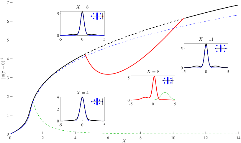
Figure 3: Bifurcation for steady states of the LL model (2) (thick curves) and their approximation using the NCVA methodology with the over-simplified four-parameter ansatz (11) (thin curves) as the pump strength $X$ is varied for $\Delta=0.92$ and $T_{0}=2.3$. Stable (Unstable) branches are depicted with solid (dashed) lines. The (red and green) branches bifurcating from the main branch (blue and black lines) correspond to asymmetric solutions. The insets depict the pulse temporal intensity profiles obtained for $X=4$ (symmetric), $X=8$ (symmetric and asymmetric), and $X=11$ (symmetric) for the original LL model (thick curves) and their NCVA approximation (thin curves). The insets also depict the corresponding stability spectra for these solutions where stable eigenvalues are depicted in blue and unstable eigenvalues in red.

Applying the NCVA methodology described above to the LL model (2) where $\left[\partial\mathcal{R}/\partial u_{-}\right]_{\mathrm{PL}}=-iu+iS(\tau)$, yields $\mathcal{R}=\left(-iu_{+}+iS(\tau)\right)u_{-}$. We first choose the following simple Gaussian ansatz

$$\bar{u}_{j}=a_{j}\exp\left[-\frac{(\tau-\xi_{j})^{2}}{2\sigma_{j}^{2}}\right]\exp(i\,b_{j}),\quad j=1,2$$ (11)

where height $a$, center position $\xi$, width $\sigma$, and phase $b$ are the variational parameters. The ansatz was selected as the simplest localized waveform with freedom to move left or right in order to capture, in the simplest sense, a possible asymmetry in the solution of the original LL model. Applying the NCVA method with this, arguably over-simplified, four-parameter ansatz, leads, through the Euler-Lagrange equations, to a system of algebraic differential equations for which the derivatives of the variational parameters cannot be solved for explicitly. Nonetheless, it is possible to obtain algebraic equations for the corresponding steady state ($\dot{a}=\dot{b}=\dot{\xi}=\dot{\sigma}=0$) solutions of the form:

$$\begin{cases}\frac{a^{2}\sqrt{\pi}}{2\sigma^{2}}+\frac{1}{4}a^{4}\sqrt{2\pi}+\Delta a^{2}\sqrt{\pi}&=\frac{a\sin(b)T_{0}^{2}\beta}{(T_{0}^{2}+2\sigma^{2})},\\[10.00002pt] 2a^{2}\sigma\sqrt{\pi}&=a\cos(b)\sigma\beta,\\[10.00002pt] -\frac{a\sqrt{\pi}}{\sigma}+a^{3}\sqrt{2\pi}\sigma+2\Delta a\sigma\sqrt{\pi}&=\sin(b)\sigma\beta,\\[10.00002pt] 0&=\frac{-a\xi\sin(b)\beta}{\sigma},\end{cases}$$ (12)

where $\beta={2T_{0}\sqrt{2\pi X}}/{\sqrt{T_{0}^{2}+2\sigma^{2}}}$.

Figure 3 depicts the comparison of the bifurcation diagrams for steady state solutions obtained from the original LL model (2) and the NCVA approach for $\Delta=0.92$ and $T_{0}=2.3$ by monitoring $|u(\tau=0)|^{2}$ as a function of pump peak power $X$, in line with the earlier work of Ref. XuCoen . Both solutions for the original LL model and the algebraic NCVA system are obtained by numerical continuation using a standard fixed point iteration (Newton-Krylov). The solutions for the LL model are depicted by the thick curves while the corresponding NCVA approximations by the thin curves. Solid and dashed correspond, respectively, to stable and unstable solutions. The insets in the figure depict pulse temporal intensity profiles $|u|^{2}$ for $X=4$ (symmetric), $X=8$ (symmetric and asymmetric), and $X=11$ (symmetric) for both the LL model (thick curves) and the NCVA reconstructions (thin curves). For completeness, the insets also show the corresponding linearization spectra. As it is evident from the figure, the NCVA with a four-parameter ansatz agrees very well with the symmetric branch of LL model (see black and blue curves). However, for the asymmetric branch there seems to be a large discrepancy between the LL model and its NCVA approximation. In fact, the asymmetric NCVA branch is unstable while it is stable for the original LL model. Upon further inspection (details are omitted for brevity), the instability of the asymmetric NCVA branch stems, instead of a pitchfork bifurcation, from a Hopf bifurcation that creates a stable limit cycle in the variational parameters.

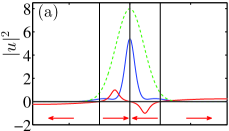
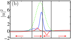
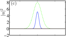
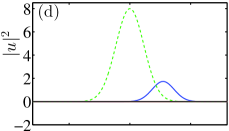
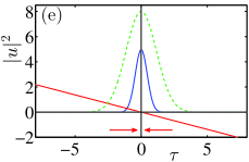
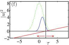
Figure 4: Understanding the importance of including fluid velocity terms in the NCVA ansatz. The different panels depict an overlay of (i) the temporal intensity profile of the pump pulse $|S(\tau)|^{2}$ (green dashed line), (ii) the pulse intensity profile $|u|^{2}$ (blue), and (iii) its corresponding fluid velocity (red, $\times 50$) for (a,b) the LL model (top), (c,d) the four-parameter NCVA (middle), and (e,f) the six-parameter NCVA (bottom) for symmetric $X=8$ (left) and asymmetric $X=8$ (right) steady state solutions. The (red) arrows indicate the direction of the fluid velocity which drives the SSB bifurcation between the symmetric and asymmetric solutions.

It is evident that the four-parameter ansatz is unable to predict the existence of the pitchfork loop of the original LL model and, furthermore, although it is able to predict a SSB bifurcation, it fails to give an accurate estimation for its threshold (i.e., the critical pump power needed to observe asymmetric states). However, this over-simplified ansatz gives two valuable insights regarding how to make a more judicious choice for our ansatz. Firstly, the ansatz (11) has an inherent complication in that its corresponding Euler-Lagrange equations lead to a degenerate system of differential-algebraic equations which can only be explicitly written for the steady state. This degeneracy can be circumvented, as we will show below, by proper balancing of the variational parameters in an ansatz with more degrees of freedom. Secondly, and more importantly, the four-parameter ansatz, by construction, only corresponds to real solutions (up to a global phase shift) that lack a $\tau$-dependence on their phase. This lack of $\tau$-dependence on the phase is responsible for the ansatz solution’s lack of internal flow of the field $u$ along the $\tau$-direction. As we explain below, the asymmetric solution is supported by a delicate balance of the internal flow within this steady state solution. The presence of the underlying flow is clear after careful examination of the (numerically) exact solutions of the original LL model as depicted in panels (a) and (b) of Fig. 4. These panels depict the density (blue) and phase (red) of the solution where the arrows indicate the regions where the fluid velocity, as defined by the gradient of the phase, has different directions. The central density maximum, for both the symmetric and asymmetric solutions, stems from an inward flow towards the center [which corresponds to a sink of flow due to high density through the loss term $iu$ in Eq. (2)] while the “wings”, again for both symmetric and asymmetric solutions, are supported by sources of the underlying flow maintained by the pump. In contrast, the NCVA four-parameter ansatz (11) lacks a phase profile and, therefore, lacks any internal flow as depicted in panels (c) and (d) of Fig. 4. It is then clear that the four-parameter ansatz (11) should be inadequate for capturing the important effects of the underlying current flows of the solutions.

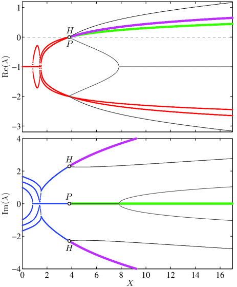
Figure 5: Linearization spectrum for the reduced NCVA ODE (14). The notation is the same as the spectrum for the original LL model depicted in Fig. 1. The reduced ODE model displays a degenerate bifurcation consisting of simultaneous pitchfork (P) and a Hopf (H) bifurcations and thus the asymmetric steady state (see thin black solid lines) is unstable from its inception.

It is important to mention at this stage that steady state solutions (for the density) in NLS-type settings incorporating loss and gain terms must necessarily involve underlying flows that carry “mass” from the gain regions towards the lossy regions. Therefore, in these settings, variational methods should be based on ansätze that incorporate the appropriate underlying current. Inspired by the appreciation of the presence of such underlying flows (and their delicate balance in the steady state solutions) let us choose an ansatz that is capable of supporting such flows. Based on this observation, we introduce a six-parameters ansatz of the form:

$$\bar{u}_{j} = a_{j}\exp\left[\frac{-(\tau-\xi_{j})^{2}}{2\sigma_{j}^{2}}\right]\times$$

$$\exp\left[i(d_{j}(\tau-\xi_{j})^{2}+c_{j}(\tau-\xi_{j})+b_{j})\right],$$

where, in addition to the parameters height $a$, center position $\xi$, width $\sigma$, phase $b$, we have also introduced velocity $c$ and chirp $d$ as variational parameters. Following again the NCVA methodology for this improved ansatz, we obtain the following system of ODEs of the variational parameters:

$$\begin{cases}\dot{a}=&\frac{1}{4}\frac{-4a^{2}\sigma^{3}\sqrt{\pi}+3\sigma^{2}I_{b}-8a^{2}d\sigma^{3}\sqrt{\pi}-2I_{d}}{a\sigma^{3}\sqrt{\pi}},\\[10.00002pt] \dot{b}=&-\frac{1}{8}\frac{8a^{2}\sqrt{\pi}-5a^{4}\sqrt{2}\sqrt{\pi}\sigma^{2}-4I_{\sigma}\sigma^{2}+6I_{a}\sigma a-8a^{2}c^{2}\sqrt{\pi}\sigma^{2}}{a^{2}\sigma^{2}\sqrt{\pi}}\\[10.00002pt] &+\frac{\sigma cI_{c}-a^{2}\Delta\sqrt{\pi}\sigma^{2}}{a^{2}\sigma^{2}\sqrt{\pi}},\\[10.00002pt] \dot{c}=&-\frac{cI_{b}+I_{\xi}}{a^{2}\sigma\sqrt{\pi}},\\[10.00002pt] \dot{d}=&\frac{1}{4}\frac{4a^{2}\sqrt{\pi}-16a^{2}d^{2}\sigma^{4}\sqrt{\pi}-a^{4}\sqrt{2}\sqrt{\pi}\sigma^{2}-4I_{s}\sigma^{2}+2I_{a}\sigma a}{a^{2}\sigma^{4}\sqrt{\pi}},\\[10.00002pt] \dot{\sigma}=&-\frac{1}{2}\frac{\sigma^{2}I_{b}-8a^{2}d\sigma^{3}\sqrt{\pi}-2I_{d}}{a^{2}\sigma^{2}\sqrt{\pi}},\\[10.00002pt] \dot{\xi}=&\frac{2a^{2}\sigma c\sqrt{\pi}+I_{c}}{a^{2}\sigma\sqrt{\pi}},\end{cases}$$ (14)

where the over-dot denotes derivative with respect to $z$. Although it is possible to explicitly solve for the derivatives of the variational parameters, the resulting NCVA ODEs are cumbersome in that they include the terms $I_{a},I_{b},I_{c},I_{d},I_{\xi},$ and $I_{\sigma}$ which involve integrals that cannot be explicitly evaluated:

$$\begin{cases}I_{a}=&\displaystyle\int_{-\infty}^{\infty}E\sin(\Phi)\,d\tau,\\[8.61108pt] I_{b}=&\displaystyle\int_{-\infty}^{\infty}aE\cos(\Phi)\,d\tau,\\[8.61108pt] I_{c}=&\displaystyle\int_{-\infty}^{\infty}aE(\tau-\xi)\cos(\Phi)\,d\tau,\\[8.61108pt] I_{d}=&\displaystyle\int_{-\infty}^{\infty}aE(\tau-\xi)^{2}\cos(\Phi)\,d\tau,\\[8.61108pt] I_{\sigma}=&\displaystyle\int_{-\infty}^{\infty}\frac{aE}{\sigma^{3}}\sin(\Phi)\,d\tau,\\[8.61108pt] I_{\xi}=&\displaystyle\int_{-\infty}^{\infty}\Big{[}aE\left(-2d(\tau-\xi)-c\right)\cos(\Phi)\\[10.00002pt] &\displaystyle\quad\quad+\frac{aE(\tau-\xi)}{\sigma^{2}}\sin(\Phi)\Big{]}\,d\tau,\end{cases}$$

where $\Phi=d(\tau-\xi)^{2}+c(\tau-\xi)+b$ and $E=2\sqrt{X}e^{-\frac{(\tau-\xi)^{2}}{2\sigma^{2}}}e^{-\frac{\tau^{2}}{T_{0}^{2}}}$. Nonetheless, for our numerical studies it suffices to evaluate numerically these integrals as we seek stationary states or as we follow the dynamics of the parameters as $z$ changes.

Figure 6: Bifurcation diagram as in Fig. 3 but for the more complete six-parameter ansatz (III.2). Same layout and meaning as in Fig. 3.

Figure 5 depicts the linearization spectrum for the reduced NCVA six-parameter ODE model (14) that should be compared to the linearization spectrum of original LL model depicted in Fig. 1. It is clear that both spectra share some of the bifurcation structure but, at the same time, they have notable differences. For instance, although the reduced NCVA ODE is able to capture the SSB at $X\approx 3.8$, reasonably close to the actual bifurcation of the original model at $X\approx 4.6$, the bifurcation, instead of being a pitchfork one, is a degenerate one comprising simultaneous pitchfork and Hopf bifurcations. This is the reason why the reduced ODE NCVA model transitions directly from a stable symmetric solution to a stable (asymmetric) limit cycle instead of a stable asymmetric steady state as in the original LL model. The bifurcation diagram for the six-parameter ansatz (III.2), together with the one from the original LL model, is depicted in Fig. 6 using the same layout as Fig. 3. As it is clear for comparing Figs. 3 and 6, the six-parameter ansatz does a much better job at capturing the asymmetry states (see insets) and the threshold for the primary SSB bifurcation than its four-parameter counterpart. However, as we noted above (and similar to the case of the reduced four-parameter NCVA ode) the bifurcation predicted by the NCVA ODEs (14) produces an unstable asymmetric state and a stable (asymmetric) limit cycle. Nonetheless, the six-parameter ansatz is now able to capture the essence of the underlying flow as it can be seen from panels (e) and (f) of Fig. 4. Furthermore, and perhaps more importantly, the improved six-parameter NCVA approach is also able to predict reasonably well the threshold for the pump power for the onset of the SSB bifurcation. The fact that the NCVA method is insufficient in characterizing the details of the SSB instability is, arguably, the consequence of employing ansätze that (while remaining tractable) lack the proper freedom to include underlying flows that are akin to the solutions displayed by the original LL model. For instance, in order to capture the details of the underlying flows depicted in panels (a) and (b) of Fig. 4 it should be necessary to include a fluid flow that has, at least, three zeros and that would entail, if using polynomials as a basis for expanding the phase, a quartic polynomial (i.e., five parameters) for the phase. Such an ansatz would require five phase variational parameters and five shape (density) parameters leading to a cumbersome system of ten couple ODEs. Such a venture falls outside of the scope of the present manuscript.

IV Local Bifurcation Analysis

In this section, we employ a complementary, dynamical systems inspired approach based on a center manifold reduction to determine the dynamics of the system close to the pitchfork bifurcations.

IV.1 Reduced equation

Let us consider Eq. (1) with, as before, $\eta=-1$. In this approach it is more convenient to work with real variables. We therefore set

$$E=U+iV,$$ (15)

where $U$ and $V$ are real-valued functions, and then Eq. (1) is equivalent to the system

$$\begin{cases}U_{z}=-U-V_{\tau\tau}+\Delta V-(U^{2}+V^{2})V+S(\tau),\\[4.30554pt] V_{z}=-V+U_{\tau\tau}-\Delta U+(U^{2}+V^{2})U.\end{cases}$$ (16)

The numerical computations in Fig. 6 show the existence of a branch of symmetric steady state solutions for values of $X$ between 0 and 14, which can be continued to large $X$. Using the implicit function theorem, one can prove the existence and uniqueness of this branch for small values of $X$, together with the fact that a solution $(U_{X}(\tau),V_{X}(\tau))$ is smooth and decays exponentially to $0$, as $|\tau|\to\infty$. Moreover, one can show that there are no bifurcations, for $X$ sufficiently small. Here, we are interested in the two pitchfork bifurcations predicted by the previous numerical computations at $X_{1}$ = 4.596695 and $X_{2}$ = 10.604008.

Consider a symmetric steady solution $(U_{X},V_{X})$ on the branch in Fig. 6. By setting

$$U=U_{X}+\nu,\quad\quad V=V_{X}+v.$$ (17)

where $\nu$ and $v$ describe the deviations from this steady solution, we obtain the new system:

$$w_{z}=\mathcal{A}_{X}w+\mathcal{J}(\mathcal{R}_{2}(w,w)+\mathcal{R}_{3}(w)),$$ (18)

in which $w=(\nu,v)^{T}$ and $\mathcal{A}_{X}$ is the matrix linear operator

$$\mathcal{A}_{X}=-\mathbb{I}+\mathcal{J}\mathcal{L}_{X},$$ (19)

where $\mathbb{I}$ is the identity matrix,

$$\mathcal{J}=\begin{pmatrix}0&-1\\ 1&0\end{pmatrix},$$

and $\mathcal{L}_{X}$ is the linear operator defined by

$$\mathcal{L}_{X}=\begin{pmatrix}\partial^{2}_{\tau}-\Delta+3U_{X}^{2}+V_{X}^{2}&2U_{X}V_{X}\\ 2U_{X}V_{X}&\partial^{2}_{\tau}-\Delta+U_{X}^{2}+3V_{X}^{2}\end{pmatrix}.$$

Finally, $\mathcal{R}_{2}(w_{1},w_{2})$ is the bilinear map given by

$$\mathcal{R}_{2}(w_{1},w_{2})=\begin{pmatrix}3U_{X}\nu_{1}\nu_{2}+V_{X}(\nu_{1}v_{2}+\nu_{2}v_{1})+U_{X}v_{1}v_{2}\\ V_{X}\nu_{1}\nu_{2}+U_{X}(\nu_{1}v_{2}+\nu_{2}v_{1})+3V_{X}v_{1}v_{2}\end{pmatrix},$$

for $w_{1}=(\nu_{1},v_{1})^{T}$ and $w_{2}=(\nu_{2},v_{2})^{T}$, and $\mathcal{R}_{3}(w)$ is the cubic map given by

$$\mathcal{R}_{3}(w)=\begin{pmatrix}(\nu^{2}+v^{2})\nu\\ (\nu^{2}+v^{2})v\end{pmatrix},$$

for $w=(\nu,v)^{T}$. We regard Eq. (18) as an infinite-dimensional dynamical system in the phase space $H=L^{2}(\mathbb{R})\times L^{2}(\mathbb{R})$ equipped with the usual scalar product

$$\langle w_{1},w_{2}\rangle=\int_{\mathbb{R}}(\nu_{1}(\tau)\nu_{2}(\tau)+v_{1}(\tau)v_{2}(\tau))d\tau.$$

In this Hilbert space, $\mathcal{A}_{X}$ is a closed linear operator with domain $H^{2}(\mathbb{R})\times H^{2}(\mathbb{R})$, and the operators $\mathcal{J}$ and $\mathcal{L}_{X}$ are skew- and self-adjoint, respectively. The nonlinear terms $\mathcal{R}_{2}$ and $\mathcal{R}_{3}$ are smooth maps.

Varying the parameter $X$ in Eq. (18), the bifurcation points are the values of $X$ where the structure of the purely imaginary part of the spectrum of the linear operator $\mathcal{A}_{X}$ changes. Notice that the spectrum of $\mathcal{A}_{X}$ is symmetric with respect to the vertical line Re$(\lambda)=-1$ in the complex plane. Indeed, since $\mathcal{J}$ and $\mathcal{L}_{X}$ are skew- and self-adjoint operators, respectively, the spectrum of $\mathcal{J}\mathcal{L}_{X}$ is symmetric with respect to the imaginary axis, so that the spectrum of $\mathcal{A}_{X}=-\mathbb{I}+\mathcal{J}\mathcal{L}_{X}$ is symmetric with respect to the vertical line Re$(\lambda)=-1$ in the complex plane. Moreover, it is also symmetric with respect to the real axis, since $\mathcal{A}_{X}$ is a real operator. These two properties are clearly satisfied by the numerically obtained spectrum depicted in Fig. 1.

The essential spectrum of $\mathcal{A}_{X}$ can be determined analytically. Since $\mathcal{A}_{X}$ is a differential operator with asymptotically constant coefficients, its essential spectrum coincides with the spectrum of the asymptotic operator $\mathcal{A}_{0}$ which has constant coefficients. Then a standard Fourier analysis allows to compute explicitly the spectrum of $\mathcal{A}_{0}$, and conclude that the essential spectrum of $\mathcal{A}_{X}$ is the set

$$\sigma_{\rm ess}=\{-1\pm i(k^{2}+\Delta),\;k\in\mathbb{R}\},$$

which lies entirely in the open left half complex plane. Consequently, bifurcations can only arise due to point spectrum, which consists of eigenvalues with finite algebraic multiplicities. For sufficiently small $X$, standard perturbation arguments show that the spectrum of $\mathcal{A}_{X}$ stays close to the one of $\mathcal{A}_{0}$. In particular, it lies in the left half complex plane, and no bifurcations/instabilities occur for small $X$. The previous numerical computations show that there exists a first value $X_{1}$ at which one (simple) eigenvalue crosses the origin and becomes positive for $X>X_{1}$ (see point $P_{1}$ in Fig. 1). All other eigenvalues have negative real parts. Increasing $X$, there is a second value $X_{2}$ where this simple eigenvalue crosses the origin back in the left half complex plane (see point $P_{2}$ in Fig. 1). Our purpose is to study the two (pitchfork) bifurcations which occur at these parameter values, and which are directly related to the SSB phenomena observed experimentally in Ref. XuCoen .

We denote by $\lambda_{0}(X)$ the simple eigenvalue above, so that we have

$$\sigma(\mathcal{A}_{X})=\{\lambda_{0}(X)\}\cup\sigma_{-}(\mathcal{A}_{X}),$$ (20)

$$\quad\sigma_{-}(\mathcal{A}_{X})\subset\{\lambda\in\mathbb{C}\,;\,\mathrm{Re}(\lambda)\leqslant-\gamma\},$$ (21)

for some $\gamma>0$, and

$$\lambda_{0}(X)<0\;\mbox{ for }\;X<X_{1},$$ (22)

$$\lambda_{0}(X_{1})=0,$$

$$\lambda_{0}(X)>0\;\mbox{ for }\;X_{1}<X<X_{2},$$

$$\lambda_{0}(X_{2})=0.$$

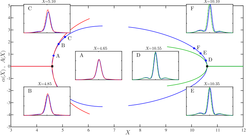
Figure 7: Steady state comparison between the original LL model (2) and the center manifold approach (see text) close to the pitchfork bifurcation points. The figure depicts the coefficients determining the amount of asymmetry for the LL model as monitored by $\alpha(X)$, defined in Eq. (29), (see blue curves containing the points A, B, C, D, E, and F) and for the center manifold approach by $A(X)$ (see red [about bifurcation point $X_{1}$] and green [about bifurcation point $X_{2}$] curves). The insets correspond to the steady state asymmetric solutions for both the LL model (solid curves) and the center manifold approach (dashed curves) at the points A, B, C, D, E, and F indicated in the bifurcating branches corresponding, respectively, to pump powers $X$ = 4.65, 4.85, 5.1, 10.55, 10.35, and 10.1.

The following arguments work for both bifurcation points $X_{1}$ and $X_{2}$. Choose one of these values and denote it by $X_{*}$. We set

$$\mathcal{A}_{*}=\mathcal{A}_{X_{*}},\quad\mathcal{L}_{*}=\mathcal{L}_{X_{*}},\quad{\rm and}\quad\mathcal{R}_{*,2}=\mathcal{R}_{X_{*},2}.$$

Further, we consider an eigenvector $\zeta_{*}$ in the one-dimensional kernel of $\mathcal{A}_{*}$ and an eigenvector $\zeta_{*}^{*}$ in the one-dimensional kernel of the adjoint operator $(\mathcal{A}_{*})^{*}$. We claim that we can choose $\zeta_{*}^{*}$ such that

$$\zeta_{*}^{*}=\mathcal{J}\zeta_{2}\;\mbox{~{}and~{}}\;\mathcal{A}_{*}\zeta_{2}=-2\zeta_{2}.$$

Indeed, since $\mathcal{J}$ and $\mathcal{L}_{X}$ are skew- and self-adjoint operators, respectively, we find

$$(\mathcal{A}_{*})^{*}\zeta_{*}^{*}=0\, \Leftrightarrow\,-(\mathcal{L}_{*}\mathcal{J})\zeta_{*}^{*}=\zeta_{*}^{*},$$ (23)

$$\Leftrightarrow\,\mathcal{A}_{*}(\mathcal{J}\zeta_{*}^{*})=-2(\mathcal{J}\zeta_{*}^{*}).$$

The last equality shows that $\mathcal{J}\zeta_{*}^{*}$ is an eigenvector of $\mathcal{A}_{*}$ associated to the eigenvalue $-2$ [the symmetric of 0 with respect to the vertical line Re$(\lambda)=-1$], and proves the claim.

The analytical and numerical computations of the essential and point spectra, respectively, above show that $\mathcal{A}_{*}$ has precisely one simple eigenvalue on the imaginary axis [located at the origin], and that the remaining spectrum lies entirely in the open left half complex plane. By arguing with the center manifold theorem, e.g., see (MH-Iooss, , Chapter 2), we conclude that the dynamical system (18) possesses a one-dimensional center manifold, for any $X$ close to $X_{*}$. All bounded solutions of Eq. (18) lie on this manifold and are of the form

$$w(z)=A(z)\zeta_{*}+\Phi(A(z),X),$$ (24)

in which $A$ is a real-valued function and $\Phi$, depending upon $A$ and the parameter $X$, satisfies

$$\Phi(A,X)=\mathcal{O}(|A|(|X-X_{*}|+|A|),$$

for small $A$ and $X$ close to $X_{*}$, and the orthogonality condition

$$\langle\Phi(A,X),\zeta_{*}^{*}\rangle=0.$$ (25)

Here, $\zeta_{*}$ and $\zeta_{*}^{*}$ are the eigenvectors in the kernels of the operator $\mathcal{A}_{*}$ and its adjoint operator, respectively. The dynamics of the center manifold is determined by a scalar ODE

$$\frac{dA}{dz}=f(A,X).$$ (26)

Our purpose is to compute the leading order terms in the expansion of the reduced scalar field $f$. Notice that the system (18) is invariant under the reflection $\tau\mapsto-\tau$. As a consequence, $f$ is odd in $A$,

$$f(A,X)=-f(-A,X),$$

so that its Taylor expansion is of the form

$$f(A,X)=c_{0}(X)A+c_{3}A^{3}+\mathcal{O}(|A|^{3}(|X-X_{*}|+A^{2})),$$

in which $c_{0}(X)$ and $c_{3}$ are real constants. Since the (single) eigenvalue of the linearization at $0$ of the reduced scalar field $f$ is precisely $\lambda_{0}(X)$, we conclude that

$$c_{0}(X)=\lambda_{0}(X),$$

In particular $c_{0}(X_{*})=0$ and its values for $X$ close to $X_{*}$ are given by the previous numerical calculations (see Sec. II). Next, in order to compute $c_{3}$, we set $X=X_{*}$ and replace the ansatz (24) into the system (18). Taking into account Eq. (26), the expansion of $f$, and expanding the reduction function $\Phi(A,X)$ at $X=X_{*}$,

$$\Phi(A,X_{*})=\Phi_{0}A+\Phi_{2}A^{2}+\Phi_{3}A^{3}+\mathcal{O}(|A|^{4}),$$

we obtain the equality

$$\mathcal{A}_{*}\Phi_{2}=-\mathcal{J}R_{*,2}(\zeta_{*},\zeta_{*}).$$ (27)

The orthogonality condition Eq. (25) determines uniquely $\Phi_{2}$, and as a consequence of the reflection symmetry $\tau\mapsto-\tau$ of Eq. (18), we have that $\Phi_{2}$ is an even function. In particular, $\Phi_{2}$ is the unique even solution of the equation. Next, at $\mathcal{O}(A^{3})$, we obtain:

$$c_{3}\zeta_{*}=\mathcal{A}_{*}\Phi_{3}+2\mathcal{J}\mathcal{R}_{*,2}(\zeta_{*},\Phi_{2})+\mathcal{J}\mathcal{R}_{3}(\zeta_{*}).$$

Taking the scalar product with $\zeta_{*}^{*}=\mathcal{J}\zeta_{2}$, and using the fact that $\zeta_{*}^{*}$ belongs to the kernel of the adjoint of $\mathcal{A}_{*}$, we obtain the second coefficient

$$c_{3}=\frac{1}{\langle\zeta_{*},\mathcal{J}\zeta_{2}\rangle}\left(\langle 2\mathcal{R}_{*,2}(\zeta_{*},\Phi_{2}),\zeta_{2}\rangle+\langle\mathcal{R}_{3}(\zeta_{*}),\zeta_{2}\rangle\right).$$

IV.2 Local dynamics

The local dynamics on the one-dimensional center manifold is qualitatively given by the signs of the two coefficients $c_{0}(X)$ and $c_{3}$. These coefficients are computed numerically, and the result confirms the situation depicted in Fig. 6. The sign of $c_{0}(X)$ is the same as the one of $\lambda_{0}(X)$ [see Eq. 22], and

$$c_{3}<0,\;\mbox{~{}for~{}}\;X=X_{1},\mbox{~{}and~{}}\;c_{3}>0,\;\mbox{~{}for~{}}\;X=X_{2}.$$ (28)

At both bifurcation points $X_{1}$ and $X_{2}$, we are in the presence of a pitchfork bifurcation in which a pair of asymmetric stable equilibria appears from or disappears into the symmetric equilibrium which, in turn, changes its stability. Moreover, there is a pair of heteroclinic orbits connecting the unstable symmetric equilibrium at $z=-\infty$ with the stable asymmetric equilibria at $z=\infty$. These solutions persist for the full system, and can be computed as solutions of Eq. (1) going back through the reduction procedure, successively from the formulas (24), (17), and (15). In particular, the heteroclinic connection describes the transition dynamics from the unstable symmetric to the stable asymmetric solution.

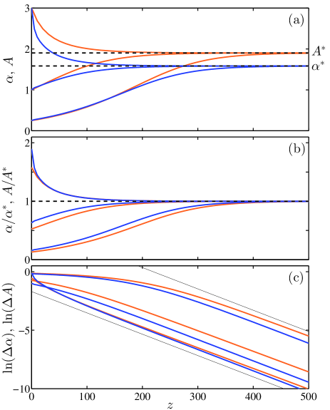
Figure 8: Orbits representing the dynamics settling to the asymmetric steady states past the first pitchfork bifurcation point. Depicted is the evolution for the asymmetry coefficients $\alpha(z)$ and $A(z)$ (see text) for a pump strength is $X=4.85$ that is to the right of the first pitchfork bifurcation point $X_{1}=4.596695$. The blue (dark) curves correspond to the original model ($\alpha(z)$) while the orange (gray) curves correspond to the reduced equation ($A(z)$). The orbits tend towards their corresponding steady state solutions $\alpha^{*}$ and $A^{*}$ which correspond to the stable asymmetric state created by the pitchfork bifurcation. Panel (b) corresponds to panel (a) by normalizing the $A(z)$ and $\alpha(z)$ orbits by their respective steady states. Panel (c) shows the logarithm of the normalized distance to the steady state $\Delta\alpha=(\alpha-\alpha^{*})/\alpha^{*}$ and $\Delta A=(A-A^{*})/A^{*}$. In this panel we also depict with thin (black) lines the slope $\lambda(4.85)=-0.01824$ corresponding to the stability eigenvalue of the asymmetric state [see small black dot next to the point $P_{1}$ on the thin (black) branch depicted in the top panel of Fig. 1] which is shown to coincide with the rate of attraction towards the asymmetric steady state for both the original model and the reduced equation.

Based on the bifurcation analysis above, we compare the solutions (24) given by the center manifold approach to ones found directly from the original LL model (1) for $\eta=-1$, $\Delta=0.92$, and $T_{0}=2.3$. In particular, we compare the asymmetric stationary states described by Eqs. (17) and (24) with the ones obtained from the LL (2) by projecting the numerically found steady state solutions of the latter along the symmetric and asymmetric branches for values of $X$ near the bifurcation points $X_{1}$ and $X_{2}$. Therefore, the asymmetric solutions of Eq. (2) are fit using the symmetric solutions plus $\alpha$ times the eigenvector of the translation mode, i.e. the eigenvector $\zeta_{*}$ associated with the bifurcation point $X_{*}$ [see Eq. (4) and Fig. 1], but now written in original complex variables associated with $u(z,\tau)$.

Therefore, we find the best (in the least-squares sense) scalar value $\alpha$ such that:

$$u_{\mathrm{Asym}}(X_{*}+\delta X)\approx u_{\mathrm{Sym}}(X_{*}+\delta X)+\alpha(X_{*}+\delta X)\,\zeta_{*}.$$ (29)

By using a nonlinear least-square solver, we extract the value of $\alpha(X)$ around each bifurcation point $X_{1}$ and $X_{2}$ and compare it with the value of $A(X)$ from the reduced equation. Fig. 7 depicts a plot of $A(X)$ and $\alpha(X)$ close to both pitchfork bifurcations. As the figure shows, the shape of the bifurcation is well captured by the center manifold approach. In fact, as expected, the reduced equation correctly captures the concavity of the bifurcating branch at both bifurcation points. In the figure, the insets depict the steady state profile comparison between the original model and the center manifold approach for values of the pump power $\delta X$ = 0.05, 0.25, and 0.5 units away from both bifurcation points. As it is clear from the insets, the center manifold approach approximates very well the shape of the steady state solutions particularly close to the bifurcation points. Therefore, the reduced equation provides a very good agreement for the statics, i.e. steady states, of the original model close to the bifurcation points.

We now focus on the dynamics close to the bifurcation. In particular, let us study how solutions, starting from a perturbed (unstable) symmetric solution, evolve towards the (stable) asymmetric steady [an example portraying this evolution is depicted in Fig. 2(a)]. Figure 8(a) depicts the dynamical evolution of the asymmetry coefficients $A$ and $\alpha$, as defined above, for initial conditions above and below the corresponding steady state solutions $A^{*}$ and $\alpha^{*}$ for a value of $X$ past the first pitchfork bifurcation point. As the figure shows, both the original LL dynamics and the center manifold reduction produce orbits that settle towards their corresponding (stable) asymmetric steady states. In order to better compare the decay in both systems, we depict in Fig. 8(b) the orbits normalized by their corresponding steady states. Finally in Fig. 8(c) we depict the logarithm of the distance to the corresponding steady states. As it is clear from this panel, the steady state is reached exponentially fast with a rate that precisely coincides with the stability eigenvalue for the asymmetric state [see small black dot next to the point $P_{1}$ on the thin (black) branch depicted in the top panel of Fig. 1] as suggested by the thin black (dark) lines depicting the rate using $\lambda(4.85)=-0.01824$. The figure confirms that the center manifold approach is not only capable of reproducing the right statics for the asymmetric branches, but it is also capable of reproducing the main qualitative features of the dynamics as the solutions settle towards the stable asymmetric states.

V Conclusions & Future Challenges

In this paper we considered different theoretical techniques aiming at a more detailed analytical and numerical understanding of the phenomenology arising in a coherently-driven passive optical Kerr resonator, experimentally observed in Ref. XuCoen and modelled by the Lugiato-Lefever equation (LL) LL that corresponds to a non-Hamiltonian variant of the nonlinear Schrödinger equation. In particular, we applied both a non-conservative variational approximation (NCVA) of Ref. JuliaNCVA and a center manifold technique to study the spontaneous symmetry breaking (SSB) bifurcations arising in this system. It is found that variational ansätze lacking the appropriate phase variation are not able to capture the intrinsic underlying velocity fields and the delicate balance present in the steady state density solution. These flows are ubiquitous in systems with gain and loss as the steady state consists of a balance between regions with gain and loss provided by flows from the former regions (sources) to the latter ones (sinks). Using a suitably adjusted variational ansatz, including higher order phase terms while remaining tractable, the NCVA is capable of accurately predicting the threshold in the pump power for the onset of SSB —although it is not adequate for fully capturing the complex bifurcation structure (especially so at large pumping strength/large nonlinearity). To obtain a more complete and quantitative, as well as mathematically a more rigorously justifiable description, we have then employed a center manifold approach capable of capturing both the forward and reverse pitchfork bifurcations of the original system in terms of the corresponding locations and profile shapes of the steady states and also in terms of the rate of convergence towards the stable asymmetric state when the symmetric one is rendered unstable. The numerical determination of the linearization spectrum of the system was not only important for completing the calculations associated with the center manifold method; it was also crucial towards a detailed understanding of the full stability/instability transitions.

In that same vein, the identification of the parametric dependence of the spectrum has enabled us to uncover the emergence in the original LL model of a (potentially quite relevant to experiments in this system) Hopf bifurcation. This, in turn, was dynamically found to give rise to stable periodic solutions and hence illustrate that more complex bifurcation scenaria may arise as the cavity loss parameter is varied.

It should be interesting to study in more detail these more complex bifurcation and SSB scenaria and their implications for the original physical system. In that regard, it may be beneficial to explore the possibility to identify these periodic orbits as exact solutions of the numerical LL problem past the Hopf bifurcation point that we have identified here, via a fixed point iteration at the Poincaré recurrence of the relevant periodic orbit, or using the center manifold technique. Moreover, this would enable to explore the stability (Floquet multipliers) associated with this orbit. Another natural direction would be to consider similar LL models in two-dimensional settings (even if these may be less relevant from an experimental perspective in nonlinear optics) in order to appreciate how SSB phenomena may interplay with external drives and also with the potential of such higher dimensional models to feature collapse. Lastly, from the point of view of more recent experiments in connection to the LL equation, a deeper understanding of the dynamics and interactions, as well as the trapping and manipulation of temporal cavity solitons (and corresponding effective “particle” descriptions thereof) may be relevant to pursue tweezing ; patterns .

References

References

- (1) H. Arodz, J. Dziarmaga, W. H. Zurek, Patterns of symmetry breaking, Kluwer Academic Publishers (Dordrech, 2003).
- (2) H. E. Stanley, Introduction to phase transitions and critical phenomena, Oxford University Press (Oxford, 1971).
- (3) V. M. Kenkre and D. K. Campbell Phys. Rev. B 34, 4959(R) (1986).
- (4) B. V. Gisin, A. Kaplan, and B. A. Malomed, Phys. Rev. E 62, 2804 (2000).
- (5) B. Maes, M. Soljačoć, J. D. Joannopoulos P. Bienstman, R. Baets, S-P. Gorza, and M. Haelterman, Switching through symmetry breaking in coupled nonlinear micro-cavities Opt. Express 14, 10678 (2006).
- (6) P. G. Kevrekidis, Z. Chen, B. A. Malomed, D. J. Frantzeskaki, and M. I. Weinstein. Phys. Lett. A 6, 275–280 (2005).
- (7) B. A. Malomed, “Spontaneous Symmetry Breaking, Self-Trapping, and Josephson Oscillations”, Progress in Optical Science and Photonics, Springer-Verlag, Berlin, vol. 1 (2013).
- (8) S. V. Suchkov, A. A. Sukhorukov, J. Huang, S. V. Dmitriev, C. Lee, Yu. S. Kivshar, arXiv:1509.03378.
- (9) V. V. Konotop, J. Yang, D. A. Zezyulin, arXiv:1603.06826.
- (10) H. Cartarius and G. Wunner Phys. Rev. A 86, 013612 (2012); see also: A.S. Rodrigues, K. Li, V. Achilleos, P.G. Kevrekidis, D.J. Frantzeskakis, C.M. Bender, Rom. Rep. Phys. 65, 5 (2013).
- (11) V. Achilleos, P. G. Kevrekidis, D. J. Frantzeskakis, and R. Carretero-González. Phys. Rev. A 86 013808 (2012).
- (12) V. Achilleos, P.G. Kevrekidis, D.J. Frantzeskakis, and R. Carretero-González, Localized Excitations in Nonlinear Complex Systems, Nonlinear Systems and Complexity 7 3–42 (2014).
- (13) Y. Xu and S. Coen, Opt. Lett. 39, 3492 (2014).
- (14) L. A. Lugiato and R. Lefever, Spatial dissipative structures in passive optical systems. Phys. Rev. Lett. 58, 2209–2211 (1987).
- (15) M. Haelterman, S. Trillo, and S. Wabnitz, Dissipative modulation instability in a nonlinear dispersive ring cavity. Opt. Commun. 91, 401–407 (1992).
- (16) F. Leo, S. Coen, P. Kockaert, S.-P. Gorza, Ph. Emplit, and M. Haelterman, Nat. Photon. 4, 471–476 (2010).
- (17) J. K. Jang, M. Erkintalo, S. G. Murdoch, and S. Coen, Nat. Photon. 7, 657 (2013).
- (18) J. Rossi, R. Carretero-González, and P. G. Kevrekidis, Non-Conservative Variational Approximation for Nonlinear Schrödinger Equations. arXiv:1508.07040.
- (19) M. Haragus and G. Iooss, “Local bifurcations, center manifolds, and normal forms in infinite dimensional dynamical systems”, Universitext, Springer-Verlag, EDP Sciences (2011).
- (20) C. Godey, I. Balakireva, A. Coillet, and Y. K. Chembo, Phy. Rev. A 89, 063814 (2014).
- (21) C. R. Galley, Phys. Rev. Lett. 110, 174301 (2013).
- (22) P. G. Kevrekidis, Phys. Rev. A 89, 010102R (2014).
- (23) C. R. Galley, D. Tsang, L. C. Stein, The principle of stationary nonconservative action for classical mechanics and field theories, arXiv:1412.3082 [math-ph].
- (24) J. K. Jang, M. Erkintalo, S. Coen, S. G. Murdoch Nature Communications 6, 7370 (2015).
- (25) P. Parra-Rivas, D. Gomila, M. A. Matias, S. Coen, L. Gelens, Phys. Rev. A 89, 043813 (2014).