Kinetic Transition Networks for the Thomson Problem and Smale’s 7th Problem

Abstract

The Thomson Problem, arrangement of identical charges on the surface of a sphere, has found many applications in physics, chemistry and biology. Here we show that the energy landscape of the Thomson Problem for $N$ particles with $N=132,\ 135,\ 138,\ 141,\ 144,\ 147,$ and 150 is single funnelled, characteristic of a structure-seeking organisation where the global minimum is easily accessible. Algorithmically constructing starting points close to the global minimum of such a potential with spherical constraints is one of Smale’s 18 unsolved problems in mathematics for the 21st century because it is important in the solution of univariate and bivariate random polynomial equations. By analysing the kinetic transition networks, we show that a randomly chosen minimum is in fact always ‘close’ to the global minimum in terms of the number of transition states that separate them, a characteristic of small world networks.

I Introduction

The Thomson Problem is an important model in both physics and chemistry and is easily stated: find the minimum energy of a system composed of $N$ identical charges that are constrained to move on the surface of a sphere of unit radius, i.e. minimise the potential energy function

$$V_{\mbox{Th}}(\textbf{r})=\sum_{1\leq i<j\leq N}\frac{1}{r_{ij}},$$ (1)

where $r_{ij}=\sqrt{(x_{i}-x_{j})^{2}+(y_{i}-y_{j})^{2}+(z_{i}-z_{j})^{2}}$, subject to spherical constraints $x_{i}^{2}+y_{i}^{2}+z_{i}^{2}=1$ for all $i=1,\dots,N$.

The model was proposed by J. J. Thomson as a representation of atomic structure thomson1904xxiv , although it was soon abandoned in this context. However, it has subsequently found many applications in physics, chemistry and biophysics because it captures the competition between local order for neighbouring particles and long-range constraints due to the curvature and geometry. In particular, it is not generally possible to arrange every particle in an identical environment. The resulting model can provide insight into the forces governing far more complex systems, such as the arrangement of proteins in shells of spherical viruses caspar1962physical ; marzec1993pattern ; bruinsma2003viral ; zandi2004origin , fullerene patterns for carbon clusters kroto1985c , the surface ordering of liquid metal drops confined in Pauli traps davis1997history , and the behaviour of colloidal particles trapped at a fluid-fluid interface disc03 ; LipowskyBMNB05 ; EinertLSBB05 ; Kusumaatmaja2013 ; meng2014elastic ; IrvineVC10 ; IrvineBC12 ; PhysRevE.88.012405 .

In the mathematics and computer science communities, the Thomson Problem has gained special attention because it appears in the 7th problem in Steven Smale’s list of eighteen unsolved problems for the 21st century smale1998mathematical ; smale1998mathematical-2 . The problem as posed by Smale requires us to algorithmically blum2012complexity construct a collection of starting points, say $\textbf{r}^{*}$, so that for a given number of particles $N$, $V_{\mbox{Th}}(\textbf{r}^{*})-V_{\mbox{Th}}(\textbf{r}_{\mbox{gm}})\leq\mbox{const}\times\log N$, for $N\geq 2$. Here, $\textbf{r}_{\rm gm}$ is the global minimum for the given $N$.

Constructing such points corresponds to finding a good starting system of polynomial equations to locate all the complex solutions for sets of polynomial equations and to realise the Fundamental Theorem of Algebra shub1993complexity ; armentano2011minimizing .

Given its broad relevance, the global minimum of the Thomson Problem has been studied extensively siman86 ; ErberH91 ; constrained ; ErberH95 ; altschuler97 ; ErberH97 ; genetic ; altschuler05 ; AltschulerP06 ; WalesU06 ; WalesMA09 ; brauchart2009riesz ; brauchart2012next ; Bowick . Analytical solutions are known for $N=2-6$ and $12$ andreev1996extremal ; schwartz20105 . For $N=4,6$ and $12$, they correspond to Platonic solids. The global minimum structures for larger $N$ have been tackled computationally saff1997distributing ; kuijlaars1998asymptotics ; disloc99 ; livshits99 ; BowickNT00 ; BowickCNT02 ; BowickCNT06 ; AltschulerP06 ; WalesU06 ; PhysRevE.78.010601 ; lafave2014discrete . Most of these studies, however, only focus on the global minima. In the present work we search extensively for (most, if not all) the minima and transition states of the Thomson Problem at some selected sizes up to $N=150$, and study the networks defined by these minima and the transition states that connect them. Using disconnectivity graphs beckerk97 ; walesmw98 , we find that the Thomson Problem exhibits a single funnel for all $N$ considered. We also show that the networks exhibit typical characteristics of a small world network. Hence, in the context of Smale’s 7th problem, all minima are only a few steps from the global minimum.

II Potential Energy Landscapes of the Thomson Problem

We begin by collecting some basic definitions: a local minimum of a potential is a point in the configuration space where the gradient vanishes and at which the Hessian matrix has no negative eigenvalues. The minimum at which the potential attains the lowest value is the global minimum. A transition state murrelll68 is a configuration where the gradient vanishes, and exactly one eigenvalue of the Hessian matrix is negative. Transition states define connections between pairs of minima via steepest-descent paths. Hence, we can construct kinetic transition networks NoeF08 ; pradag09 ; Wales10a of local minima and the transition states that link them for a given potential.

To perform an extensive search for local minima and transition states of the Thomson Problem, we employed the GMIN gmin and OPTIM programs optim . To identify likely global minima we applied basin-hopping global optimisation lis87 ; walesd97a ; waless99 ; Wales03 . In this method, random geometrical perturbations are followed by energy minimisation, and moves are accepted or rejected based upon the energy differences between local minima. This procedure transforms the energy landscape system into the set of catchment basins for the local minima. For all the minimisations in the present work a modified version of the limited-memory Broyden–Fletcher–Goldfarb–Shanno (LBFGS) algorithm Nocedal80 ; lbfgs was used. This scheme has proved to be the most efficient in recent benchmarks AsenjoSWF13 .

We used a combination of the doubly-nudged elastic band (DNEB) and hybrid eigenvector-following techniques to find the transition states TrygubenkoW04 . In DNEB, a series of images interpolate between the two end points, and the total energy is minimised subject to spring constraints between adjacent images. Maxima in the DNEB path are then adopted as transition state candidates, which we refine to high precision using hybrid eigenvector-following HenkelmanUJ00 ; munrow99 ; kumedamw01 . Here we use a Rayleigh-Ritz approach Wales03 to compute the smallest non-zero eigenvalue, and take an uphill step along the corresponding eigendirection. We then minimize in the tangent space for a limited number of steps, so that the gradient does not develop a significant component in the uphill direction. We project out all components corresponding to zero Hessian eigenvalues. For the Thomson Problem these are the three modes associated with overall rotations around the x, y, and z axes. Using spherical polar coordinates $(\phi,\theta)$, the corresponding eigenvectors are $\hat{e}_{x}=(\cos{\theta}\cos{\phi}/\sin{\theta},\sin{\phi})$, $\hat{e}_{y}=(-\cos{\theta}\sin{\phi}/\sin{\theta},\cos{\phi})$ and $\hat{e}_{z}=(1,0)$.

For each transition state we applied small displacements in the two downhill directions and minimised the energy to identify minimum-transition state-minimum triplets. In some cases, new local minima may be identified in this procedure. By iterating the process, we systematically build a connected database of stationary points.

Our results for the number of minima and transition states at $N=132,135,138,141,144,147$ and $150$ are shown in Figure 1. In all cases we have obtained more minima than previous results given in the literature ErberH95 ; Calef:2015 . It is known that usually the number of local minima for a molecular system increases exponentially with system size stillingerw84 ; ErberH95 ; WalesD03 . This scaling applies here, and locating likely candidates for the global minimum becomes increasingly difficult for larger systems. However, the rate of increase is relatively slow for the Thomson Problem, because the Coulomb potential is long-ranged doyewb95 ; doyew96d ; doyew97a .

Disconnectivity graphs provide a powerful way to visualize the organization of minima and transition states beckerk97 ; walesmw98 . A disconnectivity graph is a tree graph where the vertical axis corresponds to the potential energy. Each line terminates at the energy of a local minimum, and the minima are joined at the lowest energy where they can interconvert for regularly spaced energy thresholds. These connections are defined by the highest transition state on the lowest energy path between each pair of minima.

The disconnectivity graph for the databases considered here is shown in Figure 2 for $N=147$. It shows a typical structure-seeking ‘palm tree’ organisation walesmw98 , where there is only a single funnel in the potential energy landscape and the energy barriers separating local energy minima and the global minimum are small. The same qualitative features are observed for all particle numbers we have considered, up to $N=150$. This organisation is associated with efficient relaxation to the global minimum.

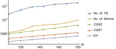
Figure 1: ‘TS’ refers to ‘Energetically Distinct Transition Sates’, ‘EH’ refers to the estimate of the number of minima given in ErberH95 , ‘CGS1’ is a recent Calef:2015 fit to the number of minima found in previous calculations, and ‘CGS2’ is an estimate Calef:2015 for the number of minima (we use the maximum out of those suggested in Calef:2015 .) The lines connecting data points are a guide to the eye.

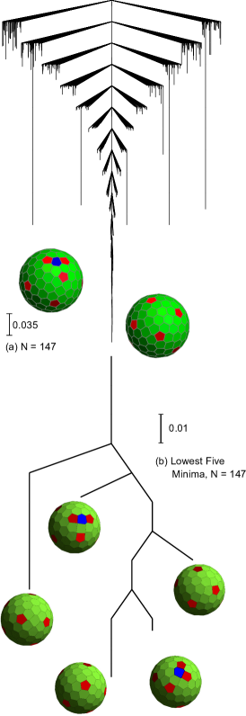
Figure 2: (a) The disconnectivity graph for $N=147$. In all cases considered here, the disconnectivity graphs show a typical structure-seeking ‘palm tree’ organisation. In panel (b) The insets show the structures of the lowest five minimum energy configurations. The pentagons, hexagons, and heptagons indicate that the charges in the centre of the polygons have 5, 6 and 7 neighbours respectively.

III Network Properties

For each $N$, we construct a network $G$ in which each node corresponds to a unique minimum energy structure, where permutation-inversion isomers are lumped together. Hence, there are $\mathcal{N}_{\mbox{min}}$ nodes. Two nodes are connected by an edge if a transition state exists between the corresponding minima. For each $N$ we have obtained $\mathcal{N}_{\mbox{ts}}$ energetically distinct transition states. Here we need only consider whether two minima are connected or not, and more than one distinct transition state between a pair of minima only counts as a single edge. We call $\mathcal{N}_{\mbox{edge}}$ the number of edges for the given network, with $\mathcal{N}_{\mbox{ts}}\geq\mathcal{N}_{\mbox{edge}}$. As in previous work for Lennard-Jones clusters Doye02 ; doye2005characterizing ; massen2005identifying , our networks are undirected and unweighted graphs, and hence agnostic about all other information, such as barrier heights or transition rates between the minima.

To further describe our findings, we first define two quantities. The characteristic path length ($L$) is the average of the shortest path between each pair of nodes in $G$. We apply an all-pairs shortest path algorithm cormen2009introduction to the graph $G$ to compute the distance between every two nodes. $L$ is the arithmetic mean of the distances between all pairs of nodes with a finite distance. The local clustering coefficient $C_{i}$ of the $i$th node is defined as the fraction of pairs of the neighbouring nodes that are connected over all pairs of the neighbours of the node. The global clustering coefficient $C$ is the average of $C_{i}$ for $i=1,\dots,\mathcal{N}_{\mbox{min}}$.

A graph is a small-world network if the characteristic path length is similar to, and the clustering coefficient is much higher than, the random graph with the same number of nodes and edges watts1998collective . Small-world properties have been observed in a number of networks of dynamic systems. Our results for the networks of minima of the Thomson Problem for various values of $N$ are reported in Table 1. The characteristic path length and the clustering coefficient of the corresponding random graph are denoted as $L_{0}$ and $C_{0}$, respectively. It is evident that $L$ is as small as $L_{0}$, while $C$ is much larger than $C_{0}$, and hence the small-world characteristics of the networks are established. The network diameter values, defined in terms of the longest shortest path length, are 5 ($N=132,135,138,141,144$), 6 ($N=147$) and 7 ($N=150$).

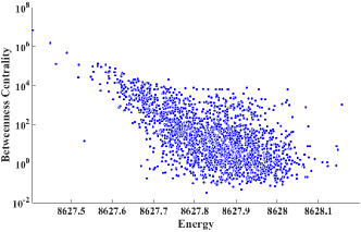
Figure 3: Betweenness centrality of the individual minima for $N=138$.

$N$	$\mathcal{N}_{\mbox{min}}$	$\mathcal{N}_{\mbox{ts}}$	$\mathcal{N}_{\mbox{edge}}$	$L$	$L_{0}$	$C$	$C_{0}$
132	1183	28284	8700	2.3003	2.8959	0.6032	0.0124
135	1585	51832	11285	2.2368	3.0391	0.6932	0.009
138	3226	88999	20150	2.1791	3.4865	0.6312	0.0039
141	4165	100085	38210	2.5684	3.1487	0.5871	0.0044
144	4534	136519	33113	2.3369	3.4445	0.7142	0.0032
147	6644	151299	39241	2.4314	3.8247	0.6375	0.0018
150	9774	178728	87203	2.7601	3.5163	0.4312	0.0018

Table 1: Analysis of networks for different values of $N$. $\mathcal{N}_{\mbox{min}}$, $\mathcal{N}_{\mbox{ts}}$ and $\mathcal{N}_{\mbox{edge}}$ are the number of minima (nodes), energetically distinct transition states, and edges, respectively. $L$ and $C$ are the characteristic path length and the clustering coefficient of each network, while $L_{0}$ and $C_{0}$ are the characteristic path length and the clustering coefficient of the corresponding random graph.

Another important network property is the betweenness centrality, which is defined for each node as the number of shortest paths from all nodes to all others that pass through the node under consideration. Betweenness centrality determines how central the node is. In Figure 3, we plot the betweenness centrality of all the nodes of our networks. Our results reveal that the global minimum of the Thomson Problem is always the most central in the network. The number of connections (the node degree) of minima as a function of energy is plotted in Figure 4. The figure clearly shows that low-lying minima are highly connected, making them hubs, unlike the higher energy minima.

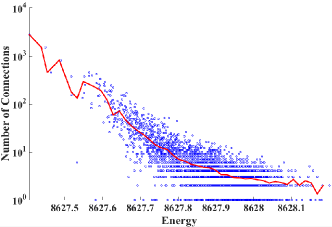
Figure 4: Potential energy minima vs the number of connection at the minimum is plotted, for $N=138$. The line is the binned average.

IV Discussion and Conclusion

In this paper we have characterised the potential energy landscape of the Thomson Problem for selected sizes up to $N=150$. We confirmed that both the number of minima and transition states grow exponentially with $N$, albeit with a small exponential factor due to the long range nature of the Coulomb interactions. This exponential increase makes the searches for the global minima of the Thomson Problem progressively more difficult. However, by analysing the disconnectivity graphs, we find that for the sizes investigated here, the landscapes exhibit clear structure-seeking organisation. The global minima for systems characterised by such funnelled potential energy landscapes can usually be located easily, even when the total number of minima is large. The asymmetry of the energy barriers makes it easy to escape from high to low energy minima, while the reverse transitions are significantly slower.

We have analysed the networks consisting of local minima and the connections between them defined by transition states, and find that they exhibit small world properties watts1998collective . Our results provide further evidence to support the conjecture that the small-world phenomenon might be another generic feature of landscapes with the structure-seeking ‘palm tree’ organisation CarrW08 . Moreover, we found that the low-lying minima are generally significantly more connected than those at higher energy, suggesting scale-free properties. Further statistical tests clauset2009power are required to confirm this behaviour. We note that similar kinetic hubs have been identified for biomolecules in previous work CavalliHPC03 ; GfellerdDCR07 ; CarrW08 . It is important to note that these networks are static. Hence, the scale-free phenomenon, if confirmed, requires explanation beyond the usual preferential attachment schemes BarabasiA99 .

Our results are relevant for addressing Smale’s 7th problem. For the sizes considered here, the global minimum is, on average, only a few transition states [$O(\log\mathcal{N}_{\mbox{min}})$] away from any random starting point. $\mathcal{N}_{\mbox{min}}$ grows exponentially with $N$, and the increase in the average number of connections is linear. Since the diameter of the networks is typically 5 or 6 (and at most 7), the global minimum is never further than a few steps away, even from the highest-lying minimum. Moreover, the betweenness centrality is largest, by orders of magnitude, for the global minimum, so the majority of shortest paths between all pairs of minima pass through the global minimum, i.e. the global minimum is the central node of these networks. Hence finding the global minimum and exploiting the funnelled/small-world structure of the landscape, is relatively straightforward from a numerical optimisation point of view. Interestingly, though our results suggest that finding the global minimum of the Thomson Problem may be relatively easy, finding an answer to the Smale problem is NP-hard beltran2013harmonic . Constructing and analysing network of minima for the logarithmic version of the potential smale1998mathematical-2 may provide more concrete details on the mathematics behind Smale’s 7th problem.

The present results agree with the observation Doye02 that funnelled energy landscapes display small world characteristics. In the future we will explore whether these two features are generally correlated, or if a counterexample can be found. Another avenue for future work is to extend our analysis to larger particle numbers. Our previous work on the Thomson Problem wales2006structure found that global minima for for $N>400$ start to display alternative defect motifs. We expect the potential energy landscape to display multiple funnels in this regime, and it will be interesting to see whether the small world phenomenon found here will be preserved.

In the future, we will further analyse the network properties of this model by including weights and directions for the edges, depending on the barrier heights and kinetic transition rates. We also plan to develop more specific algorithms to locate local and global minima by exploiting small-world properties mehta2014communication ; mehta2015exploring ; chen2015index . Analysing the appropriately weighted and directed networks of free energy minima rao2004protein and transition states may provide additional insight into the Thomson Problem. Furthermore, invesetigating network properties of higher index saddles may also provide insights to develop novel optimization algorithms hughes2014inversion .

V Acknowledgement

DM was supported by a Australian Research Council DECRA fellowship no. DE140100867. DZC was supported in part by the NSF under Grant CCF-1217906. We thank Carlos Beltrán and Edward Saff for their helpful remarks the authors of Calef:2015 for clarifying their results.

References

- (1) J. J. Thomson, The London, Edinburgh, and Dublin Philosophical Magazine and Journal of Science 7, 237 (1904).
- (2) D. L. Caspar and A. Klug, Physical principles in the construction of regular viruses, in Cold Spring Harbor symposia on quantitative biology, volume 27, pages 1–24, Cold Spring Harbor Laboratory Press, 1962.
- (3) C. J. Marzec and L. A. Day, Biophysical journal 65, 2559 (1993).
- (4) R. F. Bruinsma, W. M. Gelbart, D. Reguera, J. Rudnick, and R. Zandi, Physical review letters 90, 248101 (2003).
- (5) R. Zandi, D. Reguera, R. F. Bruinsma, W. M. Gelbart, and J. Rudnick, PNAS 101, 15556 (2004).
- (6) H. W. Kroto et al., Nature 318, 162 (1985).
- (7) E. J. Davis, Aerosol Science and Technology 26, 212 (1997).
- (8) A. R. Bausch et al., Science 299, 1716 (2003).
- (9) P. Lipowsky, M. J. Bowick, J. H. Meinke, D. R. Nelson, and A. R. Bausch, Nat. Mater. 4, 407 (2005).
- (10) T. Einert, P. Lipowsky, J. Schilling, M. J. Bowick, and A. R. Bausch, Langmuir 21, 12076 (2005).
- (11) H. Kusumaatmaja and D. J. Wales, Phys. Rev. Lett. 110, 165502 (2013).
- (12) G. Meng, J. Paulose, D. R. Nelson, and V. N. Manoharan, Science 343, 634 (2014).
- (13) W. T. M. Irvine, V. Vitelli, and P. M. Chaikin, Nature 468, 947 (2010).
- (14) W. T. M. Irvine, M. J. Bowick, and P. M. Chaikin, Nat. Mater. 11, 948 (2012).
- (15) E. Bendito, M. J. Bowick, A. Medina, and Z. Yao, Phys. Rev. E 88, 012405 (2013).
- (16) S. Smale, The Mathematical Intelligencer 20, 7 (1998).
- (17) S. Smale, Lecture given on the occasion of Arnold’s 60th birthday at the Fields Institute, Toronto. (1997).
- (18) Smale’s 7th problem rather considers a general form of the potential, , with the spherical constraints. The special values and correspond to a logarithmic potential and the Thomson Problem, respectively. In Ref. smale1998mathematical-2 is considered as the ‘main’ problem (and the Thomson Problem listed as a special case of the general problem) and more mathematicians are focused on this version of the problem. is a popular model in chemistry and physics. In the asymptotic limit, both versions of the problems are similar in the following sense: a solution to Thomson Problem is known to have an asymptotically optimal logarithmic potential. This statement is proven both ways in Refs. leopardi2013discrepancy ; beltran2015facility . In any case, both versions of the problem share the same importance and qualitative features.
- (19) L. Blum, F. Cucker, M. Shub, and S. Smale, Complexity and real computation, Springer Science & Business Media, 2012.
- (20) M. Shub and S. Smale, J. Complexity 9, 4 (1993).
- (21) D. Armentano, C. Beltrán, and M. Shub, Transactions of the American Mathematical Society 363, 2955 (2011).
- (22) L. T. Wille, Nature 324, 46 (1986).
- (23) T. Erber and G. M. Hockney, J. Phys. A 24, L1369 (1991).
- (24) E. L. Altschuler, T. J. Williams, E. R. Ratner, F. Dowla, and F. Wooten, Phys. Rev. Lett. 72, 2671 (1994).
- (25) T. Erber and G. M. Hockney, Phys. Rev. Lett. 74, 1482 (1995).
- (26) E. L. Altschuler et al., Phys. Rev. Lett. 78, 2681 (1997).
- (27) T. Erber and G. M. Hockney, Adv. Chem. Phys. 98, 495 (1997).
- (28) J. R. Morris, D. M. Deaven, and K. M. Ho, Phys. Rev. B 53, R1740 (1996).
- (29) E. L. Altschuler and A. Pérez-Garrido, Phys. Rev. E 71, 047703 (2005).
- (30) E. L. Altschuler and A. Perez-Garrido, Phys. Rev. E 73, 036108 (2006).
- (31) D. J. Wales and S. Ulker, Phys. Rev. B 74, 212101 (2006).
- (32) D. J. Wales, H. McKay, and E. L. Altschuler, Phys. Rev. B 79, 224115 (2009).
- (33) J. S. Brauchart, D. P. Hardin, and E. B. Saff, Bulletin of the London Mathematical Society 41, 621 (2009).
- (34) J. Brauchart, D. Hardin, and E. Saff, Contemp. Math 578, 31 (2012).
- (35) M. Bowick, C. Cecka, and A. Middleton, Thomson problem @ s.u., http://physics.syr.edu/condensedmatter/thomson/thomson.htm.
- (36) N. N. Andreev, East J. Approx 2, 459 (1996).
- (37) R. E. Schwartz, arXiv preprint arXiv:1001.3702 (2010).
- (38) E. B. Saff and A. B. Kuijlaars, The mathematical intelligencer 19, 5 (1997).
- (39) A. Kuijlaars and E. Saff, Transactions of the American Mathematical Society 350, 523 (1998).
- (40) A. Pérez-Garrido and M. A. Moore, Phys. Rev. B 60, 15628 (1999).
- (41) A. M. Livshits and Y. E. Lozovik, Chem. Phys. Lett. 314, 577 (1999).
- (42) M. J. Bowick, D. R. Nelson, and A. Travesset, Phys. Rev. B 62, 8738 (2000).
- (43) M. Bowick, A. Cacciuto, D. R. Nelson, and A. Travesset, Phys. Rev. Lett. 89, 185502 (2002).
- (44) M. J. Bowick, A. Cacciuto, D. R. Nelson, and A. Travesset, Phys. Rev. B 73, 024115 (2006).
- (45) L. Giomi and M. J. Bowick, Phys. Rev. E 78, 010601 (2008).
- (46) T. LaFave Jr, Journal of Electrostatics 72, 39 (2014).
- (47) O. M. Becker and M. Karplus, J. Chem. Phys. 106, 1495 (1997).
- (48) D. J. Wales, M. A. Miller, and T. R. Walsh, Nature 394, 758 (1998).
- (49) J. N. Murrell and K. J. Laidler, Trans. Faraday. Soc. 64, 371 (1968).
- (50) F. Noé and S. Fischer, Curr. Op. Struct. Biol. 18, 154 (2008).
- (51) D. Prada-Gracia, J. Gómez-Gardenes, P. Echenique, and F. Fernando, PLoS Comput. Biol. 5, e1000415 (2009).
- (52) D. J. Wales, Curr. Op. Struct. Biol. 20, 3 (2010).
- (53) D. J. Wales, Gmin: A program for basin-hopping global optimisation, basin-sampling, and parallel tempering, http://www-wales.ch.cam.ac.uk/software.html.
- (54) D. J. Wales, Optim: A program for geometry optimisation and pathway calculations, http://www-wales.ch.cam.ac.uk/software.html.
- (55) Z. Li and H. A. Scheraga, Proc. Natl. Acad. Sci. USA 84, 6611 (1987).
- (56) D. J. Wales and J. P. K. Doye, J. Phys. Chem. A 101, 5111 (1997).
- (57) D. J. Wales and H. A. Scheraga, Science 285, 1368 (1999).
- (58) D. J. Wales, Energy Landscapes, Cambridge University Press, Cambridge, 2003.
- (59) J. Nocedal, Mathematics of Computation 35, 773 (1980).
- (60) D. Liu and J. Nocedal, Math. Prog. 45, 503 (1989).
- (61) D. Asenjo, J. D. Stevenson, D. J. Wales, and D. Frenkel, J. Phys. Chem. B 117, 12717 (2013).
- (62) S. A. Trygubenko and D. J. Wales, J. Chem. Phys. 120, 2082 (2004).
- (63) G. Henkelman, B. P. Uberuaga, and H. Jónsson, J. Chem. Phys. 113, 9901 (2000).
- (64) L. J. Munro and D. J. Wales, Phys. Rev. B 59, 3969 (1999).
- (65) Y. Kumeda, L. J. Munro, and D. J. Wales, Chem. Phys. Lett. 341, 185 (2001).
- (66) We compare our results with the estimate on the number of minima, , as given in ErberH95 , the number of minima from a fit to the number of minima found, and estimated number of minima (with choosing the ’’ sign for both ’’ in our comparison), as given in Calef:2015 .
- (67) M. Calef, W. Griffiths, and A. Schulz, J. of Stat. Phys. , 1 (2015).
- (68) F. H. Stillinger and T. A. Weber, Science 225, 983 (1984).
- (69) D. J. Wales and J. P. K. Doye, J. Chem. Phys. 119, 12409 (2003).
- (70) J. P. K. Doye, D. J. Wales, and R. S. Berry, J. Chem. Phys. 103, 4234 (1995).
- (71) J. P. K. Doye and D. J. Wales, Science 271, 484 (1996).
- (72) J. P. K. Doye and D. J. Wales, J. Chem. Soc., Faraday Trans. 93, 4233 (1997).
- (73) J. P. K. Doye, Phys. Rev. Lett. 88, 238701 (2002).
- (74) J. P. Doye and C. P. Massen, The Journal of chemical physics 122, 084105 (2005).
- (75) C. P. Massen and J. P. Doye, Physical Review E 71, 046101 (2005).
- (76) T. H. Cormen, C. E. Leiserson, R. L. Rivest, and C. Stein, Introduction to Algorithms, MIT press, 3rd edition, 2009.
- (77) D. J. Watts and S. H. Strogatz, nature 393, 440 (1998).
- (78) J. M. Carr and D. J. Wales, J. Phys. Chem. B 112, 8760 (2008).
- (79) A. Clauset, C. R. Shalizi, and M. E. Newman, SIAM review 51, 661 (2009).
- (80) A. Cavalli, U. Haberthür, E. Paci, and A. Caflisch, Prot. Sci. 12, 1801 (2003).
- (81) D. Gfeller, D. M. de Lachapelle, P. De Los Rios, G. Caldarelli, and F. Rao, Phys. Rev. E 76, 026113 (2007).
- (82) A. L. Barabási and R. Albert, Science 286, 509 (1999).
- (83) C. Beltrán, Constructive Approximation 37, 135 (2013).
- (84) D. J. Wales and S. Ulker, Physical Review B 74, 212101 (2006).
- (85) D. Mehta, T. Chen, J. D. Hauenstein, and D. J. Wales, The Journal of chemical physics 141, 121104 (2014).
- (86) D. Mehta, T. Chen, J. W. Morgan, and D. J. Wales, The Journal of chemical physics 142, 194113 (2015).
- (87) T. Chen and D. Mehta, arXiv preprint arXiv:1504.06622 (2015).
- (88) F. Rao and A. Caflisch, Journal of molecular biology 342, 299 (2004).
- (89) C. Hughes, D. Mehta, and D. J. Wales, The Journal of chemical physics 140, 194104 (2014).
- (90) P. Leopardi, Advances in Computational Mathematics , 1 (2013).
- (91) C. Beltrán, Foundations of Computational Mathematics 15, 125 (2015).