Persistent current in a 2D Josephson junction array wrapped around a cylinder

Abstract

We study persistent currents in a Josephson junction array wrapped around a cylinder. The $T=0$ quantum statistical mechanics of the array is equivalent to the statistical mechanics of a classical $xy$ spin system in 2+1 dimensions at the effective temperature $T^{*}=\sqrt{2JU}$, with $J$ being the Josephson energy of the junction and $U$ being the charging energy of the superconducting island. It is investigated analytically and numerically on lattices containing over one million sites. For weak disorder and $T^{*}\ll J$ the dependence of the persistent current on disorder and $T^{*}$ computed numerically agrees quantitatively with the analytical result derived within the spin-wave approximation. The high-$T^{*}$ and/or strong-disorder behavior is dominated by instantons corresponding to the vortex loops in 2+1 dimensions. The current becomes destroyed completely at the quantum phase transition into the Cooper-pair insulating phase.

I Introduction

Persistent currents in closed chains of Josephson junctions (JJ) have been studied for more than two decades (see, e.g. Refs. Choi-1993, ; Matveev, ; Pop, ; Rastelli, ; garchu-PRB16, and references therein). Being conceptually similar to small superconducting rings they provide a testing ground for models of quantum phase slips Zaikin ; Golubev ; Oreg ; Semenov-PRB13 and superconductor-insulator transition (SIT) Bradley ; Korshunov ; Chow . This research has significantly intensified in recent years due to advances in manufacturing of nanostructures Mooij-2015 and the renewed interest to quantum phase transitions Girvin ; Sachdev inspired in part by the prospects of applications of quantum circuitry Ioffe ; Gladchenko ; Manucharyan .

There exist even a greater volume of work on SIT in disordered ultrathin films (see, e.g. Ref. Goldman, and references therein). Similar to superconducting rings, various mechanisms of SIT have been modeled by two-dimensional JJ arrays Fazio-Schon ; Imry ; Vinokur ; Altshuler ; EC . To have a persistent current in a $2D$ JJ array the latter should be closed into a cylindrical surface that encloses the magnetic flux, see Fig. 1. In this Letter we argue that studies of persistent currents in such a system provides another avenue for testing the theory of quantum phase transitions. It may also be relevant to properties of an ultrathin superconducting film deposited on a cylinder and properties of a superconducting topological insulator Bernevig .

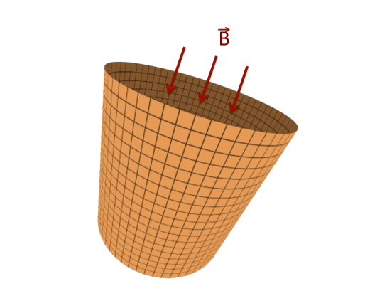
Figure 1: Color online: A $2D$ JJ array wrapped around a cylinder that encloses the magnetic flux.

A system that bears some relevance to the JJ array wrapped around a cylinder is a JJ ladder made of capacitively coupled one-dimensional JJ rings, e.g., JJ necklaces stuck together. It was studied theoretically by the numerical density-matrix renormalization group with an emphasis on the role of excitons Lee-PRB03 . In this Letter we are taking a different approach. When the dynamics of the $2D$ JJ array is dominated by capacitances of superconducting islands its $T=0$ quantum statistical mechanics is equivalent Bradley ; Choi-1993 ; Wallin-94 ; Girvin ; Kim-08 to the statistical mechanics of the classical $xy$ spin system in $2+1$ dimensions at the effective temperature $T^{*}=\sqrt{2JU}$, with $J$ being the Josephson energy of the junction and $U$ being the charging energy of the superconducting island. The advantage of such a mapping is its suitability for large-scale Monte Carlo (MC) studies.

To make this problem relevant to experimental systems it must also include disorder. Positional disorder in a planar JJ array is known to give rise to random phases when the array is placed in the transverse magnetic field Granato . The resulting “gauge” or “Bose” glass has been intensively studied by analytical Rubinstein ; KorNat ; Li ; Gupta and numerical Tang ; Kim-06 ; Kim-08 methods. Phase disorder has been found to have a significant effect on the SIT. The model with the transverse magnetic field would not apply to the JJ array wrapped around a cylinder. However, static random phases in Josephson junctions can also be generated by other mechanisms, e.g., by the broken time-reversal symmetry in the presence of the magnetic moments Buzdin-PRL08 ; Buzdin-PRL09 .

At first we neglect disorder. Let $\theta_{ij}$ be the phase of the superconducting order parameter $\Psi=|\Psi|\exp(i\theta)$ at the $ij$-th superconducting island, with $i=1,2,...,N$ denoting the islands in the $j$-th ring ($j=1,2,...,N$) of the $2D$ JJ array shown in Fig. 1. The Josephson energy of the array is Tinkham

$$E_{J}=J\sum_{ij}\left[1-\cos\left(\theta_{i,j+1}-\theta_{ij}\right)\right]+$$

$$J\sum_{ij}\left[1-\cos\left(\theta_{i+1,j}-\theta_{ij}+\frac{2\pi}{\Phi_{0}}\int_{i}^{i+1}{\bf A}\cdot d{\bf l}_{j}\right)\right],$$

(1)

where the vector potential ${\bf A}$ is due to the magnetic flux $\Phi$ enclosed by the cylinder.

Summation along each $j$-th ring gives

$$\sum_{i}\left(\theta_{i+1,j}-\theta_{ij}\right)=2\pi m_{j},\quad\frac{2\pi}{\Phi_{0}}\sum_{i}\int_{i}^{i+1}{\bf A}\cdot d{\bf l}_{j}=2\pi\phi,$$ (2)

where $\phi\equiv\Phi/\Phi_{0}$, $\Phi_{0}=h/(2e)$ is the flux quantum, and $m_{j}$ is an integer. This allows one to write

$$E_{J}=J\sum_{ij}\left[1-\cos\left(\tilde{\theta}_{i,j+1}-\tilde{\theta}_{ij}\right)\right]+$$

$$J\sum_{ij}\left[1-\cos\left(\tilde{\theta}_{i+1,j}-\tilde{\theta}_{ij}+\frac{2\pi\left(\phi+m_{j}\right)}{N}\right)\right],$$ (3)

where the reduced phases $\tilde{\theta}$ are defined in such a way that the change of $\tilde{\theta}_{i}$ around the $j$-th ring is zero. The total accumulation of the original phase $\theta_{ij}$ in a closed path around the cylinder is accounted for by the quantum number $m_{j}$. The persistent current in the cylinder is given by

$$I=\frac{d\left\langle E_{J}\right\rangle}{d\Phi}=\frac{1}{\Phi_{0}}\frac{d\left\langle E_{J}\right\rangle}{d\phi},$$ (4)

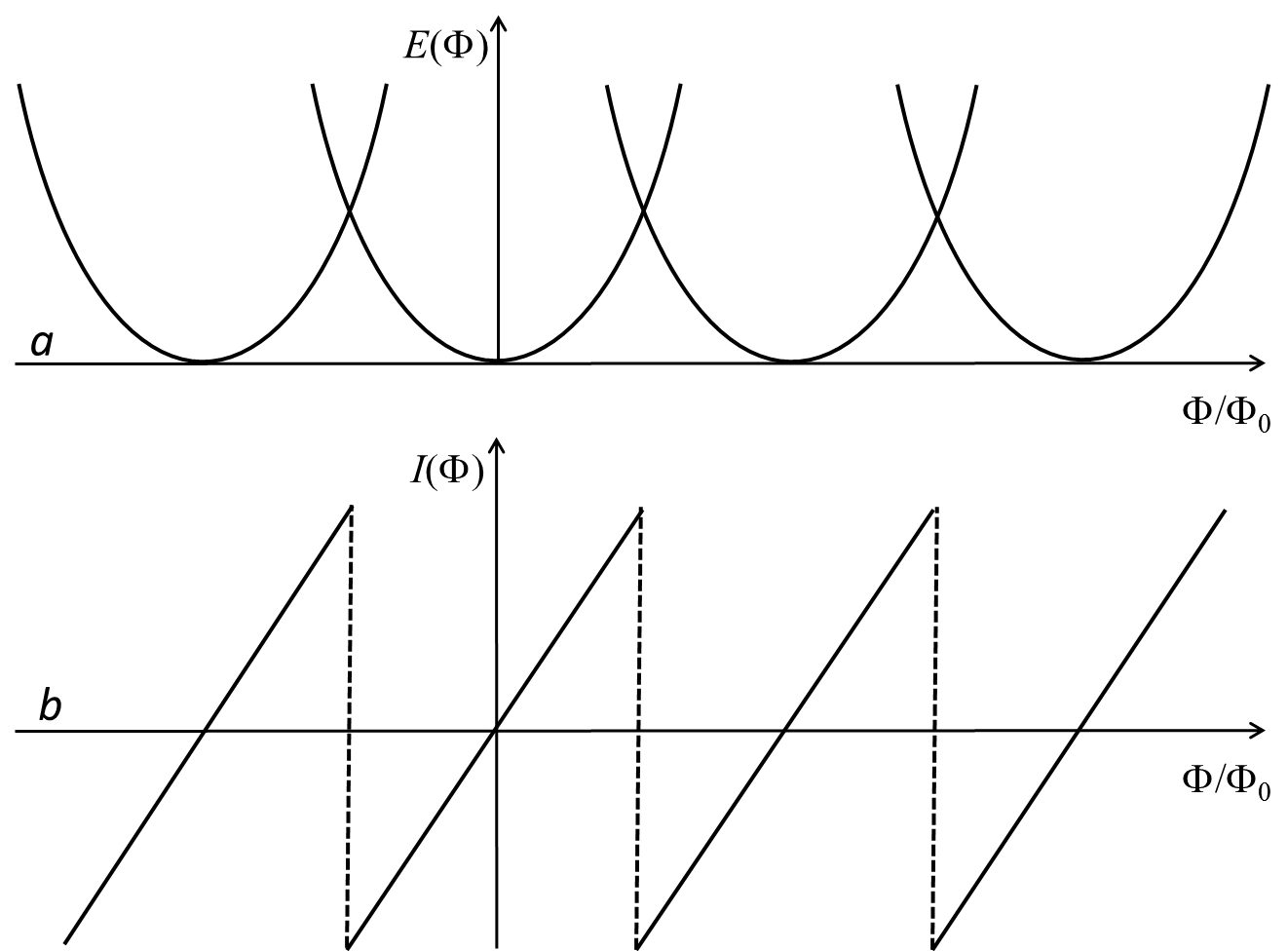
Figure 2: ($a$) $m$-branches of the ground-state energy $E_{J}^{(0)}$. ($b$) $m$-branches of the persistent current.

The energy minimum corresponds to all $\tilde{\theta}_{ij}$ and all $m_{j}$ being the same ($m_{j}=m$), leading to the ground state

$$E_{J}^{(0)}=JN^{2}\left[1-\cos\left(\frac{2\pi\left(\phi+m\right)}{N}\right)\right]\cong 2\pi^{2}J(\phi+m)^{2},$$ (5)

the last expression being the large-$N$ case. Branches of $E_{J}^{(0)}(\Phi)$ and $I^{(0)}(\Phi)={dE_{J}^{(0)}}/{d\Phi}$ for different values of $m$ are shown in Fig. 2$a$ and Fig. 2$b$ respectively. When $\phi=n+1/2$, with $n$ being an integer, that is for $\Phi=(n+1/2)\Phi_{0}$, the ground state is degenerate, $E_{J}(n,m)=E_{J}(n,m^{\prime}=-2n-m-1)$. For, e.g., half a fluxon, $\Phi=\Phi_{0}/2$, the current has the same absolute value but flows in opposite directions for $m=0$ and $m=-1$.

The dynamics of the JJ array is due to the electrical charging of the superconducting islands by the excess (or lack) of Cooper pairs $n_{ij}$ at the $ij$-th site. It is determined by the finite capacitances of the islands to the ground and the capacitances of the junctions. Different limits, with both capacitances present, can be achieved in experiment and have been studied in literature, see, e.g., Ref. Rastelli, and references therein. In this paper we are considering the limit in which the capacitances of the islands, $C$, greatly exceed the capacitances of the junctions. In this case the charging energy is given by

$$E_{C}=\sum_{ij}Un_{ij}^{2}=\frac{\hbar^{2}}{4U}\sum_{ij}\left(\frac{d\theta_{ij}}{dt}\right)^{2}$$ (6)

where $U=(2e)^{2}/(2C)$. The second of Eq. (6), which plays the role of the kinetic energy, is obtained by noticing that $n_{ij}$ and $\theta_{ij}$ are canonically conjugated variables, $n_{ij}=-i{d}/{d\theta_{ij}}$, so that $i\hbar{d\theta_{ij}}/{dt}=[\theta_{i},E_{C}]=2iUn_{i}$. Finite $U$ permits quantum tunneling between the current states that correspond to $E_{J}(n,m)$ and $E_{J}(n,m^{\prime})$.

The Lagrangian of the model is ${\cal{L}}=E_{C}-E_{J}$. Its quantum mechanics is formulated in terms of the path integral

$${\cal{I}}=\prod_{i}\int D\{\theta_{i}(\tau)\}e^{-S_{E}/\hbar}$$ (7)

where $\tau=it$ and $S_{E}=\int d\tau{\cal L}$ is the Euclidean action with

$${\cal L} = \frac{\hbar^{2}}{4U}\sum_{ij}\left(\frac{d\theta_{ij}}{d\tau}\right)^{2}+J\sum_{ij}\left[1-\cos\left(\theta_{i,j+1}-\theta_{ij}\right)\right]$$ (8)

$$+ J\sum_{ij}\left[1-\cos\left(\theta_{i+1,j}-\theta_{ij}+\frac{2\pi\phi}{N}\right)\right].$$

Statistical mechanics of this quantum model at $T=0$ is equivalent Bradley ; Choi-1993 ; Wallin-94 ; Girvin ; Kim-08 to the statistical mechanics of the classical model in 2+1 dimensions at a non-zero temperature $T^{*}=\sqrt{2JU}$, described by the partition function

$$Z=\prod_{i}\int D\{\theta_{i}(\tau)\}e^{-\mathcal{H}_{2+1}/T^{*}}$$ (9)

with $\mathcal{H}_{1+1}=-\frac{1}{2}\sum_{\mathbf{rr}^{\prime}}J_{\mathbf{rr}^{\prime}}\cos\left(\theta_{\mathbf{r}^{\prime}}-\theta_{\mathbf{r}}+\phi_{\mathbf{rr}^{\prime}}\right)$, where $\mathbf{r}$ is a discrete three-dimensional vector $\mathbf{r}=(i,j,l)$ representing the space-time lattice, while $J_{\mathbf{rr}^{\prime}}=J$ for the nearest neighbors and zero otherwise. In the numerical work we use the $N\times N\times N$ lattice with the $l$ direction corresponding to the imaginary time and periodic boundary consitions. Non-zero phase shifts are given by $\phi_{i,j,l;i\pm 1,j,l}=\pm 2\pi\phi/N$. Notice that, in principle, the periodic boundary condition imposed on the imaginary time introduces a finite physical temperature into the original quantum problem, $T\sim T^{*}/N$. At large $N$ the effect of that temperature on the persistent current can be ignored.

The statistical model presented above can be reformulated in terms of the three-component classical spin vectors of the $3D$ $xy$ model at temperature $T^{*}=\sqrt{2JU}$ that describes the strength of quantum fluctuations. That model has a ferromagnetic-paramagnetic phase transition at $T^{*}=T_{c}$ that in the original model corresponds to the quantum phase transition into the Cooper-pair insulator state in which the islands connected by Josephson junctions maintain their superconductivity but no Josephson current can circulate around the cylinder. The natural way to test this prediction is to study the dependence of the persistent current on $U$.

Phase slips corresponding to quantum tunneling between different $m$ require formation of vortex loops in 2+1 dimensions. At small $U$ satisfying $T^{*}=\sqrt{2JU}\ll T_{c}\sim J$ such loops nucleate with exponentially small probability. Consequently, at a small $T^{*}$, if one induces a persistent current by placing the cylinder with the JJ array in the magnetic field, the phase slips may not occur on the time scale of the experiment. In this case all $m_{j}$ in Eq. 3 are the same, $m_{j}=m$, and the persistent current computed with the help of Eq. (4) and the symmetry becomes

$$I=\frac{2\pi NJ}{\Phi_{0}}\sin\left[\frac{2\pi\left(\phi+m\right)}{N}\right]\langle\cos(\tilde{\theta}_{i,j,l}-\tilde{\theta}_{i+1,j,l})\rangle.$$ (10)

We now recall that the statistical mechanics of our model is that of the $3D$ $xy$ model at $T=T^{*}$, for which the low-temperature (spin-wave) result for the cubic lattice is $\left\langle\cos\left(\theta_{\mathbf{r}}-\theta_{\mathbf{r}+\boldsymbol{\delta}}\right)\right\rangle=1-T^{*}/(6J)$, with $\boldsymbol{\delta}$ being the nearest neighbor in any direction. This gives for large $N$

$$I\cong\frac{\left(2\pi\right)^{2}J}{\Phi_{0}}(\phi+m)\left(1-\frac{T^{*}}{6J}\right).$$ (11)

We shall now consider the effect of quenched disorder by adding a static random phase $\phi_{ij}$ to the phase difference, $\theta_{i,j+1}-\theta_{ij}$, between neighboring superconducting islands $i$ and $j$ in Eq. (1). In the models of planar JJ arrays such random phase can be generated by the positional disorder in the $2D$ lattice of Josephson junctions in the presence of the transverse magnetic field Granato ; KorNat ; Li ; Gupta ; Tang ; Kim-06 ; Kim-08 . In our case of a JJ array wrapped around a cylinder, random phases can be generated due to, e.g., anomalous Josephson effect in the presence of magnetic moments Buzdin-PRL08 ; Buzdin-PRL09 .

As was shown in Ref. Rubinstein, the continuous counterpart of the model with quenched randomness corresponds to the interaction of the continuous phase order parameter $\theta({\bf r})$ with a static random field ${\bf q}({\bf r})=\phi_{ij}\hat{r}_{ij}/a$ ($a$ being the lattice spacing), described by

$$E_{J}=\frac{1}{2}J\int d^{2}r[{\bm{\nabla}}\theta({\bf r})-{\bf q}({\bf r})]^{2}.$$ (12)

The Imry-Ma argument I-M favors the destruction of the long-range order in less than four dimensions by a weak static random field interacting with the order parameter directly, since at $d<4$ such interaction, regardless of strength, dominates the energy at large distances. Crucial to that argument, however, is the formation of topological defects which makes the order more robust PGC-PRL2014 . In our case, random field in Eq. (12) interacts with the gradient of the order parameter, which further diminishes its effect at large distances. One should expect, therefore, that the initially ordered state will not be destroyed by weak quenched randomness at low $T^{*}$.

The persisent current in Eq. (10) should now be calculated with account of averaging over phase fluctuations generated by the random field. Introducing random phases $\phi_{ij}$ into Eq. (3), similarly to the above in the limit of large $N$ we obtain

$$I=\frac{(2\pi)^{2}J\left(\phi+m\right)}{\Phi_{0}}\left\langle\cos\left[\tilde{\theta}_{i+1,j,l}-\tilde{\theta}_{i,j,l}+\phi_{ij}\right]\right\rangle.$$ (13)

In the case $|\phi_{ij}|\ll 1$ and $|\tilde{\theta}_{i+1,j,l}-\tilde{\theta}_{i,j,l}|\ll 1$ the continuous model of Eq. (12) yields

$$I=\frac{(2\pi)^{2}J\left(\phi+m\right)}{\Phi_{0}}\left\{1-\frac{1}{2}a^{2}\left\langle[{\bm{\nabla}}\theta({\bf r})-{\bf q}({\bf r})]^{2}\right\rangle\right\}.$$ (14)

The effects of low temperature and weak static randomness must be additive. It suffices, therefore, to compute the contribution of quenched randomness at $T^{*}=0$ just minimizing the energy, Eq. (12). The extrema of the latter satisfy the equation

$${\bm{\nabla}}^{2}\theta({\bf r})={\bm{\nabla}}\cdot{\bf q}({\bf r})$$ (15)

having the solution

$$\theta({\bf r})=\int d^{2}r^{\prime}G({\bf r}-{\bf r}^{\prime}){\bm{\nabla}}\cdot{\bf q}({\bf r}^{\prime})=\int d^{2}r^{\prime}{\bf q}({\bf r}^{\prime})\cdot{\bm{\nabla}}G({\bf r}-{\bf r}^{\prime}),$$ (16)

where $G({\bf r})=(2\pi)^{-1}\ln(r/a)$ is the Green function of the $2D$ Laplace equation, ${\bm{\nabla}}^{2}G({\bf r})=\delta({\bf r})$. With the help of this equation one obtains

$${\nabla}_{\alpha}\theta({\bf r})-q_{\alpha}({\bf r})=$$

$$\int d^{2}r^{\prime}q_{\beta}({\bf r}^{\prime})\left[{\nabla}_{\alpha}\nabla_{\beta}G({\bf r}-{\bf r}^{\prime})-\delta_{\alpha\beta}\delta({\bf r}-{\bf r}^{\prime})\right],$$ (17)

so that

$$[{\bm{\nabla}}\theta({\bf r})-{\bf q}({\bf r})]^{2}=\int d^{2}r^{\prime}\int d^{2}r^{\prime\prime}q_{\beta}({\bf r}^{\prime})q_{\gamma}({\bf r}^{\prime\prime})$$

$$\times\left[{\nabla}_{\alpha}\nabla_{\beta}G({\bf r}-{\bf r}^{\prime})-\delta_{\alpha\beta}\delta({\bf r}-{\bf r}^{\prime})\right]$$

$$\times\left[{\nabla}_{\alpha}\nabla_{\gamma}G({\bf r}-{\bf r}^{\prime\prime})-\delta_{\alpha\gamma}\delta({\bf r}-{\bf r}^{\prime\prime})\right].$$ (18)

We shall assume that

$$\langle q_{\beta}({\bf r}^{\prime})q_{\gamma}({\bf r}^{\prime\prime})\rangle=\frac{1}{2}a^{2}q_{R}^{2}\delta_{\beta\gamma}\delta({\bf r}^{\prime}-{\bf r}^{\prime\prime}).$$ (19)

Then

$$\left\langle[{\bm{\nabla}}\theta({\bf r})-{\bf q}({\bf r})]^{2}\right\rangle=$$

$$\frac{1}{2}a^{2}q_{R}^{2}\int d^{2}r\left[{\nabla}_{\alpha}\nabla_{\beta}G({\bf r})-\delta_{\alpha\beta}\delta({\bf r})\right]^{2}$$

$$=\frac{1}{2}a^{2}q_{R}^{2}\int\frac{d^{2}k}{(2\pi)^{2}}\left[k_{\alpha}k_{\beta}G({\bf k})+\delta_{\alpha\beta}\delta({\bf k})\right]^{2}$$

$$=\frac{1}{2}a^{2}q_{R}^{2}\int\frac{d^{2}k}{(2\pi)^{2}}\left[\delta_{\alpha\beta}-\frac{k_{\alpha}k_{\beta}}{k^{2}}\right]^{2}$$

$$=\frac{1}{2}a^{2}q_{R}^{2}\int\frac{d^{2}k}{(2\pi)^{2}}=\frac{1}{2}q_{R}^{2},$$ (20)

where we have used Fourier transforms: $G({\bf k})=-1/k^{2}$ and $\delta({\bf k})=1$. Thus

$$I=\frac{(2\pi)^{2}J\left(\phi+m\right)}{\Phi_{0}}\left(1-\frac{1}{4}a^{2}q_{R}^{2}\right).$$ (21)

The last step is to establish the relation between $q_{R}$ and $\phi_{R}$ used in the numerical experiment. If $\phi_{ij}$ are chosen randomly between $-\phi_{R}$ and $\phi_{R}$, one has

$$a^{2}q_{R}^{2}=\frac{1}{2\phi_{R}}\int_{-\phi_{R}}^{+\phi_{R}}d\phi\,\phi^{2}=\frac{\phi_{R}^{2}}{3}.$$ (22)

Inserting this into the above formula and combining it with Eq. (11), one finally obtains the persistent current at low $T^{*}$ in the presence of weak randomness

$$I=\frac{(2\pi)^{2}J\left(\phi+m\right)}{\Phi_{0}}\left(1-\frac{T^{*}}{6J}-\frac{\phi_{R}^{2}}{12}\right).$$ (23)

As we shall see, this formula agrees well with numerical results.

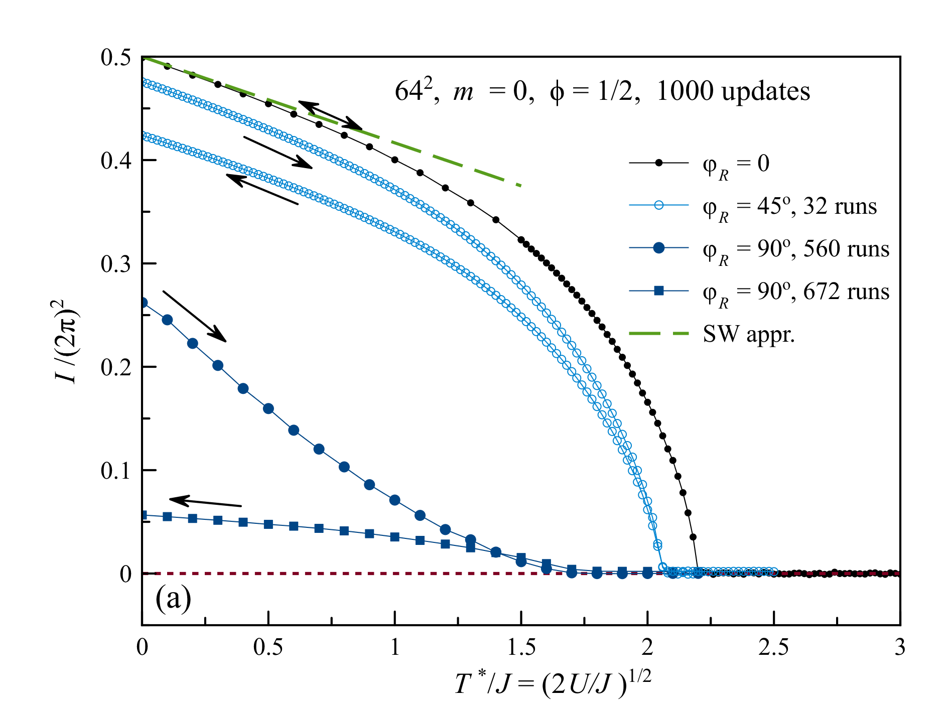
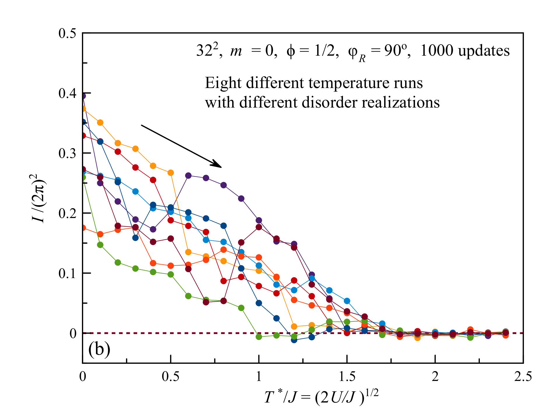
Figure 3: Color online: Effective-temperature dependence of the persistent current. (a) Averaged over disorder realizations (runs). (b) Individual runs showing strong fluctuations for strong disorder.

Higher $T^{*}$ and $\phi_{R}$ tend to create topological defects. Destruction of the persistent current by the latter and spin waves can be investigated numerically using the equivalent magnetic model of two-component vectors $\mathbf{s}$ of fixed length instead of the grain phase $\theta$.

The case $T^{*}=0$ is classical, so that one can minimize the energy of the $2D$ system of Josephson grains by the method of Ref. garchu-PRB16, that uses successive rotations of the grain’s vectors $\mathbf{s}$ into the direction of the effective field $\mathbf{H}_{\mathrm{eff}}$ with probability $\alpha$ and overrelaxation (reflecting $\mathbf{s}$ with respect to $\mathbf{H}_{\mathrm{eff}}$) with probability $1-\alpha$. Small $\alpha$ provide the highest efficiency. In this work we used $\alpha=0.01$ everywhere. The results of energy minimization are averaged over realizations of the disorder $\varphi_{ij}$. For this, many runs were done until averages stabilized and smooth curves, such as $I(T^{*})$, were obtained.

For non-zero $T^{*}$ the original $2D$ quantum problem was solved as the effective classical $3D$ problem with the effective temperature $T^{*}$ using the standard Monte Carlo procedure. For each classical spin (Josephson grain) we used the Monte Carlo update with probability $\alpha=0.01$ and overrelaxation with probability $1-\alpha$. For each parameter value ($T^{*}$ or $\varphi_{R}$) at least 1000 system updates were performed. This was sufficient for local equilibration and averaging over thermal fluctuations. On top of it, averaging over realizations of disorder (runs) was performed.

In the case of strong disorder the system demonstrates glassy properties, so that relaxation leads to different final states depending on the initial state and other factors. Here Monte Carlo routine does not lead to global equilibration for $T^{*}\lesssim J$. To average out glassy fluctuations, one has to perform many runs with different realizations of disorder. The numerical problem for the persistent current $I$ is tougher than computation of the magnetization of a ferromagnet. With a given number of fluxons $\phi$, the current is inversely proportional to the length of the rings $N$ and directly proportional to the number of the rings $N$, so that $I$ is independent of $N$, Eq. (23). Thus increasing the system size does not lead to strong suppression of fluctuations, as in the case of the magnetization. Performing a large number of repeated measurements (runs) is the only way to beat fluctuations.

Fig. 3a shows dependence of the persistent current $I$ on the effective temperature $T^{*}$, obtained by increasing or decreasing $T^{*}$ in small steps starting from the collinear spin state (same phase everywhere, $m=0$). In the absence of disorder the process of temperature change is reversible and Eq. (11) is a good approximation at $T^{*}/J\ll 1$. The current $I$ vanishes at $T^{*}/J=2.22$ that corresponds to the ferromagnetic transition in $3D$ $xy$ model. In contrast to the magnetization, no finite-size effects are seen, the curves being practically the same for $N=32$, 64, 128. For $\phi_{R}=45^{\circ}$ there is a hysteresis and the transition point is moving down, $T^{*}/J=2.06$. For $\phi_{R}=90^{\circ}$ hysteresis is very strong and the transition point is difficult to detect. Fig. 3b reflects strong fluctuations from run to run for such strong disorder.

Fig. 4 shows the dependence of the persistent current on the disorder strength $\varphi_{R}$ at $T^{*}=0$, computed for the $2D$ classical model, and for $T^{*}/J=1$. All results are obtained starting from the collinear initial condition (CIC) for each $\varphi_{R}$ value. The two curves cross because of glassy effects and different computational methods used. At $T^{*}=0$ minimization of the energy of the $2D$ system occurs faster and better than Monte Carlo in $3D$, leading to slightly lower energies. Perfect match of the curves for different sizes shows the absence of size effects. Eq. (23) works well for small disorder, actually up to $\varphi_{R}\simeq 60^{\circ}$. In this region vortex loops begin to pop up and vorticity $f_{V}$ (see, e.g., Ref. garchu-PRB16 ) starts to grow from zero. At $\varphi_{R}\simeq 100^{\circ}$ the persistent current practically vanishes.

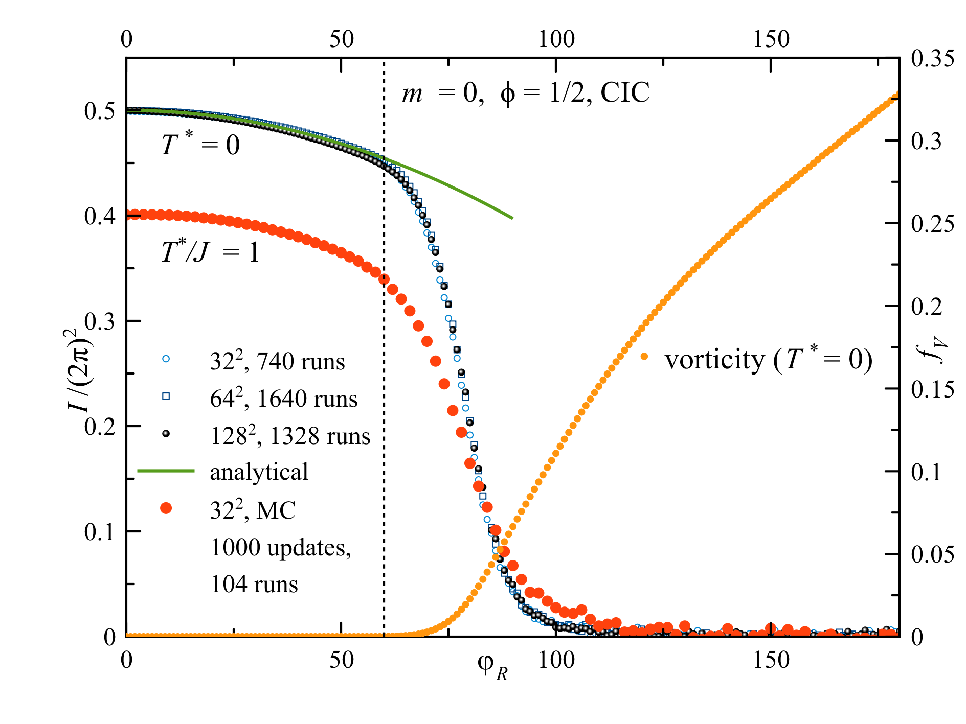
Figure 4: Color online: Disorder dependence of the persistent current and vorticity at different effective temperatures.

In Conclusion, we have proposed a novel system for the study of quantum phase transitions: Josephson junction array wrapped around a cylinder. The dependence of the persistent current on the Josephson and charging energies and on the strength of disorder, computed analytically in the spin wave approximation, agrees well with numerical results. Cases of strong quantum fluctuations and strong disorder have been studied numerically on lattices having over one million sites. Quantum phase transition in the Josephson junction array wrapped around a cylinder is dominated by instantons corresponding to the vortex loops in 2+1 dimensions. Experimental study of such a system would be of great interest.

This work has been supported by the grant No. DE-FG02-93ER45487 funded by the U.S. Department of Energy, Office of Science.

References

- (1) M. Y. Choi, Persistent current and voltage in a ring of Josephson junctions, Physical Review B 48, 15920-15925 (1993).
- (2) K. A. Matveev, A. I. Larkin, and L. I. Glazman, Persistent current in superconducting nanorings, Physical Review Letters 89, 096802-(4) (2002).
- (3) I. M. Pop, I. Protopopov, F. Lecocq, Z. Peng, B. Pannetier, O. Buisson, and W. Guichard, Measurement of the effect of quantum phase-slips in a Josephson junction chain, Nature Physics 6, 589-592 (2010).
- (4) G. Rastelli, I. M. Pop, and F. W . J. Hekking, Quantum phase-slips in Josephson junction rings, Physical Review B 87, 174513-(18) (2013).
- (5) D. A. Garanin and E. M. Chudnovsky, Quantum decay of the persistent current in a Josephson junction ring, Physical Review B 93, 094506-(9) (2016).
- (6) A. D. Zaikin, D. S. Golubev, A. van Otterlo, and G. T. Zimanyi, Quantum phase slips and transport in ultrathin superconducting wires, Physical Review Letters 78, 1552-1555 (1997).
- (7) D. S. Golubev and A. D. Zaikin, Quantum tunneling of the order parameter in superconducting nanowires, Physical Review B 64, 014504-(14) (2001).
- (8) G. Schwiete and Y. Oreg, Persistent current in small superconducting rings, Physical Review Letters 103, 037001-(4) (2009), and references therein.
- (9) A. G. Semenov and A. D. Zaikin, Persistent currents in quantum phase slip rings, Physical Review B 88, 054505-(10) (2013).
- (10) R. M. Bradley and S. Doniach, Quantum fluctuations in chains of Josephson junctions, Physical Review B 30, 1138-1147 (1984).
- (11) S. E. Korshunov, Effect of dissipation on the low-temperature properties of a tunnel-junction chain, Soviet Physics JETP 68, 609-618 (1989).
- (12) E. Chow, P. Delsing, and D. B. Haviland, Length-scale dependence of the superconductor-to-insulator quantum phase transition in one dimension. Physical Review Letters 81, 204-207 (1998).
- (13) See review and references therein: J. E. Mooij, G. Schï¿œn, A. Shnirman, T. Fuse, C. J. P. M. Harmans, H. Rotzinger, and A. H. Verbruggen, Superconductor-insulator transition in nanowires and nanowire arrays, New Journal of Physics 17, 033006-(12) (2015).
- (14) S. L. Sondhi, S. M. Girvin, J. P. Carini, and D. Shahar, Continuous quantum phase transitions, Review of Modern Physics 69, 315-333 (1997).
- (15) S. Sachdev, Quantum Phase Transitions (Cambridge University Press, Cambridge, UK, 2011).
- (16) L. B. Ioffe, M. V. Feigel’man, A. Ioselevich, D. Ivanov, M. Troyer, and G. Blatter, Topologically protected quantum bits using Josephson junction arrays, Nature 415, 503-506 (2002).
- (17) S. Gladchenko, D. Olaya, E. Dupont-Ferrier, B. Dou cot, L. B. Ioffe, and M. E. Gershenson, Superconducting nanocircuits for topologically protected qubits, Nature Physics 5, 48-53 (2009).
- (18) V. E. Manucharyan, J. Koch, L. I. Glazman, and M. H. Devoret, Fluxonium: single Cooper-pair circuit free of charge offsets, Science 326, 113-116 (2009).
- (19) Y.-H. Lin, J. Nelson, and A. M. Goldman, Superconductivity of very thin films: The superconductor-insulator transition, Physica C 514, 130-141 (2015).
- (20) R. Fazio and G. Schön, Physical Review B 43, 5307 (1991).
- (21) Y. Imry, M. Strongin, and C. C. Homes, An inhomogeneous Josephson phase in thin-film and high-Tc superconductors, Physica C 468, 288-293 (2008).
- (22) M. V. Fistul, V. M. Vinokur, and T. I. Baturina, Physical Review Letters 100, 086805 (2008).
- (23) S. V. Syzranov, K. B. Efetov, and B. L. Altshuler, dc conductivity of an array of Josephson junctions in the insulating state, Physical Review Letters 103, 127001-(4) (2009).
- (24) E. M. Chudnovsky, Instanton glass generated by noise in a Josephson junction array, Physical Review Letters 103, 137001-(4) (2009).
- (25) B. A. Bernevig and T. L. Hughes, Topological Insulators and Topological Superconductors, Princeton University Press (Princeton, NJ, 2013).
- (26) M. Lee, M.-S. Choi, and M. Y. Choi, Quantum phase transitions and persistent currents in Josephson-junction ladders, Physical Review B 68, 144506-(11) (2003).
- (27) M. Wallin, E. S. Sørensen, S. M. Girvin, and A. P. Young, Superconductor-insulator transition in two-dimensional dirty boson systems, Physical Review B 49, 12115-12139 (1994).
- (28) K. Kim and D. Stroud, Quantum Monte Carlo study of a magnetic-field-driven two-dimensional superconductor-insulator transition, Physical Review 78, 174517-(16) (2008).
- (29) E. Granato and J. M. Kosterlitz, Quenched disorder in Josephson-junction arrays in a transverse magnetic field, Physical Review B 33, 6533-6536 (R) (1986).
- (30) M. Rubinstein, B. Shraiman, and D. R. Nelson, Two-dimensional XY-magnets with random Dzyaloshinskii-Moriya interactions, Physical Review B 27, 1800-1811 (1983).
- (31) S. E. Korshunov and T. Nattermann, Phase diagram of a Josephson junction array with positional disorder, Physica B 222, 280-286 (1996).
- (32) M. S. Li, T. Nattermann, H. Rieger, and M. Schwartz, Vortex lines in the three-dimensional XY model with random phase shifts, Physical Review B 54, 16026-16031 (1996).
- (33) P. Gupta and S. Teitel, Positional disorder in the fully frustrated Josephson junction array: Random Gaussian Phase Shifts in the Fully Frustrated 2D XY Model, Physical Review Letters 82, 5313-5316 (1999).
- (34) L.-H. Tang and P. Tong, Zero-temperature criticality in the two-dimensional gauge glass model, Physical Review Letters 94, 207204-(4) (2005).
- (35) K. Kim and D. Stroud, Continuous phase transition of a fully frustrated XY model in three dimensions, Physical Review 73, 224504-(10) (2006).
- (36) A. Buzdin, Direct coupling between magnetism and superconducting current in the Josephson junction, Physical Review Letters 101, 107005-(4) (2008).
- (37) F. Konschelle and A. Buzdin, Magnetic moment manipulation by a Josephson current, Physical Review Letters 102, 017001 (2009).
- (38) M. Tinkham, Introduction to Superconductivity (Dover Publications, 2004, ISBN 0-486-43503-2).
- (39) Y. Imry and S.-k. Ma, Random-field instability of the ordered state of continuous symmetry, Physical Review Letters 35, 1399-1401 (1975).
- (40) T. C. Proctor, D. A. Garanin, and E. M. Chudnovsky, Random fields, topology, and the Imry-Ma argument, Physical Review Letters 112, 097201-(4) (2014).