Large $N$ Thirring Matter in Three Dimensions

Abstract

In this paper we calculate properties of the three-dimensional system of $N$ species of fermions at zero temperature and finite chemical potential, with the four-fermionic interaction of the Thirring type. We observe that this model fits consistently into framework of the Landau Fermi liquid theory, and possesses a non-trivial zeroth and first Landau parameters. Our result is derived to all orders of the Thirring coupling constant and to the leading order of the large-$N$ expansion. In particular we solve for the exact current-current correlation function, and show that it exhibits a singular behavior at zero frequency and twice of the Fermi momentum.

1 Introduction

Consider theory of $N$ species of fermions $\psi_{i}$, $i=1,\dots,N$ in the $d$-dimensional space-time. A straightforward way to make this theory dynamical is to switch on a local four-fermionic interaction of the Gross-Neveu $(\bar{\psi}\psi)^{2}$ or the Thirring $(\bar{\psi}\gamma^{\mu}\psi)^{2}$ form Gross:1974jv ; Thirring:1958in . At weak interaction the dimension of the four-fermionic coupling constant is $2-d$. Therefore such an interaction is power-counting non-renormalizable when $d>2$. However the three-dimensional models with a local four-fermionic interaction of the Gross-Neveu and Thirring form are known to be renormalizable and solvable in the large $N$ expansion Parisi:1975 ; Rosenstein:1988pt ; Rosenstein:1988dj ; Rosenstein:1990nm ; Gomez:1990nm ; Hands:1994kb . Such three-dimensional interacting models therefore represent a rather simple exactly solvable fermionic systems which exhibit a non-trivial dynamics.

In this paper we want to discuss a three-dimensional interacting fermionic matter at finite density. The specific model which we choose is the three-dimensional large $N$ Thirring model taken at finite chemical potential for the $U(1)$ particle number. We will solve this model to the leading order in the $1/N$ expansion, and to all orders of the Thirring coupling constant. We will refrain our consideration mostly to the case of zero temperature, and we will set the bare fermionic mass to be zero. In the discussion section we outline the future work and possible interesting generalizations and extensions which can be performed.

One of the phases in which one can find a quantum dense fermionic system is described by the Landau Fermi liquid theory baym2008landau ; abrikosov1975methods ; baym1976landau . This is a finite-density non-condensed state exhibiting a long-lived fermionic quasiparticle excitations. It is defined in the low-temperature regime $T/\mu\ll 1$ in which quasiparticle excitations predominantly exist near the Fermi surface. Interaction of such quasiparticles is characterized by the coupling constants known as the Landau parameters. It has recently been demonstrated that the large-$N$ Chern-Simons-fermion theory provides an example of a microscopic realization of a non-trivial Landau Fermi liquid state Geracie:2015drf . Holographic non-Fermi liquid models are known Lee:2008xf ; Cubrovic:2009ye .

In this paper we show that the dense large-$N$ Thirring model in the low-temperature regime behaves as the Landau Fermi liquid. Our argument is constructed analogously to Geracie:2015drf . First, we calculate the exact fermionic propagator and the four-fermionic scattering amplitude, and use these to calculate the Landau parameters microscopically. Second, we use the Landau Fermi liquid theory expressions for the inverse compressibility and the heat capacity to solve for the Landau parameters. This is possible to do since these thermodynamic quantities can be found by a separate calculation. We show that both these methods give the same values of the Landau parameters.

The relative simplicity of the Thirring model, as compared to the Chern-Simons-fermion model of Geracie:2015drf , allows one to straightforwardly calculate the current-current correlation function at a finite value of the spatial momentum. In the Fermi liquid this correlation function exhibits a singular behavior at zero frequency and twice the Fermi momentum. Experimentally this finite-momentum singularity manifests in a rippling pattern of the charge screening response to insertion of an external charged impurity, known as the Friedel oscillations. A holographic example of a similar oscillatory screening mechanism has recently been obtained in Blake:2014lva . We derive the current-current correlation function for the large $N$ Thirring model and demonstrate explicitly that it exhibits a singular behavior at zero frequency and twice the Fermi momentum. We show that the value of the Fermi momentum is consistent with the Fermi-Dirac quasiparticle distribution and the Luttinger’s theorem.

The paper is organized as follows. In section 2 we briefly summarize the key points of the Landau Fermi liquid theory. In section 3 we formulate the three-dimensional Thirring model at finite chemical potential, and solve for the exact fermionic propagator. In particular this allows one to determine the fermionic distribution function, and calculate the entropy and the heat capacity. From the fermionic distribution function one can read off the value of the Fermi momentum. In section 4 we calculate the current-current correlation function. We show that it exhibits a zero-frequency singular behavior at the value of the momentum, equal to twice the Fermi momentum found in section 3. In section 5 we calculate the values of the Landau parameters from both the microscopic and the thermodynamic perspective, and demonstrate an agreement of both methods. We discuss our results and comment on further work directions in section 6.

2 Landau Fermi liquid theory

In this section we will briefly review some aspects of the Landau Fermi liquid theory. We refer the reader to baym2008landau ; abrikosov1975methods ; baym1976landau ; Geracie:2015drf for the detailed presentation, and in this section we merely outline the very basic statements, in order to make the paper sufficiently self-contained.

The Landau Fermi liquid theory is a low-temperature $T/\mu\ll 1$ theory of a quantum fermionic liquid. Its underlying assumption is that the fundamental low-energy degrees of freedom of the system are long-lived quasiparticles in the vicinity of the Fermi surface. In 2+1 dimensions, which is the case of interest of the present paper, there is no spin degree of freedom, and each quasiparticle state is characterized only by the value of its momentum ${\bf p}$. Define $\varepsilon({\bf p})$ to be an energy of a quasiparticle, and $n({\bf p})$ to be an occupation number.

Interaction of a pair of quasiparticles with momenta ${\bf p}$ and ${\bf p^{\prime}}$ is described by a function $f({\bf p},{\bf p^{\prime}})$, which is introduced in the following way. Suppose occupation numbers of quasiparticles receive a perturbation $\delta n({\bf p})$. In Landau Fermi liquid this results in the following perturbation of the energy of a given quasiparticle:

$$\delta\varepsilon({\bf p})=\int\frac{d^{3}{\bf p^{\prime}}}{(2\pi)^{3}}\,f({\bf p},{\bf p^{\prime}})\,\delta n({\bf p^{\prime}})\,.$$ (1)

The Fermi velocity and the effective mass of a quasiparticle are defined as

$$v_{F}=\frac{\partial\varepsilon({\bf p})}{\partial|{\bf p}|}\Bigg{|}_{|{\bf p}|=p_{F}}\,,\quad\quad m^{\star}=\frac{p_{F}}{v_{F}}\,.$$ (2)

In this paper we will be considering $N$ fermionic flavors, and therefore the observables have an extra index structure:

$$\varepsilon^{i}_{\;\;j}({\bf p}) =\delta^{i}_{j}\,\varepsilon({\bf p})\,,\quad n^{i}_{\;\;j}({\bf p})=\delta^{i}_{j}n\,({\bf p})\,,$$ (3)

$$f^{i\;\;\;\;l}_{\;\;j,\;\;k}({\bf p},{\bf p^{\prime}}) =f^{(d)}({\bf p},{\bf p^{\prime}})\delta^{i}_{j}\delta^{l}_{k}+f^{(e)}({\bf p},{\bf p^{\prime}})\delta^{i}_{k}\delta^{l}_{j}$$ (4)

In the large-$N$ limit the dominant contribution comes from the direct channel, $f^{(d)}$, while the exchange channel, $f^{(e)}$, is suppressed Geracie:2015drf . We therefore will be considering $f^{(d)}=f$. In the low-temperature limit interacting qusiparticles are restricted to the vicinity of the Fermi surface, $|{\bf p}|=|{\bf p^{\prime}}|=p_{F}$. We define $\theta$ to be an angle between ${\bf p}$ and ${\bf p^{\prime}}$, and expand

$$f(\theta)=\frac{1}{\nu(\epsilon_{F})}\left(F_{0}+2\sum_{n=1}^{\infty}F_{n}\cos(n\theta)\right)\,.$$ (5)

The coefficients of expansion, $F_{n}$, $n=0,1,\dots$, are called the Landau parameters. We have defined the density of states on the Fermi surface as

$$\nu(\epsilon_{F})=\frac{Nm^{\star}}{2\pi}\,.$$ (6)

Using the framework outlined above one can derive the values of various observables in terms of the Landau parameters. First of all the quasiparticle effective mass of a relativistic Landau Fermi liquid is given by

$$m^{\star}=\mu\,(1+F_{1})\,.$$ (7)

Quasiparticles with the effective mass $m^{\star}$ obeying the Fermi-Dirac distribution exhibit the following low-temperature behavior of the heat capacity

$$c=\frac{\pi}{6}\,N\,m^{\star}\,T\,.$$ (8)

We will also find useful the following expression for the inverse compressibility

$$\kappa^{-1}=n^{2}\left(\frac{\partial\mu}{\partial n}\right)_{T}=\frac{2\pi n^{2}}{Nm^{\star}}\,(1+F_{0})\,.$$ (9)

Interacting quasiparticles can be described in the framework of quantum field theory. The fermionic propagator, in the Lorentzian signature, near the Fermi surface acquires the form

$$G(p)=\frac{Z}{\omega-v_{F}(|{\bf p}|-p_{F})+i\,\epsilon\,{\rm sgn}(|{\bf p}|-p_{F})}\,\frac{u\otimes\bar{u}}{u^{\dagger}u}\,,$$ (10)

where $u(p)$ is an on-shell spinor describing quasiparticle, and $Z$ is the wave-function renormalization constant. The Landau parameters are calculated as

$$f^{i\;\;\;k}_{\;\;j,\;\;\;l}(\theta)=Z^{2}\lim_{q^{0}\rightarrow 0}\lim_{{\bf q}\rightarrow 0}V^{i\;\;\;k}_{\;\;j,\;\;\;l}(p,k,q)\,,$$ (11)

where the on-shell four-fermionic vertex is

$$V^{i\;\;\;k}_{\;\;j,\;\;\;l}(p,k,q)=\frac{1}{(u^{\dagger}u)^{2}}u_{\alpha}(p+q)u_{\gamma}(k)V^{\alpha\;\;\;\;\gamma}_{\;\;\;\delta,\;\;\;\;\beta}\;{}^{i\;\;\;k}_{\;\;j,\;\;\;l}(p,k,q)\bar{u}^{\beta}(k+q)\bar{u}^{\delta}(p)\,,$$ (12)

and the one-particle irreducible four-fermionic amplitude is given by

$$V^{\alpha\;\;\;\;\gamma}_{\;\;\;\delta\;\;\;\;\beta}\;{}^{i\;\;\;k}_{\;\;j\;\;\;l}(p,k,q)=\left\langle\bar{\psi}^{\alpha i}(-p-q)\bar{\psi}^{\gamma k}(-k)\psi_{\delta l}(p)\psi_{\beta j}(k+q)\right\rangle_{1PI}\,.$$ (13)

3 Thirring model

In this paper we study the system of $N$ massless Dirac fermions interacting via the four-fermionic Thirring coupling. We will be working in the Euclidean space, with $x^{1,2}$ being the space coordinates, and $x^{3}$ being the Euclidean time coordinate. We consider the model at finite chemical potential $\mu$ for the $U(1)$ particle number current $j^{\mu}=\bar{\psi}^{n}\gamma^{\mu}\psi_{n}$. We will mostly be considering the system at zero temperature. The Lagrangian is given by

$${\cal L}=\bar{\psi}^{n}\gamma^{\mu}\partial_{\mu}\psi_{n}+\mu\,\bar{\psi}^{n}\gamma^{3}\psi_{n}+\frac{1}{2\sigma^{2}N}\,\bar{\psi}^{n}\gamma^{\mu}\psi_{n}\,\bar{\psi}^{m}\gamma_{\mu}\psi_{m}\,.$$ (14)

Here $\sigma^{2}$ has a dimension of mass, and the case of free fermions corresponds to taking the limit $\sigma^{2}\rightarrow\infty$. The conjugate spinor in the Euclidean space is $\bar{\psi}=\psi^{\dagger}$. An extra prefactor of $1/2$ in (14) is introduced for further convenience. In the case $\sigma^{2}>0$ the interaction is repulsive, while in the case $\sigma^{2}<0$ the interaction is attractive.

The model (14) is exactly solvable in the large-$N$ limit. In this paper we are interested in the solution at the leading order in the $1/N$ expansion. Let us begin by solving for the exact fermionic propagator,

$$\langle\psi_{m}(p)\bar{\psi}^{n}(-q)\rangle=\delta_{m}^{n}G(p)(2\pi)^{3}\delta(p-q)\,,$$ (15)

We will be looking for the solution of the form

$$G(p)=\frac{1}{i\tilde{p}_{\mu}\gamma^{\mu}+\Sigma(p)}\,,$$ (16)

where $\tilde{p}_{\mu}=p_{\mu}-i\mu\delta_{\mu,3}$. The fermionic self-energy $\Sigma(p)$ satisfies the Schwinger-Dyson equation,

$$\Sigma(p)=\frac{1}{\sigma^{2}}\gamma^{\mu}\int\frac{d^{3}r}{(2\pi)^{3}}{\rm Tr}(G(r)\gamma_{\mu})\,.$$ (17)

It can be derived in the path integral framework, as well as from the following diagramatic consideration:

It is clear from equation (17) that the solution is momentum independent, $\Sigma(p)\equiv{\rm const}$, which is the consequence of a contact nature of the Thirring interaction. After regularizing the integrals over $r_{3}$ and $r_{s}=\sqrt{r_{1}^{2}+r_{2}^{2}}$, we arrived at

$$\Sigma_{1} =0\,,\quad\quad\Sigma_{2}=0\,,\quad\quad\Sigma_{3}=-\frac{\hat{\mu}^{2}}{4\pi\sigma^{2}}\,,$$ (18)

where

$$\hat{\mu}=\mu+\Sigma_{3}\,.$$ (19)

Therefore the exact fermionic propagator is the same as the free fermionic propagator, but with the renormalized chemical potential (19),

$$G(p)=\frac{1}{i\hat{p}_{\mu}\gamma^{\mu}}\,,\quad\quad\hat{p}_{\mu} =p_{\mu}-i\hat{\mu}\delta_{\mu,3}\,.$$ (20)

From the exact fermionic propagator one can derive the distribution function for fermionic states in the momentum space (quasiparticle occupation number),

$$n({\bf p})=\int\frac{dp_{3}}{2\pi}\int\frac{d^{3}q}{(2\pi)^{3}}\left\langle\bar{\psi}^{n}(q)\gamma^{3}\psi_{n}(p)\right\rangle=N\,\theta(\hat{\mu}-|{\bf p}|)\,.$$ (21)

This distribution function indicates a presence of the Fermi surface, with the Fermi momentum given by

$$p_{F}=\hat{\mu}\,.$$ (22)

Knowing the distribution function one can determine the density of fermions

$$n=-\frac{\partial\log Z}{\partial\mu}=\int\frac{d^{2}p}{(2\pi)^{2}}n({\bf p})=N\,\frac{\hat{\mu}^{2}}{4\pi}\,.$$ (23)

Notice that the expression (23) is derived without explicit use of expression for the free energy, and is a manifestation of the Luttinger’s theorem for fermions at zero temperature, with the Fermi momentum $p_{F}=\hat{\mu}$.

We have therefore demonstrated that zero-temperature occupation number for fermionic states is given by a step function, and we have identified the Fermi momentum by the location of the step. In the next section we demonstrate how a singular structure at zero frequency and twice of the Fermi momentum is manifested in the current-current correlation function.

In this paper we are mostly interested in the case of zero temperature. However one of the hallmarks of the Landau Fermi liquid is a linear temperature dependence of the low-temperature heat capacity (8). Therefore in the remaining part of this section we briefly outline derivation of the the fermionic propagator and the occupation number at finite temperature.

The Schwinger-Dyson equation at finite temperature is

$$\Sigma(p)=\frac{1}{\sigma^{2}}\gamma^{\mu}\,\frac{1}{\beta}\,\sum_{n}\,\int\frac{d^{2}r}{(2\pi)^{2}}{\rm Tr}(G(r)\gamma_{\mu})\Bigg{|}_{\tilde{r}_{3}=2\pi(n+1/2)/\beta-i\mu}\,.$$ (24)

The solution for $\Sigma_{1,2}$ is again trivial, while $\Sigma_{3}$ is a constant, shifting the chemical potential, $\hat{\mu}=\mu+\Sigma_{3}$. Regularizing the sum over $n$, and the integral over $r_{s}$ one can obtain the finite-temperature equation for $\Sigma_{3}$. The precise form of this equation is not essential for our present purposes and will be derived elsewhere.

The occupation number can again be calculated from the fermionic propagator,

$$n({\bf p}) =\frac{1}{\beta}\,\sum_{n}\,{\rm Tr}\left(\gamma^{3}G\left(p_{3}=\frac{2\pi\left(n+\frac{1}{2}\right)}{\beta}-i\mu,{\bf p}\right)\right)$$ (25)

$$=\frac{1}{2}\left(\tanh\left(\frac{1}{2}\beta(p_{s}+\hat{\mu})\right)-\tanh\left(\frac{1}{2}\beta(p_{s}-\hat{\mu})\right)\right)\,,$$ (26)

which is the Fermi-Dirac distribution of massless Dirac fermion with energy $E=p_{s}$ at the chemical potential $\hat{\mu}$. Knowing the distribution function one can determine the entropy and the heat capacity of the system,

$$s=\frac{\pi}{6}\,N\,\hat{\mu}\,T\,,\qquad c=\frac{\pi}{6}\,N\,\hat{\mu}\,T\,.$$ (27)

This agrees with the Landau Fermi liquid expression (8), provided the quasiparticle effective mass is $m^{\star}=\hat{\mu}$.

4 Current-current correlator

In the previous section we showed that fermionic distribution function of the zero-temperature Thirring model at finite chemical potential $\mu$ is a step function, with the step located at the momentum (22). This is what we expect to see when a sharp Fermi surface is formed. In this section we want to provide an independent verification of existence of the Fermi surface.

One can detect the Fermi surface experimentally by observing response of the system to an external charged impurity. Due to the Fermi surface the charge screening mechanism will exhibit a rippling pattern, which can be traced back to a singular structure of the current-current correlation function at zero frequency and finite momentum. In this section we perform a calculation of the current-current correlation function in the Thirring model, and show that it is singular at zero frequency and the momentum equal to twice of the Fermi momentum (22), as it is expected in Fermi liquids.

Consider the global $U(1)$ current, $j^{\mu}(x)=\bar{\psi}^{m}(x)\gamma^{\mu}\psi_{m}(x)$. Corresponding bi-fermionic vertex is

$$(T^{\mu})^{\alpha}_{\;\;\beta}(p,q)\,\delta^{n}_{m}=\langle\bar{\psi}_{m}^{\alpha}(p+q)\psi_{\beta}^{n}(p)j^{\mu}(-q)\rangle\,.$$ (28)

We propose the following ansatz to incorporate the spinor structure of the vertex

$$T^{\mu}=T^{\mu}_{\;\;\nu}\gamma^{\nu}\,.$$ (29)

This vertex satisfies the Schwinger-Dyson equation

$$T^{\mu}_{\;\;\nu}(q)\gamma^{\nu}=\gamma^{\mu}+\frac{1}{\sigma^{2}}\gamma^{\nu}\,T^{\mu\lambda}(q)\int\frac{d^{3}r}{(2\pi)^{3}}\,{\rm Tr}\,(\gamma_{\nu}G(r+q)\gamma_{\lambda}G(r))\,,$$ (30)

which diagramatically is depicted as (the large black vertex stands for four-fermionic coupling, the small black vertex stands for free contraction point, the internal fermionic lines are full propagators)

Here we have noticed that once again the momentum dependence is only on the total momentum $q$. This in turn leaves us with just an algebraic equation

$$T^{\mu}_{\;\;\nu}=\delta^{\mu}_{\;\;\nu}-\frac{1}{\sigma^{2}}T^{\mu}_{\;\;\lambda}v^{\lambda}_{\;\;\nu}\,,$$ (31)

where we have defined

$$v_{\mu\nu}={\rm Tr}(\gamma_{\mu}\gamma_{\alpha}\gamma_{\nu}\gamma_{\beta})\,\int\frac{d^{3}r}{(2\pi)^{3}}\frac{1}{\hat{r}^{2}(\hat{r}+q)^{2}}\hat{r}^{\alpha}(\hat{r}+q)^{\beta}\,.$$ (32)

The solution is

$$T=\sigma^{2}(\sigma^{2}\,I+v)^{-1}\,.$$ (33)

The current-current correlator can then be straightforwardly calculated,

$$\langle j^{\nu}(-q)j^{\mu}(q)\rangle =N\,T^{\mu}_{\;\;\lambda}(q)\int\frac{d^{3}r}{(2\pi)^{3}}\,{\rm Tr}\,(\gamma^{\nu}G(r+q)\gamma^{\lambda}G(r))$$ (34)

$$=-(T\,v)^{\mu\nu}$$ (35)

$$=-N\,\sigma^{2}((\sigma^{2}\,I+v)^{-1}\,v)^{\mu\nu}\,.$$ (36)

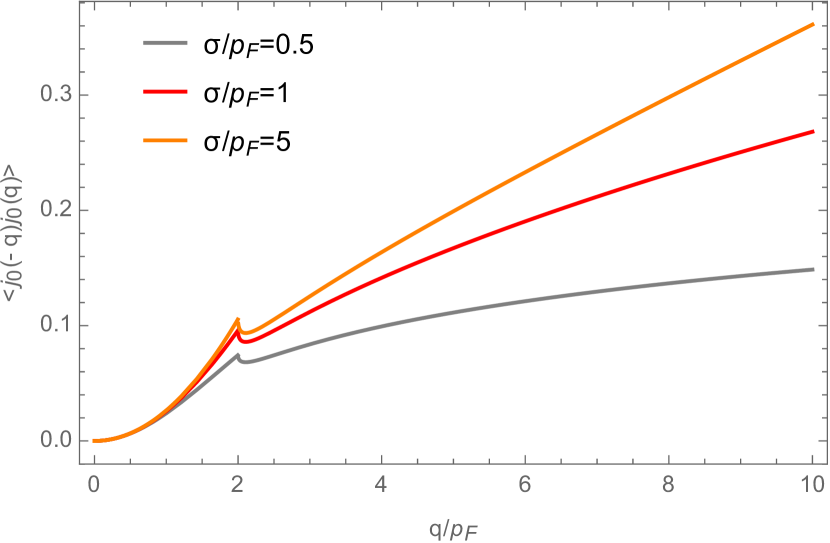
Figure 1: The real part of the density-density correlation function $\left\langle j_{0}(0,-q)j_{0}(0,q)\right\rangle$, at various values of the coupling constant $\sigma$. The imaginary part identically vanishes at zero frequency.

It requires some work to calculate $v_{\mu\nu}$ at non-zero momentum, however when $q_{3}=0$ the derivation somewhat simplifies, but still remains cumbersome. We provide the details of its calculation in Appendix A. The most important feature is the singular structure of the correlation function at $q_{s}=2p_{F}=2\hat{\mu}$. We plot the result at various values of the coupling constant in figure 1. At finite value of the coupling $\sigma$ we obtain the asymptotic expression (remember $\sigma^{2}$ has dimension of mass)

$$\frac{1}{N}\,\left\langle j_{0}(0,-{\bf q})j_{0}(0,{\bf q})\right\rangle\simeq\sigma^{2}-\frac{32\sigma^{4}}{q_{s}}+{\cal O}\left(1/q_{s}^{2}\right)\,.$$ (37)

On the other hand if the free limit $\sigma\rightarrow\infty$ is taken first, then the asymptotic behavior is

$$\frac{1}{N}\,\left\langle j_{0}(0,-{\bf q})j_{0}(0,{\bf q})\right\rangle_{\sigma\rightarrow\infty}\simeq\frac{q_{s}}{32}+\frac{\mu}{16}+{\cal O}\left(1/q_{s}\right)\,.$$ (38)

We also calculate

$$\frac{1}{N}\,\lim_{q_{s}\rightarrow 0}\left\langle j_{\parallel}(0,-{\bf q})j_{\parallel}(0,{\bf q})\right\rangle=\frac{p_{F}^{2}}{4\pi\mu}$$ (39)

which then can be substituted into the Kubo formula to give the following expression for the AC conductivity at low frequency

$$\sigma(\omega)=N\,\frac{p_{F}^{2}}{4\pi\mu}\frac{1}{-i\omega}\,.$$ (40)

This agrees with the Drude model, with infinitely long-lived charge carriers with the density given by (23).

5 Landau parameters

In the Landau Fermi liquid theory the interaction of quasiparticles on the Fermi surface can be described by the Landau parameters, as we briefly reviewed in section 2. In the first part of this section we derive the Landau parameters for the Thirring model from microscopic considerations. We begin by solving the Schwinger-Dyson equation for the fermionic four-point function (13). Knowing the on-shell fermionic states on the Fermi surface, we subsequently derive the amplitude (12), and the quasiparticle interaction function (11).

Thermodynamic observables in the Landau Fermi liquid theory can be expressed in terms of the Landau parameters. As reviewed in section 2, the heat capacity and the inverse compressibility can be calculated using (8), (9). The reverse of this procedure expresses the Landau parameters in terms of the known thermodynamic observables. In the second part of this section we show that such a method gives the values of the Landau parameters agreeing with the microscopic result.

5.1 Four-fermionic vertex

Consider the four-fermionic one-particle irreducible amplitude in the direct channel

$$V^{\alpha\;\;\;\;\gamma}_{\;\;\delta\;\;,\;\;\beta}(q)\,\delta^{i}_{l}\,\delta^{j}_{k}=\left\langle\bar{\psi}^{\alpha i}(-p-q)\bar{\psi}^{\gamma k}(-k)\psi_{\delta l}(p)\psi_{\beta j}(k+q)\right\rangle_{1PI}$$ (41)

It satisfies the Schwinger-Dyson equation, which in the large-$N$ limit is written as

$$V^{\alpha\;\;\;\;\gamma}_{\;\;\delta\;\;,\;\;\beta}(q)=\frac{1}{\sigma^{2}}(\gamma^{\mu})^{\alpha}_{\;\;\delta}(\gamma_{\mu})^{\gamma}_{\;\;\beta}+\frac{1}{\sigma^{2}}(\gamma^{\mu})^{\alpha}_{\;\;\delta}\int\frac{d^{3}r}{(2\pi)^{3}}{\rm Tr}_{1}\left(G(r)\gamma_{\mu}G(r+q)V^{\;\;\;\;\gamma}_{\;\;\;\;,\;\;\beta}(q)\right)$$ (42)

The pairs of indices $(\alpha,\delta)$ and $(\gamma,\beta)$ are separated by comma in the notation for the vertex, and belong to different terms in the direct product of spinor structure. Diagramatically the Schwinger-Dyson equation (42) looks like

Here we have lightened up the picture, removing the superfluous momentum labels where their placement is clear. The $r$ and $r+q$ internal fermionic propagators are the full fermionic propagators.

In the case of general momentum $q$ one would consider the following ansazt for the spinor structure of the vertex

$$V^{\alpha\;\;\;\;\gamma}_{\;\;\delta\;\;,\;\;\beta}(q)=(\gamma_{\mu})^{\alpha}_{\;\;\delta}(\gamma_{\nu})^{\gamma}_{\;\;\beta}A^{\mu\nu}(q)\,,$$ (43)

and therefore the SD equation takes the form

$$(\gamma_{\mu})^{\alpha}_{\;\;\delta}(\gamma_{\nu})^{\gamma}_{\;\;\beta}A^{\mu\nu}(q)=\frac{1}{\sigma^{2}}(\gamma^{\mu})^{\alpha}_{\;\;\delta}(\gamma_{\mu})^{\gamma}_{\;\;\beta}-\frac{1}{\sigma^{2}}(\gamma^{\mu})^{\alpha}_{\;\;\beta}v_{\nu\mu}(q)A^{\nu}_{\;\;\lambda}(q)(\gamma^{\lambda})^{\gamma}_{\;\;\beta}\,,$$ (44)

where we have used (32). For the purpose of calculating the Landau parameters we are interested in the four-fermionic vertex at zero momentum, $q=0$. In that case

$$v_{\mu\nu}(q=0)=\frac{\hat{\mu}}{4\pi}(\delta_{\mu,1}\delta_{\nu,1}+\delta_{\mu,2}\delta_{\nu,2})$$ (45)

The SD equation therefore has the solution

$$A_{\mu\nu}(q=0)={\rm diag}\,\left(\frac{1}{\sigma^{2}+\frac{\hat{\mu}}{4\pi}},\,\frac{1}{\sigma^{2}+\frac{\hat{\mu}}{4\pi}},\,\frac{1}{\sigma^{2}}\right)\,.$$ (46)

5.2 Microscopic derivation of the Landau parameters

The on-shell particle state $u(p)$ satisfies the Dirac equation

$$\hat{p}_{\mu}\gamma^{\mu}u(p)=0\,,$$ (47)

and therefore it obeys the mass-shell condition

$$(p_{3}-i\mu-i\Sigma_{3})^{2}+p_{s}^{2}=0\,.$$ (48)

The Euclidean energy is $\varepsilon=\tilde{p}_{3}=p_{3}-i\mu$. On the Fermi surface the energy is $\varepsilon=\varepsilon_{F}=-i\mu$, and the momentum is $p_{F}=\hat{\mu}$. Dirac equation (47) on the Fermi surface takes the form

$$\left({-i\atop e^{i\theta_{p}}}\;{e^{-i\theta_{p}}\atop i}\right)u(p)=0\,.$$ (49)

The solution is

$$u(p)=\left({-ie^{-i\theta_{p}/2}\atop e^{i\theta_{p}/2}}\right)\,.$$ (50)

Now we switch to the Lorentzian signature and expand the fermionic propagator near the Fermi surface

$$G(p)=-\frac{i\hat{p}_{\mu}\gamma^{\mu}}{\hat{p}^{2}}\simeq\frac{1}{\omega-\,(|{\bf p}|-p_{F})}\frac{u\otimes\bar{u}}{u^{\dagger}u}\,,$$ (51)

which has the form of (10), with the wave-function remormalization

$$Z=1\,.$$ (52)

and the Fermi velocity

$$v_{F}=1\,.$$ (53)

Consequently the quasiparticle effective mass is given by

$$m^{\star}=\frac{p_{F}}{v_{F}}=\hat{\mu}\,.$$ (54)

The quasiparticle interaction function $f(\theta)$ can be derived microscopically from the one-particle-irreducible scattering amplitude, (11), (12). Using the solution for $V^{\alpha\;\;\;\;\gamma}_{\;\;\delta\;\;,\;\;\beta}(0)$, and the expression (50) for the on-shell fermionic state, we obtain

$$f(\theta)=\frac{1}{\sigma^{2}}-\frac{1}{\sigma^{2}+\frac{\hat{\mu}}{4\pi}}\,\cos\theta\,,$$ (55)

where $\theta=\theta_{p}-\theta_{k}$.

The Landau parameters can now be extracted using the expansion (5). We expresse the answer in terms of the Thirring coupling constant $\sigma$ and the Fermi momentum $\hat{\mu}$,

$$F_{0} =\frac{\hat{\mu}}{2\pi\sigma^{2}}\,,$$ (56)

$$F_{1} =-\frac{\hat{\mu}}{4\pi\sigma^{2}+\hat{\mu}}\,.$$ (57)

5.3 Thermodynamic derivation of the Landau parameters

One can derive the Landau parameters $F_{0}$, $F_{1}$, provided the inverse compressibility and the heat capacity are known. We know that the charge density $n$ is given by (23), which allows us to calculate the inverse compressibility (9). Due to $m^{\star}=\hat{\mu}=\mu+\Sigma_{3}$, we obtain

$$F_{0} =N\,\frac{\hat{\mu}}{2\pi}\frac{\partial\mu}{\partial n}-1=\left(1-\frac{\partial\hat{\mu}}{\partial\mu}\right)/\frac{\partial\hat{\mu}}{\partial\mu}\,.$$ (58)

We notice that this is the same as the expression (56) derived from microscopic considerations, once we observe that

$$\left(1-\frac{\partial\hat{\mu}}{\partial\mu}\right)/\frac{\partial\hat{\mu}}{\partial\mu}=\frac{\hat{\mu}}{2\pi\sigma^{2}}\,,$$ (59)

as follows from differentiating w.r.t. $\mu$ of the expression, obtained from equations (18), (19)

$$\frac{\hat{\mu}^{2}}{4\pi}+\sigma^{2}\hat{\mu}-\sigma^{2}\mu=0\,.$$ (60)

The heat capacity of the Landau Fermi liquid is given by the expression (8). Comparing it with the expression (27) for the Thirring model we conclude that $m^{\star}=\hat{\mu}$, in agreement to the value (54) we obtained from the fermionic propagator. After some transformations using the Landau Fermi liquid expression (7) and the relations (18), (19) we conclude that the $F_{1}$ is given by the expression (57), in agreement with the microscopic derivation of the previous subsection.

5.4 Solving for the Landau parameters

The gap equation (60) is solved by

$$\hat{\mu}=\mu\,\frac{\sqrt{1+t}-1}{t/2}\,,$$ (61)

where we have denoted

$$t=\frac{\mu}{\pi\sigma^{2}}\,.$$ (62)

The fermionic density is then given by

$$n(t)=N\,\frac{\mu^{2}}{\pi\,t^{2}}\,(\sqrt{1+t}-1)^{2}\,.$$ (63)

The Landau parameters are

$$F_{0}(t) =\sqrt{1+t}-1\,,$$ (64)

$$F_{1}(t) =-\frac{1}{t}\,(\sqrt{1+t}-1)^{2}\,.$$ (65)

We plot these for the attractive and repulsive interactions in figures 3, 3.

The free theory limit is $t\rightarrow 0$. In the case of attractive interaction we have $t<0$, in the case of repulsive interaction it is $t>0$. The theory always has a real-valued solution for $\hat{\mu}$ when interaction is repulsive. When interaction is attractive, the solution is only valid for $t\in[-1,0]$, putting an upper threshold $t=-1$ on the possible interaction strength at which the Fermi liquid state can exist. Notice the density $n(t)$ does not vanish at the threshold point $t=-1$, indicating that the system actually goes through a phase transition at this point, to a different finite-density state. This is not unexpected for a three-dimensional model with local four-fermionic interaction, since it is known that a finite-density Gross-Neveu model exhibits a deconfinement phase transition at certain value of the chemical potential Rosenstein:1988dj ; Rosenstein:1990nm . It would be interesting to derive the free energy for the Thirring model, at finite temperature and chemical potential, and map the corresponding phase struture.

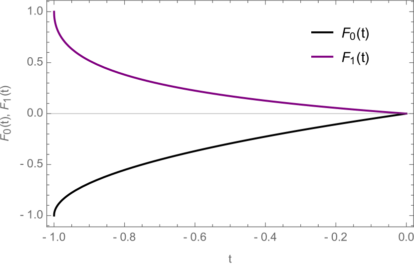
Figure 2: The Landau parameters in the Thirring model with attractive interactions ($\sigma^{2}<0$) in dependence on the $t=\mu/(\pi\sigma^{2})$, taking values between the free point $t=0$ and the threshold point $t=-1$ of the Fermi liquid phase.

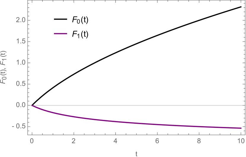
Figure 3: The Landau parameters in the Thirring model with repulsive interactions ($\sigma^{2}>0$) in dependence on the $t=\mu/(\pi\sigma^{2})$, taking values between the free point $t=0$ and the infinitely strongly coupled regime $t\gg 1$.

6 Discussion

In this paper we considered the large $N$ limit of the three-dimensional Thirring model of massless fermions at finite density. Such a model provides a simple example of an interacting fermionic system, and we have shown that its low-temperature dynamics consistently fits into the framework of the Landau Fermi liquid with a non-trivial zeroth and first Landau parameters. We have argued that the system exhibits a sharp Fermi surface at zero temperature by calculating the current-current correlation function and demonstrating that it has a singular structure at zero frequency and a finite momentum, equal to twice of the Fermi momentum.

An immediate generalization of the model considered in this paper is achieved by switching on a finite temperature. The Landau Fermi liquid theory is defined in the low-temperature range, $T/\mu\ll 1$. Unlike the situation of the Chern-Simons-matter theories, introduction of temperature into the Thirring model is relatively simple, because in the absence of gauge interaction one does not have to worry about holonomy of the gauge field along the temporal circle. It is interesting to calculate the current-current correlation function at finite value of the temperature, and study its singular structure.

Another straightforward calculation which can be done is the large-$N$ free energy and the associated phase structure. Furthermore, it would be interesting to repeat the analyses of this paper for the three-dimensional massive fermionic model with the Gross-Neveu interaction, which exhibits a second order phase transition Rosenstein:1988dj ; Rosenstein:1990nm . It would be interesting to observe the associated behavior of the Landau parameters and to follow the fate of the Friedel oscillations across the point of the superconducting phase transition.

Appendix A Derivation of the $v$ matrix

In this appendix we derive the $v_{\mu\nu}$ matrix (32)

$$v_{\mu\nu}={\rm Tr}(\gamma_{\mu}\gamma_{\alpha}\gamma_{\nu}\gamma_{\beta})\,\int\frac{d^{3}r}{(2\pi)^{3}}\frac{1}{\hat{r}^{2}(\hat{r}+q)^{2}}\hat{r}^{\alpha}(\hat{r}+q)^{\beta}\,.$$ (66)

Let us introduce the $u_{\alpha\beta}$ matrix

$$u^{\alpha\beta}=\int\frac{d^{3}r}{(2\pi)^{3}}\frac{1}{\hat{r}^{2}(\hat{r}+q)^{2}}\hat{r}^{\alpha}(\hat{r}+q)^{\beta}\,,$$ (67)

which then allows us to express

$$v_{\mu\nu}=2(u_{\mu\nu}+u_{\nu\mu}-{\rm Tr}\,u\,g_{\mu\nu})\,.$$ (68)

We are interested in the calculation at $q_{3}=0$. The calculation therefore reduces to deriving the following integrals:

$$S_{\mu}(q_{3}=0) =\int\frac{d^{3}r}{(2\pi)^{3}}\frac{\hat{r}_{\mu}}{\hat{r}^{2}(\hat{r}+q)^{2}}\,,$$ (69)

$$S_{\mu\nu}(q_{3}=0) =\int\frac{d^{3}r}{(2\pi)^{3}}\frac{\hat{r}_{\mu}\hat{r}_{\nu}}{\hat{r}^{2}(\hat{r}+q)^{2}}\,,$$ (70)

in terms of which

$$u^{\alpha\beta}(q_{3}=0)=S^{\alpha\beta}(q_{3}=0)+S^{\alpha}(q_{3}=0)q^{\beta}\,.$$ (71)

For simplicity of notation in this appendix we omit hats on top of $\hat{\mu}$.

Let us derive the $S_{\mu}$ first. Introducing the Feynman parameter we obtain

$$S_{\mu}(q_{3}=0)=\int_{0}^{1}dx\,\int\frac{d^{3}r}{(2\pi)^{3}}\,\frac{\tilde{r}_{\mu}}{[\tilde{r}_{3}^{2}+a^{2}]^{2}}\,,$$ (72)

where $b^{2}=(r+xq)_{s}^{2}+x(1-x)q_{s}^{2}$. First integrating over $r_{3}$ we notice that

$$S_{3}(q_{3}=0)=0\,.$$ (73)

Consider $\mu=i$ to be a spatial polarization, and make the change $r_{i}\rightarrow r_{i}-x\,q_{i}$ of the integrated momentum,

$$S_{i}(q_{3}=0) =-q_{i}\,\int_{0}^{1}dx\,x\,\int\frac{d^{3}r}{(2\pi)^{3}}\,\frac{1}{[\tilde{r}_{3}^{2}+a^{2}]^{2}}$$ (74)

$$=-\frac{q_{i}}{8\pi}\,\int_{0}^{1}dx\,x\,\int\frac{d^{2}r}{(2\pi)^{2}}\,\int_{\sqrt{x(1-x)}q_{s}}^{\Lambda+xq_{s}\cos\theta}\frac{da}{a^{2}}\,\theta(a-\mu)\,,$$ (75)

where $a^{2}=r_{s}^{2}+x(1-x)q_{s}^{2}$.

Here we have also noticed that on should generally take into account that if the $r_{s}$ integral is divergent then an extra subtlety appears in regularization of the divergence. Suppose we choose a cutoff scale, $r_{s}<\Lambda$. Then after the change of the variables the cutoff scale is $a<\Lambda+xq_{s}\cos\theta+{\cal O}(1/\Lambda)$, where $\theta$ is an angle between ${\bf r}$ and ${\bf q}$. Due to the presence of $\cos\theta$, the shift $xq_{s}\cos\theta$ of the cutoff scale usually vanishes after integration over $\theta$, and in all the integrals below it actually ends up having no contribution.

Denote $x_{1,2}$ to be solutions of equation $x(1-x)q_{s}^{2}=\mu^{2}$. Then

$$S_{i}(q_{3}=0) =-\frac{q_{i}}{8\pi}\,\int_{0}^{1}dx\,x\,\int_{\mu}\frac{da}{a^{2}}\,\theta(2\mu-q_{s})$$ (76)

$$-\frac{q_{i}}{8\pi}\left(\left(\int_{0}^{x_{1}}dx\,x+\int_{x_{2}}^{1}dx\,x\right)\frac{1}{\mu}+\int_{x_{1}}^{x_{2}}dx\,x\frac{1}{q_{s}\sqrt{x(1-x)}}\right)\,\theta(q_{s}-2\mu)$$

$$=-\frac{q_{i}}{16\pi\mu}+\frac{1}{8\pi}\left(\frac{\sqrt{q_{s}^{2}-4\mu^{2}}}{2\mu}-\cos^{-1}\left(\frac{2\mu}{q_{s}}\right)\right)\,\theta(q_{s}-2\mu)\,.$$ (77)

Therefore for the polarizations longitudinal and transverse w.r.t. ${\bf q}$ we obtain

$$S_{\parallel}(q_{3}=0) =-\frac{q_{s}}{16\pi\mu}+\frac{1}{16\pi\mu}\left(\sqrt{q_{s}^{2}-4\mu^{2}}-2\mu\,\cos^{-1}\left(\frac{2\mu}{q_{s}}\right)\right)\,\theta(q_{s}-2\mu)\,,$$ (78)

$$S_{\perp}(q_{3}=0) =0\,.$$ (79)

Calculation of the tensor $S_{\mu\nu}$ is performed analogously. First of all we notice that

$$S_{3i}(q_{3}=0) =0$$ (80)

$$S_{33}(q_{3}=0) =-\frac{\mu}{8\pi}+\left(\frac{\mu}{16\pi q_{s}}\sqrt{q_{s}^{2}-4\mu^{2}}-\frac{q_{s}}{32\pi}\cos^{-1}\frac{2\mu}{q_{s}}\right)\theta(q_{s}-2\mu)\,.$$ (81)

We subseqeuntly find

$$S_{ij}(q_{3}=0) =\frac{1}{8\pi}\,\int_{0}^{1}dx\int\frac{d\theta}{2\pi}\int_{\sqrt{x(1-x)}q_{s}}^{\Lambda+xq_{s}\cos\theta}\frac{da}{a^{2}}\,\theta(a-\mu)\,(r_{i}r_{j}+x^{2}q_{i}q_{j})\,.$$ (82)

which in components is given by

$$S_{\parallel\parallel}(q_{3}=0) =\frac{q_{s}^{2}-2\mu^{2}}{32\pi\mu}+\frac{2\mu q_{s}\cos^{-1}\left(\frac{2\mu}{q_{s}}\right)-q_{s}\sqrt{q_{s}^{2}-4\mu^{2}}}{32\pi\mu}\,\theta(q_{s}-2\mu)\,,$$ (83)

$$S_{\perp\perp}(q_{3}=0) =-\frac{q_{s}^{2}+6\mu^{2}}{96\pi\mu}+\frac{\sqrt{q_{s}^{2}-4\mu^{2}}\left(8\mu^{2}+q_{s}^{2}-6\mu^{2}\cos^{-1}\left(\frac{2\mu}{q_{s}}\right)\right)}{96\pi\mu q_{s}}\,\theta(q_{s}-2\mu)$$ (84)

$$S_{\parallel\perp}(q_{3}=0) =0\,.$$ (85)

Notice that all the integrals are real-valued at $q_{3}=0$. This can alternatively be seen by working in the Lorentzian signature, where the fermionic propagator at finite chemical potential attains the form

$$\frac{1}{-p_{3}^{2}+p_{s}^{2}}\rightarrow\frac{1}{(p_{3}+p_{s}-i\epsilon)(p_{3}-p_{s}+i\epsilon{\rm sgn}(p_{s}-\hat{\mu}))}\,.$$ (86)

Using this propagator in the loop integral at zero frequency one notices that the resulting integrals over spatial components of the total momentum are to be understood in the principal value sense, and can be seen to be real-valued.

For the density-density correlation function, restoring $\mu\rightarrow\hat{\mu}$, we obtain

$$\frac{1}{N}\,\left\langle j_{3}(-q)j_{3}(q)\right\rangle=\frac{q_{s}^{2}\sigma^{2}\,\theta(2\hat{\mu}-q_{s})}{12\pi\hat{\mu}\sigma^{2}+q_{s}^{2}}$$ (87)

$${+}\frac{\sigma^{2}\left(4q_{s}^{3}{-}4q_{s}^{2}\sqrt{q_{s}^{2}{-}4\hat{\mu}^{2}}{-}2\hat{\mu}^{2}\sqrt{q_{s}^{2}{-}4\hat{\mu}^{2}}+3\hat{\mu}\left(2\hat{\mu}\sqrt{q_{s}^{2}{-}4\hat{\mu}^{2}}{+}q_{s}^{2}\right)\cos^{-1}\left(\frac{2\hat{\mu}}{q_{s}}\right)\right)\,\theta(q_{s}{-}2\hat{\mu})}{4q_{s}^{3}{-}4q_{s}^{2}\sqrt{q_{s}^{2}{-}4\hat{\mu}^{2}}{-}2\hat{\mu}^{2}\sqrt{q_{s}^{2}{-}4\hat{\mu}^{2}}{+}3\hat{\mu}\left(2\hat{\mu}\sqrt{q_{s}^{2}{-}4\hat{\mu}^{2}}{+}q_{s}^{2}\right)\cos^{-1}\left(\frac{2\hat{\mu}}{q_{s}}\right){+}48\pi\hat{\mu}q_{s}\sigma^{2}}\,.$$

References

- (1) D. J. Gross and A. Neveu, Dynamical Symmetry Breaking in Asymptotically Free Field Theories, Phys. Rev. D10 (1974) 3235.
- (2) W. E. Thirring, A Soluble relativistic field theory?, Annals Phys. 3 (1958) 91–112.
- (3) G. Parisi, The Theory of Nonrenormalizable Interactions. 1. The Large N Expansion, Nucl. Phys. B. 100 (1975) 368–388.
- (4) B. Rosenstein, B. J. Warr, and S. H. Park, The Four Fermi Theory Is Renormalizable in (2+1)-Dimensions, Phys. Rev. Lett. 62 (1989) 1433–1436.
- (5) B. Rosenstein, B. J. Warr, and S. H. Park, Thermodynamics of (2+1)-dimensional Four Fermi Models, Phys. Rev. D39 (1989) 3088.
- (6) B. Rosenstein, B. Warr, and S. H. Park, Dynamical symmetry breaking in four Fermi interaction models, Phys. Rept. 205 (1991) 59–108.
- (7) M. Gomez, R. Mendes, R. Ribeiro, and A. da Silva, Gauge structure, anomalies and mass generation in a three-dimensional Thirring model, Phys. Rev. D. 43 (1991) 3516–3523.
- (8) S. Hands, corrections to the Thirring model in , Phys. Rev. D51 (1995) 5816–5826, [hep-th/9411016].
- (9) G. Baym and C. Pethick, Landau Fermi-liquid theory: concepts and applications. John Wiley & Sons, 2008.
- (10) A. A. Abrikosov, L. P. Gorkov, I. E. Dzyaloshinski, and I. E. Dzyaloshinskiĭ, Methods of quantum field theory in statistical physics. Courier Corporation, 1975.
- (11) G. Baym and S. A. Chin, Landau theory of relativistic fermi liquids, Nuclear Physics A 262 (1976), no. 3 527–538.
- (12) M. Geracie, M. Goykhman, and D. T. Son, Dense Chern-Simons Matter with Fermions at Large N, arXiv:1511.04772.
- (13) S. Giombi, S. Minwalla, S. Prakash, S. P. Trivedi, S. R. Wadia, et al., Chern-Simons Theory with Vector Fermion Matter, Eur.Phys.J. C72 (2012) 2112, [arXiv:1110.4386].
- (14) O. Aharony, G. Gur-Ari, and R. Yacoby, d=3 Bosonic Vector Models Coupled to Chern-Simons Gauge Theories, JHEP 1203 (2012) 037, [arXiv:1110.4382].
- (15) O. Aharony, G. Gur-Ari, and R. Yacoby, Correlation Functions of Large N Chern-Simons-Matter Theories and Bosonization in Three Dimensions, JHEP 1212 (2012) 028, [arXiv:1207.4593].
- (16) G. Gur-Ari and R. Yacoby, Correlators of Large N Fermionic Chern-Simons Vector Models, JHEP 1302 (2013) 150, [arXiv:1211.1866].
- (17) O. Aharony, S. Giombi, G. Gur-Ari, J. Maldacena, and R. Yacoby, The Thermal Free Energy in Large N Chern-Simons-Matter Theories, JHEP 1303 (2013) 121, [arXiv:1211.4843].
- (18) S. Yokoyama, Chern-Simons-Fermion Vector Model with Chemical Potential, JHEP 1301 (2013) 052, [arXiv:1210.4109].
- (19) S. Jain, S. Minwalla, T. Sharma, T. Takimi, S. R. Wadia, et al., Phases of large vector Chern-Simons theories on , JHEP 1309 (2013) 009, [arXiv:1301.6169].
- (20) S. Jain, S. Minwalla, and S. Yokoyama, Chern Simons duality with a fundamental boson and fermion, JHEP 1311 (2013) 037, [arXiv:1305.7235].
- (21) T. Takimi, Duality and higher temperature phases of large N Chern-Simons matter theories on x , JHEP 1307 (2013) 177, [arXiv:1304.3725].
- (22) S. Jain, M. Mandlik, S. Minwalla, T. Takimi, S. R. Wadia, et al., Unitarity, Crossing Symmetry and Duality of the S-matrix in large N Chern-Simons theories with fundamental matter, JHEP 1504 (2015) 129, [arXiv:1404.6373].
- (23) M. Moshe and J. Zinn-Justin, 3D Field Theories with Chern–Simons Term for Large in the Weyl Gauge, JHEP 01 (2015) 054, [arXiv:1410.0558].
- (24) K. Inbasekar, S. Jain, S. Mazumdar, S. Minwalla, V. Umesh, et al., Unitarity, Crossing Symmetry and Duality in the scattering of Susy Matter Chern-Simons theories, arXiv:1505.06571.
- (25) O. Aharony, Baryons, monopoles and dualities in Chern-Simons-matter theories, JHEP 02 (2016) 093, [arXiv:1512.00161].
- (26) S. Yokoyama, Scattering Amplitude and Bosonization Duality in General Chern-Simons Vector Models, arXiv:1604.01897.
- (27) G. Gur-Ari, S. A. Hartnoll, and R. Mahajan, Transport in Chern-Simons-Matter Theories, arXiv:1605.01122.
- (28) S.-S. Lee, A Non-Fermi Liquid from a Charged Black Hole: A Critical Fermi Ball, Phys.Rev. D79 (2009) 086006, [arXiv:0809.3402].
- (29) M. Cubrovic, J. Zaanen, and K. Schalm, String Theory, Quantum Phase Transitions and the Emergent Fermi-Liquid, Science 325 (2009) 439–444, [arXiv:0904.1993].
- (30) M. Blake, A. Donos, and D. Tong, Holographic Charge Oscillations, JHEP 04 (2015) 019, [arXiv:1412.2003].