Lensing Bias to CMB Measurements of Compensated Isocurvature Perturbations

Abstract

Compensated isocurvature perturbations (CIPs) are modes in which the baryon and dark matter density fluctuations cancel. They arise in the curvaton scenario as well as some models of baryogenesis. While they leave no observable effects on the cosmic microwave background (CMB) at linear order, they do spatially modulate two-point CMB statistics and can be reconstructed in a manner similar to gravitational lensing. Due to the similarity between the effects of CMB lensing and CIPs, lensing contributes nearly Gaussian random noise to the CIP estimator that approximately doubles the reconstruction noise power. Additionally, the cross correlation between lensing and the integrated Sachs-Wolfe (ISW) effect generates a correlation between the CIP estimator and the temperature field even in the absence of a correlated CIP signal. For cosmic-variance limited temperature measurements out to multipoles $l\leq 2500$, subtracting a fixed lensing bias degrades the detection threshold for CIPs by a factor of $1.3$, whether or not they are correlated with the adiabatic mode.

I Introduction

Measurements of the cosmic microwave background (CMB) are consistent with primordial curvature fluctuations that are nearly scale-invariant, Gaussian, and adiabatic Ade et al. (2013, 2015a, 2015b). They lend empirical support to the idea that these perturbations were produced during inflation, an epoch of accelerated cosmic expansion, as quantum fluctuations of a single field (the inflaton) Guth and Pi (1982); Bardeen et al. (1983); Mukhanov et al. (1992); Kofman et al. (1994); Amin et al. (2014).

It is still possible, however, that two different fields drive inflationary expansion and seed primordial fluctuations, leaving small but observable entropy or isocurvature fluctuations Bond and Efstathiou (1984); Kodama and Sasaki (1986, 1987); Hu and Sugiyama (1995); Moodley et al. (2004); Bean et al. (2006). For example, in the curvaton model a spectator field during inflation comes to dominate the density and hence produces curvature fluctuation after inflation. If the curvaton produces baryon number, lepton number, or cold dark matter (CDM) as well, it could lead to a mixture of curvature and isocurvature fluctuations Mollerach (1990); Mukhanov et al. (1992); Moroi and Takahashi (2001); Lyth and Wands (2002); Lyth et al. (2003); Postma (2003); Kasuya et al. (2004); Ikegami and Moroi (2004); Mazumdar and Perez-Lorenzana (2004); Allahverdi et al. (2006); Papantonopoulos and Zamarias (2006); Enqvist et al. (2009); Mazumdar and Rocher (2011); Mazumdar and Nadathur (2012). Given their common source in the curvaton field fluctuations, these isocurvature and curvature modes are typically correlated, which affects their observability Lyth and Wands (2002); Lyth et al. (2003).

Both correlated and uncorrelated isocurvature fluctuations between the non-relativistic matter (baryons and CDM) and photons are highly constrained by CMB observations to be much smaller than curvature fluctuations Bucher et al. (2001); Valiviita and Muhonen (2003); Kurki-Suonio et al. (2005); Beltran et al. (2005); MacTavish et al. (2006); Keskitalo et al. (2007); Komatsu et al. (2009); Valiviita and Giannantonio (2009); Komatsu et al. (2011); Mangilli et al. (2010); Kasanda et al. (2012); Hinshaw et al. (2013); Valiviita et al. (2012); Kawasaki et al. (2014); Ade et al. (2015a, b). In the curvaton scenario, these observations impose constraints to curvaton decay scenarios Lyth and Wands (2003); Gordon and Lewis (2003); Beltran et al. (2004); Beltran (2008); Gordon and Pritchard (2009); Di Valentino et al. (2012); Di Valentino and Melchiorri (2014); Ade et al. (2015b); Smith and Grin (2015). Nonetheless, there is an additional isocurvature mode, called a compensated isocurvature perturbation (CIP), that is allowed to be of order the curvature fluctuation or larger so long as the decay parameters lie in a range allowed by the matter isocurvature constraints Lewis and Challinor (2002); Lewis (2002); Holder et al. (2010); Gordon and Pritchard (2009); Ade et al. (2015b). These modes entirely evade linear theory constraints from the CMB because the CDM and baryon isocurvature fluctuations are compensated so as to produce no early-time gravitational potential or radiation pressure perturbation Lewis and Challinor (2002); Lewis (2002); Grin et al. (2011a). In addition to the curvaton model, CIPs could be produced in some models of baryogenesis De Simone and Kobayashi (2016).

At higher order, the CIP modulation of the baryon density leads to spatial fluctuations in the diffusion-damping scale and acoustic horizon of the baryon-photon plasma Grin et al. (2011a, b, 2014). As a result, the CIP field can be reconstructed using the induced off-diagonal correlations between different multipole moments in CMB temperature and polarization maps. CIPs also induce a second order change in CMB power spectra Muñoz et al. (2016). Although the physics is different, these effects are very similar to those encountered in the weak gravitational lensing of the CMB Grin et al. (2011a, b).

Both effects have been used to limit the amplitude of CIP modes. Using WMAP data, limits from direct reconstruction were imposed in Ref. Grin et al. (2014), while limits from CMB power spectra (using Planck data) were imposed in Ref. Muñoz et al. (2016). The latter work showed that the existence of CIPs could even reduce internal tensions in CMB data sets (see, for example Ade et al. (2015a); Di Valentino et al. (2016); Addison et al. (2016)) but only if the CIP fluctuations are orders of magnitude larger than the curvature fluctuations.

Future experiments (such as CMB-S4 Abazajian et al. (2013)) that approach the cosmic-variance limit for measurements of all CMB fields out to arcminute scales in principle can provide a detection of correlated CIP modes through reconstruction, with magnitude of order 10 times the curvature fluctuations, and hence test curvaton decay scenarios He et al. (2015). The similarity between CIP reconstruction and gravitational lens reconstruction from quadratic combinations of CMB fields Zaldarriaga and Seljak (1999); Hu (2001); Okamoto and Hu (2003), however, suggests that CIP estimators could be biased in the presence of CMB lensing. Past work has estimated this bias and showed that it does not alter the upper limits to CIPs from WMAP Grin et al. (2014). Here we explore this issue further, and show that lensing can significantly degrade the CIP detection threshold from CMB temperature reconstruction for future experiments.

We begin in Sec. II by summarizing curvaton-model predictions for correlated CIPs, CIP reconstruction techniques, and the origin of lensing bias to CIP measurements. We describe the technique used to simulate lensing and CIP reconstruction as well as explore the bias lensing produces in the CIP auto and cross-temperature spectra in Sec. III. We then perform a Fisher-matrix analysis to evaluate the impact of CMB lensing on the sensitivity of a cosmic-variance limited experiment to correlated and uncorrelated CIPs in Sec. IV. We discuss the implications and conclude in Sec V.

II Compensated Isocurvature Perturbations

In this section we briefly review the origin of and observable imprint in the CMB of compensated isocurvature perturbations. We refer the reader to Refs. Grin et al. (2011b); He et al. (2015) for more details.

II.1 Modulated Observables

The primordial perturbations of the early Universe can be decomposed into curvature fluctuations on constant density slicing $\zeta$, and entropy fluctuations in the relative number density fluctuations of the various species $n_{i}$ with respect to the photons

$$S_{i\gamma}=\frac{\delta n_{i}}{n_{i}}-\frac{\delta n_{\gamma}}{n_{\gamma}}.$$ (1)

Here $i\in\left\{b,c,\nu,\gamma\right\}$ with $b$ for baryons, $c$ for cold dark matter (CDM), $\nu$ for neutrinos, and $\gamma$ for photons. The compensated isocurvature mode $\Delta$ is a special combination of entropy fluctuations for which the baryon-photon number density fluctuates but is exactly compensated by the CDM in its energy density perturbations

$$S_{b\gamma}=\Delta,\quad S_{c\gamma}=-\frac{\rho_{b}}{\rho_{c}}\Delta,\quad S_{\nu\gamma}=0.$$ (2)

To linear order in the fluctuations, there are no observable effects of this mode in the CMB. At higher order, the curvature fluctuations and the acoustic waves they generate propagate in a medium with spatially varying baryon to photon and baryon to CDM ratios. For CIP modes that are larger than the sound horizon at recombination, subhorizon modes behave as if they were in a separate universe with perturbed cosmological parameters Grin et al. (2011b)

$$\delta\Omega_{b}=\Omega_{b}\Delta,\quad\delta\Omega_{c}=-\Omega_{b}\Delta.$$ (3)

In this limit, we can take the usual calculation for the CMB temperature power spectrum given a curvature power spectrum $P_{\zeta\zeta}$

$$C_{l}^{\tilde{T}\tilde{T}}=\frac{2}{\pi}\int k^{2}dkT_{l}^{\tilde{T}}(k)T_{l}^{\tilde{T}}(k)P_{\zeta\zeta}(k),$$ (4)

and note that its dependence on the baryon and CDM background densities come solely through the radiation transfer functions $T_{l}^{\tilde{T}}(k)$. For a small $\Delta$, we can Taylor expand the power spectrum to extract its sensitivity to CIPs through the derivative

$$C_{l}^{\tilde{T},d\tilde{T}}=\frac{2}{\pi}\int k^{2}dkT_{l}^{\tilde{T}}(k)\frac{dT_{l}^{\tilde{T}}}{d\Delta}(k)P_{\zeta\zeta}(k).$$ (5)

Since this separate universe approximation involves a spatial modulation at recombination, the radiation transfer functions and $C_{l}^{\tilde{T}\tilde{T}}$ represent the power spectrum in the absence of gravitational lensing. Formally, they should also omit post recombination effects from reionization and the integrated Sachs-Wolfe effect but since we are interested in the change in the subhorizon modes we simply employ the usual radiation transfer functions.

The implied position-dependent power spectrum when considered on the whole sky represents a squeezed bispectrum in the CMB where the superhorizon mode is taken to be much larger than the subhorizon modes. Quadratic combinations of subhorizon modes can be used to reconstruct the superhorizon CIP modes in the same manner as in CMB gravitational lens reconstruction Grin et al. (2011b) as long as the CIP mode is larger than the sound horizon in projection at recombination, i.e. for multipoles $l\lesssim 100$ He et al. (2015). We explicitly construct this estimator of the CIP field $\Delta$ in Sec. III. To the extent that the CIP and lensing modulations share the same structure, one will contaminate the other.

II.2 Curvaton CIPs

One scenario in which CIPs arise is the curvaton scenario, where a a spectator scalar field during inflation later creates curvature perturbations. This field (the curvaton). It then decays into other particles, and depending on whether it generates baryon number or CDM in doing so, isocurvature perturbations can arise and are correlated with curvature fluctuations. In particular, the presence of CIP models distinguishes between possible decay scenarios of the curvaton model He et al. (2015).

If the curvaton gives rise to all of the curvature perturbation $\zeta$, then any resulting CIPs would be fully correlated with it

$$\Delta=A\zeta,$$ (6)

where $A$ determines the amplitude of the CIP. There are two decay scenarios that are particularly interesting because of their relatively large CIP amplitude: $A\approx 3\Omega_{c}/\Omega_{b}$ if baryon number is produced by the curvaton decay and CDM before curvaton decay, while $A=-3$ if CDM is produced by curvaton decay, and baryon number is produced before curvaton decay.

We can exploit the correlated nature of curvaton CIPs by measuring the cross spectra He et al. (2015)

$$C_{l}^{XY}=\frac{2}{\pi}\int k^{2}dkT_{l}^{X}(k)T_{l}^{Y}(k)P_{\zeta\zeta}(k),$$ (7)

with $X,Y\in\tilde{T},\Delta$ where the CIP transfer function

$$T_{l}^{\Delta}(k)=Aj_{l}(kD_{*})$$ (8)

represents a simple projection of $\Delta$ onto the shell at the distance $D_{*}$ to recombination in a spatially flat universe. For a low signal-to-noise reconstruction of CIP modes, the cross correlation enhances the ability of the CMB to detect the CIP modes (see Ref. He et al. (2015) and Tab. 1 below).

Note that in practice we can only cross correlate the lensed CMB field to determine $C_{l}^{T\Delta}$ though on the relevant $l\lesssim 200$ scales the difference between the lensed and unlensed CMB is negligible. On the other hand, we shall see that the ISW-lensing cross correlation Goldberg and Spergel (1999); Smith and Zaldarriaga (2011); Lewis et al. (2011); Kim et al. (2013); Ade et al. (2015c) provides a non-zero signal for this measurement even in the absence of a true CIP mode.

III Simulations

In this section, we simulate CIP reconstruction from CMB temperature sky maps to assess its noise properties with and without non-Gaussian contributions from CMB lensing. We take a flat $\Lambda$CDM cosmology consistent with the Planck 2015 results Ade et al. (2015d) with baryon density $\Omega_{b}h^{2}$ = 0.02225, cold dark matter density $\Omega_{c}h^{2}$ = 0.1198, Hubble constant $h=0.6727$, scalar amplitude $A_{s}=2.207\times 10^{-9}$, spectral index $n_{s}=0.9645$, reionization optical depth $\tau=0.079$, neutrino mass of a single species contributing to the total $\Omega_{m}$ = 0.3156, and $T_{\rm cmb}$ = 2.726K. The lensing simulations are performed using CAMB, LensPix, and HEALPix and CIP reconstructions employ a modified version of LensPix that we describe below.

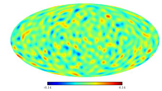
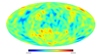
Figure 1: Top: Realization of CIP reconstruction noise assuming a Gaussian CMB temperature field. Bottom: target CIP signal with $A=30$ which is nearly scale-invariant shown with a factor of 10 smaller range than the nearly white noise. Maps have been low pass filtered to $l\leq 30$ to highlight modes where in the curvaton scenario, the temperature-CIP cross correlation can be used to detect the signal.

III.1 CIP Reconstruction

To test the reconstruction pipeline, we begin with the case for which the CIP quadratic estimator was designed Grin et al. (2011b), an otherwise Gaussian random CMB temperature field. In fact, we take the amplitude of the CIP signal to zero to simulate the noise properties of the estimator and in this case the CMB temperature field is completely Gaussian by construction.

Using HEALPix, we draw $n_{\rm sim}=4000$ Gaussian random realizations of the dimensionless temperature fluctuation field $\hat{T}_{lm}$ from the CMB temperature spectrum $C_{l}^{TT}$. Note that this is the power spectrum of the lensed CMB but here the $\hat{T}_{lm}$ do not contain the non-Gaussian correlations of the properly lensed CMB sky. We do this so that we can isolate the non-Gaussian aspects of lensing below. We take $N_{\rm side}=2048$ and $l_{\rm max}=3900$; we have verified that these values yield sufficient accuracy to use modes out to $l=2500$ in the estimator.

From each realization we construct the inverse variance and derivatively filtered fields

$$\hat{T}_{V}(\hat{\bm{n}}) = \sum_{l=2}^{2500}\sum_{m=-l}^{l}\frac{1}{C_{l}^{\tilde{T}\tilde{T}}}\hat{T}_{lm}Y_{lm}(\hat{\bm{n}}),$$

$$\hat{T}_{D}(\hat{\bm{n}}) = \sum_{l=2}^{2500}\sum_{m=-l}^{l}\frac{C_{l}^{\tilde{T},d\tilde{T}}}{C_{l}^{\tilde{T}\tilde{T}}}\hat{T}_{lm}Y_{lm}(\hat{\bm{n}}),$$ (9)

where $C_{l}^{\tilde{T}\tilde{T}}$ is the power spectrum of the unlensed CMB. These filtered fields are then combined to form the minimum variance quadratic estimator for cosmic-variance limited temperature measurements out to $l=2500$ Grin et al. (2011b, 2014)

$$\hat{\Delta}_{LM}=M_{L}\int d\hat{\bm{n}}Y_{LM}^{*}(\hat{\bm{n}}){\hat{T}}_{V}(\hat{\bm{n}}){\hat{T}}_{D}(\hat{\bm{n}}).$$ (10)

Here the normalization

$$\frac{1}{M_{L}} =\sum_{l,l^{\prime}=2}^{2500}\frac{(2l+1)(2l^{\prime}+1)}{4\pi}\left(\begin{array}[]{ccc}l&L&l^{\prime}\\ 0&0&0\\ \end{array}\right)^{2}$$ (13)

$$\quad\times\frac{\big{[}C^{\tilde{T},d\tilde{T}}_{l^{\prime}}+C^{\tilde{T},d\tilde{T}}_{l}\big{]}^{2}}{2C_{l}^{\tilde{T}\tilde{T}}C_{l^{\prime}}^{\tilde{T}\tilde{T}}}$$ (14)

would return an unbiased estimator of the CIP field in the separate universe approximation and in the absence of lensing. Specifically, given that our realizations lack a true CIP signal, the average over the ensemble of temperature realizations

$$\langle\hat{\Delta}_{LM}\rangle=0.$$ (15)

In Fig. 1, we show a single realization of the zero mean noise in the estimator. The noise of the estimator is nearly white. For reference we compare it to a realization of a true CIP signal with $A=30$ which is nearly scale-invariant and hence has relatively more power on large scales. We have also tested this estimator against CMB temperature maps with a true CIP signal following the procedure of Ref. Grin et al. (2014) and find that the reconstruction is unbiased in the absence of lensing-induced off-diagonal correlations.

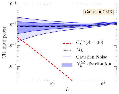
Figure 2: CIP estimator noise power $\hat{N}_{L}^{\Delta\Delta}$ assuming Gaussian CMB maps. Shown are the mean, 68% and 95% confidence bands (shaded) of 4000 realizations of the estimator in the absence of a CIP signal. The mean matches closely the theoretical expectation $M_{L}$ (dotted line) from Eq. (14). The confidence bands match the $\chi^{2}$ expectation of Gaussian noise given the mean (solid lines). For reference we show a true CIP signal with $A=30$ (dashed line).

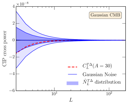
Figure 3: CIP noise cross power $\hat{N}_{L}^{T\Delta}$ assuming Gaussian CMB maps. Shown are the mean, 68% and 95% confidence bands (shaded) of 4000 realizations of the estimator in the absence of a CIP signal. The mean matches closely the theoretical expectation $N_{L}^{T\Delta}=0$ (dotted line). The confidence bands match the Wishart expectation of Gaussian noise (solid lines, see text). For reference we show a true correlated CIP signal with $A=30$ (dashed line).

.

From each realization we construct the all-sky estimator of the auto and cross power spectra of the CIP noise

$$\hat{N}_{L}^{XY}=\frac{1}{2L+1}\sum_{M}\hat{X}_{LM}^{*}\hat{Y}_{LM},$$ (16)

for $X,Y\in T,\Delta$. Averaging the estimators over the ensemble of realizations yields the noise power spectra

$$N_{L}^{XY}=\langle\hat{N}_{L}^{XY}\rangle.$$ (17)

We compare these simulated spectra to the theoretical expectation $N_{L}^{\Delta\Delta}=M_{L}$ and $N_{L}^{T\Delta}=0$ in Figs. 2 and 3 and find good agreement. Given the quadratic nature of the $\Delta$ estimator, $N_{L}^{T\Delta}$ is proportional to the temperature bispectrum which vanishes for a Gaussian temperature field. Note that this agreement also tests the slight mismatch in normalization versus noise due to the use of $C_{l}^{TT}$ for the realizations whereas the filters are built out of the unlensed $C_{l}^{\tilde{T}\tilde{T}}$. We have also tested that $N_{L}^{TT}=C_{L}^{TT}$ as expected.

Using the distribution of realizations $\hat{N}_{L}^{XY}$ we can also test the approximation that the cosmic variance of the quadratic combinations of the temperature field produces nearly Gaussian random noise in the CIP estimator. While the product of Gaussian variates is not Gaussian distributed, the estimator is formed out of many combinations of temperature multipoles. The central limit theorem implies that the noise in the estimator should be much closer to Gaussian than the product of any individual pair.

If the noise in the CIP estimator and the CMB temperature field are themselves Gaussian distributed, the power spectra estimators $\hat{N}_{L}^{XY}$ should be distributed according to a rank 2 Wishart distribution of $2L+1$ degrees of freedom

$$P(\hat{\bf N}_{L}|{\bf N}_{L})=W_{2}\left(\frac{{\bf N}_{L}}{2L+1},2L+1\right).$$ (18)

The Wishart distribution gives the joint probability density of the set of power spectra $\hat{N}_{L}^{XY}$ given $N_{L}^{XY}$ which form $2\times 2$ symmetric matrices $\hat{\bf N}_{L}$ and ${\bf N}_{L}$ with elements $X,Y\in\{T,\Delta\}$. To obtain the marginal probability distribution for a single spectrum e.g. $\hat{N}_{L}^{T\Delta}$ one integrates the joint distribution over the other spectra (see e.g. Ref. Percival and Brown (2006)). The Wishart scale matrix ${\bf N}_{L}/(2L+1)$ reflects the fact that $\hat{\bf N}_{L}$ is defined as the average over the $2L+1$ $M$-modes of the products of the Gaussian fields rather than the sum. For example, rescaling the statistic

$$\frac{2L+1}{N_{L}^{XX}}\hat{N}_{L}^{XX}=\sum_{M=-L}^{L}\frac{\hat{X}_{LM}^{*}\hat{X}_{LM}}{N_{L}^{XX}}$$ (19)

brings its marginal distribution to a $\chi^{2}$ of $2L+1$ degrees of freedom.

In Figs. 2 and 3, we compare the $68\%$ and $95\%$ confidence regions of the $\hat{N}_{L}^{\Delta\Delta}$ and $\hat{N}_{L}^{T\Delta}$ distributions to the Gaussian expectations of the marginal distributions described above. Again we find good agreement, indicating that the noise of the CIP estimator built from quadratic combinations of a Gaussian CMB temperature field is itself nearly Gaussian.

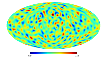
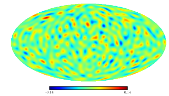
Figure 4: Top: Realization of CIP reconstruction noise using a lensed CMB temperature field. The noise is significantly larger than the Gaussian CMB case of Fig. 1. Bottom: CIP reconstruction averaged over 40 realizations of the CMB sky at recombination lensed by the same potential. CIP reconstruction is biased by the statistical anisotropy of lensing contributing noise that is comparable in amplitude and spectrum to the Gaussian case.

III.2 Lensing Noise

Next we test the reconstruction pipeline with the properly lensed and hence non-Gaussian CMB. In this case we instead draw $4000$ Gaussian random realizations $\tilde{T}_{lm}$ from the unlensed CMB power spectrum $C_{l}^{\tilde{T}\tilde{T}}$ and 4000 lensing potentials $\phi_{lm}$ from $C_{l}^{\phi\phi}$ with correlations consistent with the $C_{l}^{\tilde{T}\phi}$ ISW-lensing cross power Smith and Zaldarriaga (2011); Lewis et al. (2011); Kim et al. (2013); Ade et al. (2015c) as supplied by CAMB.

The angular positions of pixels in the unlensed map are then remapped into the lensed map according to the gradient of the lensing potential Zaldarriaga and Seljak (1999); Hu (2001); Okamoto and Hu (2003)

$$\hat{T}(\hat{\bm{n}})=\tilde{T}(\hat{\bm{n}}+\nabla\phi)$$ (20)

using LensPix. As in the separate universe approximation for CIPs, a large scale lens acts like a position dependent modulation of the CMB and so produces similar effects, in particular an off-diagonal two-point correlation of multipoles moments which biases CIP reconstruction.

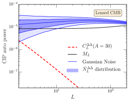
Figure 5: CIP estimator noise power $\hat{N}_{L}^{\Delta\Delta}$ using lensed CMB maps. Shown are the mean, 68% and 95% confidence bands (shaded) of 4000 realizations of the estimator in the absence of a CIP signal. The mean shows an excess of nearly a factor of two from the Gaussian CMB expectation $M_{L}$ (dotted line) from Eq. (14). The confidence bands still match the $\chi^{2}$ expectation of Gaussian noise with this enhanced mean (solid lines). For reference we show a true CIP signal with $A=30$ (dashed line).

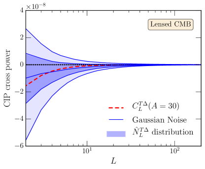
Figure 6: CIP noise cross power $\hat{N}_{L}^{T\Delta}$ using lensed CMB maps. Shown are the mean, 68% and 95% confidence bands (shaded) of 4000 realizations of the estimator in the absence of a CIP signal. The mean carries a nonzero contamination due to the lensing-ISW bispectrum Smith and Zaldarriaga (2011); Lewis et al. (2011); Kim et al. (2013); Ade et al. (2015c) with the Gaussian expectation of zero shown for reference (dotted line). The confidence bands still match the Wishart expectation of Gaussian noise given the mean power spectra (solid lines). For reference we show a true correlated CIP signal with $A=30$ which has a similar spectrum to the contamination (dashed line).

For each realization, we repeat the steps in Eq. (9), (10), (16) and (17) but with these properly lensed temperature maps. In Fig. 4 (top) we show an example realization of the noise in the CIP estimator. In comparison to Fig. 1, the noise is notably larger even though the CMB temperature field that it is constructed from has the same power spectrum $C_{l}^{TT}$ by construction.

This additional noise contribution is from the non-Gaussianity of the lensed CMB. In fact, if the CIP estimator is averaged over the cosmic variance of the CMB at recombination with a fixed realization of the lensing potential $\phi$, lensing produces a bias in the CIP map itself

$$\langle\hat{\Delta}_{LM}\rangle\big{|}_{\phi}\neq 0,$$ (21)

due to the statistical anisotropy that it creates. In Fig. 4 (bottom), we separately perform such an average over 40 unlensed $\tilde{T}_{lm}$ CMB realizations lensed by the same potential. Notice that the fake CIP signal induced by the fixed $\phi$ has roughly the same amplitude and spectrum as the Gaussian CMB contribution to the CIP noise in Fig. 1 (top).

Of course once averaged over random realization of the lens potential as in our main $n_{\rm sim}$ realizations, the bias due to the statistical anisotropy of the lens becomes a non-Gaussian CMB source of zero mean noise. In Fig. 5, we show that the non-Gaussian lensing contribution nearly doubles the noise power in $N_{L}^{\Delta\Delta}$. Furthermore, the lensing-ISW correlation Smith and Zaldarriaga (2011); Lewis et al. (2011); Kim et al. (2013); Ade et al. (2015c) produces a nonzero $N_{L}^{T\Delta}$ as well (see Fig. 6). This fake CIP-temperature correlation has a spectrum that is similar but not identical to that predicted by the curvaton model and so error propagation in its removal is important to model.

In spite of their origin in the non-Gaussianity of the lensed CMB, these excess contributions to the noise in the CIP estimator are nearly Gaussian distributed. In Fig. 5 and 6, we compare the distributions of $\hat{N}_{L}^{\Delta\Delta}$ and $\hat{N}_{L}^{T\Delta}$ to the Gaussian noise expectation. Even the tails of the distribution as displayed by the 95% confidence region are well modeled by a multivariate Gaussian.

For the CIP estimator noise to be Gaussian random, the covariance of the noise power must be diagonal in $L$, not just Wishart distributed in its variance.To test this, we construct the covariance matrix of $\hat{N}_{L}^{\Delta\Delta}$:

$$C_{ij}\equiv\langle\hat{N}_{L_{i}}^{\Delta\Delta}\hat{N}_{L_{j}}^{\Delta\Delta}\rangle-N_{L_{i}}^{\Delta\Delta}N_{L_{j}}^{\Delta\Delta}.$$ (22)

In Fig. 7, we show the correlation matrix

$$R_{ij}=\frac{C_{ij}}{\sqrt{C_{ii}C_{jj}}}.$$ (23)

The off-diagonal $i\neq j$ elements are consistent with zero up to the expected $n_{\rm sim}^{-1/2}$ statistical fluctuations due to the finite sample.

To quantify these bounds, we calculate the mean of the off-diagonal correlations

$$R=\frac{2}{n_{L}(n_{L}-1)}\sum_{i,j>i}R_{ij},$$ (24)

where $n_{L}$ is the number of multipoles $L\in[2,200]$, and find a negligible $R=0.00053$ and the variance

$$\sigma_{R}^{2}=\frac{2}{n_{L}(n_{L}-1)}\sum_{i,j>i}R_{ij}^{2}-R^{2}$$ (25)

which gives $\sigma_{R}=0.016$. In Fig. 8, we further test that the scaling of $\sigma_{R}$ with $n_{\rm sim}$ by using the first $n_{\rm sim}$ of the full 4000 set shows no sign of a deviation from $n_{\rm sim}^{-1/2}$ that would indicate an underlying correlation.

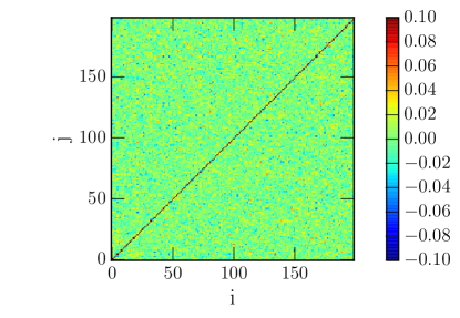
Figure 7: Correlation matrix $R_{ij}$ between multipoles $L_{i}$ and $L_{j}$ of the CIP noise power $\hat{N}_{L}^{\Delta\Delta}$ (Eq. 23) using 4000 realizations of the lensed CMB maps. The diagonal is removed to display the off-diagonal terms which fluctuate around a mean of $R=0.00053$ with an r.m.s. $\sigma_{R}=0.016$ as consistent with the finite number of realizations.

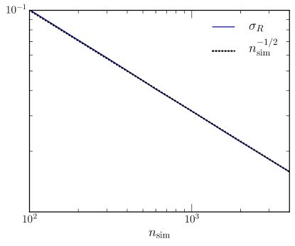
Figure 8: The r.m.s fluctuations in the off-diagonal correlations $\sigma_{R}$ vs. the number of simulations $n_{\mathrm{sim}}$ for multipoles $L\in[2,200]$. The dispersion $\sigma_{R}$ (solid) scales as $n_{\mathrm{sim}}^{-1/2}$ (dotted), as expected for statistical fluctuations around an insignificant correlation.

Finally we test that binning the multipoles decreases the variance in the noise power in the manner expected for independent Gaussian random variables. The statistic

$$\nu\hat{V}_{L_{1},L_{2}}\equiv\sum_{L=L_{1}}^{L_{2}}(2L+1)\frac{\hat{N}_{L}^{\Delta\Delta}}{N_{L}^{\Delta\Delta}}$$ (26)

should be distributed as a $\chi^{2}$ with $\nu$ degrees of freedom (see Eq. 19) where

$$\nu=\sum_{L=L_{1}}^{L_{2}}(2L+1)=(L_{2}+1)^{2}-L_{1}^{2}.$$ (27)

In Fig. 9, we show that the distribution of $\hat{V}_{31,40}$ in the 4000 simulations is in good agreement with the $\chi^{2}$ distribution. Other bins show the same level of agreement, which directly tests the approach taken in the next section of combining the information from each multipole as if they were independent.

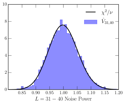
Figure 9: Binned and normalized noise power $\hat{V}_{31,40}$ distribution for the multipole band $L=31-40$. The distribution is well modeled by the Gaussian noise expectation that $\nu\hat{V}_{31,40}$ is distributed as a $\chi^{2}$ with $\nu=720$ degrees of freedom.

Table 1: $2\sigma_{A}$ detection threshold for $A$ given various noise assumptions for CIPs that are correlated with CMB temperature fluctuations and uncorrelated. Here CIPs are reconstructed to multipole $L_{\rm CIP}=100$ from quadratic estimators with cosmic-variance limited CMB temperature measurements out to $l=2500$.

	$2\sigma_{A}$
Noise	Corr. CIP	Uncorr. CIP
Gaussian CMB Analytic	24	45
Gaussian CMB Sim.	25	47
Lensed CMB Sim.	31	58

IV Forecasts

In the previous section we have shown that the non-Gaussianity of the lensed CMB nearly doubles the noise power of the CIP estimator for cosmic-variance limited temperature measurements out to $l=2500$. This has a substantial impact on the detectability of CIPs that we address in this section.

Even when the significant non-Gaussian effects of lensing are included, the total noise in the CIP estimator is nearly Gaussian distributed (see Sec. III.2). This means that we can treat the total noise like detector noise or cosmic variance in the data analysis. To estimate the impact of the lensing contributions on the detection of the CIP amplitude $A$, we use the Fisher matrix. We focus on CIP reconstruction using cosmic-variance limited measurements of the CMB temperature field out to $l=2500$ as in the simulations of the previous section. We also simplify the analysis by assuming that all cosmological parameters except for $A$ are fixed.

Under these assumptions the Fisher matrix has a single entry whose inverse is the estimate of the variance of measurements of $A$, $\sigma_{A}^{2}$. It combines the information from the various CIP power spectra and multipole moments

$$\sigma_{A}^{-2}=\sum_{L=2}^{L_{\rm CIP}}\sum_{XY,X^{\prime}Y^{\prime}}\frac{\partial C_{L}^{XY}}{\partial A}\left({\bf C}^{-1}_{L}\right)_{XY,X^{\prime}Y^{\prime}}\frac{\partial C_{L}^{X^{\prime}Y^{\prime}}}{\partial A},$$ (28)

where as before $X,Y\in\{T,\Delta\}$ and ${\bf C}_{L}$ is the covariance matrix

$${\bf C}^{XY,X^{\prime}Y^{\prime}}_{L}=\frac{{\tilde{C}_{L}^{XX^{\prime}}\tilde{C}_{L}^{YY^{\prime}}+\tilde{C}_{L}^{XY^{\prime}}\tilde{C}_{L}^{X^{\prime}Y}}}{2L+1}.$$ (29)

We only include $L<L_{\rm CIP}=100$ in order to remain in the regime where the separate-universe assumption made in constructing the estimator is valid He et al. (2015).

The difference between this covariance and that implied by the Wishart distribution of the previous section is that we now include the sample variance of a real CIP signal

$$\tilde{C}_{L}^{\Delta\Delta} = C_{L}^{\Delta\Delta}+N_{L}^{\Delta\Delta},$$

$$\tilde{C}_{L}^{T\Delta} = C_{L}^{T\Delta}+N_{L}^{T\Delta},$$

$$\tilde{C}_{L}^{TT} = C_{L}^{TT}=N_{L}^{TT}.$$ (30)

The sample variance depends on the assumed value of $A$ and so we take its value to be the detection threshold $A=2\sigma_{A}$ for the various simulated and analytic noise spectra $N_{L}^{XY}$ from the previous section (see Tab. 1).

To establish the baseline, we start with the analytic form for the noise given a Gaussian CMB in the absence of CIPs and lensing as in Ref. He et al. (2015),

$$N_{L}^{\Delta\Delta} = M_{L},\quad N_{L}^{T\Delta}=0,$$ (31)

for which 2$\sigma_{A}=24$ with correlated CIPs. Employing instead the Gaussian CMB simulations for the noise spectra we obtain a consistent $2\sigma_{A}=25$. Finally with the lensed CMB simulations the threshold is raised to $2\sigma_{A}=31$, a factor of $\sim$1.3 higher compared to the case of analytical estimate of the noise for Gaussian CMB.

Given that these detection thresholds are larger than even the largest curvaton motivated value, it is also interesting to consider the case of uncorrelated CIPs $C_{L}^{T\Delta}=0$ with the same $C_{L}^{\Delta\Delta}$. We find that the lensing noise contributes here as well by raising the $2\sigma$ threshold a factor of $\sim 1.3$ from 45 to 58.

If we take $L_{\rm CIP}=200$, the detection thresholds are slightly lower in the correlated case but the relative degradation from lensing is similar. In the uncorrelated case, the results are insensitive to the exact value of $L_{\rm CIP}$ since most of the signal-to-noise comes from large scales for a nearly scale invariant auto-spectrum.

V Conclusions

A large scale CIP field modulates the two point statistics of small scale CMB anisotropies, much like gravitational lensing. The quadratic reconstruction of the former from the latter can therefore be contaminated by lensing. We have shown, using simulations, that non-Gaussian modulation by lensing provides an additional contribution to the noise in the CIP estimator that is comparable to that of the cosmic variance of the small scale CMB modes themselves. Moreover, the lensing-ISW bispectrum (present in the absence of real CIPs) Goldberg and Spergel (1999); Smith and Zaldarriaga (2011); Lewis et al. (2011); Kim et al. (2013); Ade et al. (2015c) provides a false signal that resembles the CIP-temperature cross correlation in the curvaton model; such contamination similarly afflicts estimators of the amplitude $f_{\rm NL}$ of primordial local-type non-Gaussianity Goldberg and Spergel (1999); Smith and Zaldarriaga (2011); Lewis et al. (2011); Kim et al. (2013); Ade et al. (2015b).

Despite these non-Gaussian effects in the CMB, the resultant noise in the CIP estimator is nearly Gaussian by virtue of the central limit theorem. We find that the noise power is uncorrelated to good approximation – no more than 0.1% correlations averaged over all multipole pairs with pair fluctuations that are consistent with our finite sample of simulations and less than $2\%$. Furthermore, binning of multipoles reduces the variance of the noise power in the same manner as a Gaussian random field.

Treating the lensing contamination as excess Gaussian random noise, we estimate its impact on the detection of CIPs using the Fisher information matrix. Assuming cosmic-variance limited measurements of the CMB temperature anisotropies out to $l=2500$, we find that the detection thresholds for the CIP amplitude parameter $A$ are raised by a factor of 1.3 when the lensing bias is included for both the uncorrelated and correlated CIPs. Here we have employed CIP reconstruction up to the separate-universe limit $L_{\rm CIP}=100$ and assumed all other cosmological parameters are fixed.

Our methodology, which employs direct simulation of lensing, is also straightforward to generalize to cases where measurement noise, systematic effects and other cosmological parameters are included. In these cases the lensing contamination is treated as an additional signal that is jointly modeled along with the CIP contributions and prior information in a realistic data pipeline. Cosmological parameter uncertainties can make the lensing contamination even more important given parameter degeneracies. For example the ISW-lensing contamination Smith and Zaldarriaga (2011); Lewis et al. (2011); Kim et al. (2013); Ade et al. (2015c), depends on the cosmic acceleration model and takes a similar form to the CIP cross correlation. Fortunately, the lensing contamination to the CIP auto correlation takes a very different form which can be used to break degeneracies.

Likewise, CMB polarization information can also assist in distinguishing lensing from CIPs as well as reduce the overall noise in the CIP estimator. In particular quadratic reconstruction from the $E$ and $B$ modes has the highest signal-to-noise for lensing reconstruction Hu and Okamoto (2002) and the lowest for CIP reconstruction He et al. (2015). More generally, these additional fields provide consistency tests for the specific type of modulation expected by CIPs in the auto and cross power spectra of their quadratic estimators.

Finally, there are consistency tests that are internal to just the temperature based CIP estimator. The estimator is constructed out of many pairs of temperature multipoles whose weights were chosen to be optimal in the absence of lensing. Whereas the impact of CIP modulation does not depend strongly on the orientation of the modes, lensing does since its effect vanishes if the deflection is in a direction orthogonal to the modes. In principle, the pairs can be reweighted to de-emphasize the most contaminated modes at the expense of computational efficiency of the estimator. We leave these topics for future study.