Supporting the search for the CEP location with nonlocal PNJL models constrained by Lattice QCD

Abstract

We investigate the possible location of the critical endpoint in the QCD phase diagram based on nonlocal covariant PNJL models including a vector interaction channel. The form factors of the covariant interaction are constrained by lattice QCD data for the quark propagator. The comparison of our results for the pressure including the pion contribution and the scaled pressure shift $\Delta P/T^{4}$ vs $T/T_{c}$ with lattice QCD results shows a better agreement when Lorentzian formfactors for the nonlocal interactions and the wave function renormalization are considered. The strength of the vector coupling is used as a free parameter which influences results at finite baryochemical potential. It is used to adjust the slope of the pseudocritical temperature of the chiral phase transition at low baryochemical potential and the scaled pressure shift accessible in lattice QCD simulations. Our study, albeit presently performed at the meanfield level, supports the very existence of a critical point and favors its location within a region that is accessible in experiments at the NICA accelerator complex.

The search for the location of the critical endpoint (CEP) of first order phase transitions in the QCD phase diagram is one of the objectives for beam energy scan (BES) programs in relativistic heavy-ion collision experiments at RHIC and SPS as well as in future ones at NICA and FAIR which try to identify the parameters of its position $(T_{\rm CEP}$, $\mu_{\rm CEP})$. From a theoretical point of view, the situation is very blurry since the predictions for this position form merely a skymap in the $T$-$\mu$ plane Stephanov:2007fk .

Lattice QCD results at zero and small chemical potential $\mu$, show that the chiral and deconfinement transitions are crossover with a pseudocritical temperature of $T_{c}(0)=154\pm 9$ MeV Bazavov:2011nk .

However, at finite density lattice QCD suffers from the sign problem and only extrapolation or approximate techniques are available that work at finite quark densities. Therefore, nonperturbative methods and effective models are inevitable tools in this region. Up to now, such effective low-energy QCD approaches are not yet sufficiently developed to provide a unified approach to quark-hadron matter where hadrons appear as strongly correlated (bound) quark states that eventually dissolve into their quark (and gluon) constituents in the transition from the hadronic phase with confined quarks to the quark gluon plasma. Since this transition shall be triggered by chiral symmetry restoration (by lowering the thresholds for hadron dissociation determined by in-medium quark masses), we expect that a first step towards a theoretical approach to the QCD phase diagram is the determination of order parameters characterizing the QCD phases in a meanfield approximation for chiral quark models of different degree of sophistication. As a consequence there appeared a variety of possibilities for the structure of the QCD phase diagram and the position of the CEP in the literature. Let us mention few of them:

• no CEP at all Bratovic:2012qs , with crossover transition in the whole phase diagram,

• no CEP, but a Lifshitz point Carignano:2010 ,

• one CEP, but with largely differing predictions of its position Stephanov:2007fk ,

• second CEP Kitazawa:2002bc ; Blaschke:2003cv ; Hatsuda:2006ps ,

• CEP and triple point, possibly coincident, considering another phase (i.e. color superconducting Blaschke:2004cc or quarkyonic Andronic:2009gj matter) at low temperatures and high densities.

This situation is far from being satisfactory in view of the upcoming experimental programmes. An exhaustive analysis should be performed to predict a CEP region as narrow as possible, considering only those effective models that best reproduce recent lattice QCD results on the one hand and that obey constraints from heavy-ion collision experiments and compact star observations where available.

In the present contribution, we discuss the existence and location of a CEP within the class of nonlocal chiral quark models coupled to the Polyakov loop (PL) potential, with vector channel interactions, on the selfconsistent meanfield level, contrasting our results with those of the widely used local PNJL models that appear as limiting case of the present approach.

The Lagrangian of these models is given by

$${\mathcal{L}}=\bar{q}(i\not{D}-m_{0})q+{\mathcal{L}}_{\rm int}+{\cal{U}}(\Phi)~{},$$ (1)

where $q$ is the $N_{f}=2$ fermion doublet $q\equiv(u,d)^{T}$, and $m_{0}$ is the current quark mass (we consider isospin symmetry, that is $m_{0}=m_{u}=m_{d}$). The covariant derivative is defined as $D_{\mu}\equiv\partial_{\mu}-iA_{\mu}$, where $A_{\mu}$ are color gauge fields.

The nonlocal interaction channels are given in the current-current coupling form by

$${\mathcal{L}}_{\rm int}=-\frac{G_{S}}{2}\Big{[}j_{a}(x)j_{a}(x)-j_{P}(x)j_{P}(x)\Big{]}{-}\frac{G_{V}}{2}j_{V}(x)\,j_{V}(x),$$

where the nonlocal generalizations of the currents are

$$j_{a}(x) = \int d^{4}z\ g(z)\ \bar{q}\left(x+\frac{z}{2}\right)\ \Gamma_{a}\ q\left(x-\frac{z}{2}\right)\ ,$$

$$j_{P}(x) = \int d^{4}z\ f(z)\ \bar{q}\left(x+\frac{z}{2}\right)\ \frac{i{\overleftrightarrow{\hbox to0.0pt{/\hss}\partial}}}{2\ \kappa_{p}}\ q\left(x-\frac{z}{2}\right)\ ,$$

$$j_{V}(x) = \int d^{4}z\ g(z)\ \bar{q}\left(x+\frac{z}{2}\right)\,\gamma^{0}\ q\left(x-\frac{z}{2}\right).$$ (3)

with $\Gamma_{a}=(\Gamma_{S},\Gamma_{P})=(\leavevmode\hbox{\small 1\kern-3.8pt\normalsize 1},i\gamma_{5}\vec{\tau})$ for scalar and pseudoscalar currents respectively, and $u(x^{\prime}){\overleftrightarrow{\partial}}v(x)=u(x^{\prime})\partial_{x}v(x)-\partial_{x^{\prime}}u(x^{\prime})v(x)$. The functions $g(z)$ and $f(z)$ in Eq. (3) are nonlocal covariant form factors characterizing the corresponding interactions. The scalar-isoscalar component of the $j_{a}(x)$ current will generate the momentum dependent quark mass in the quark propagator, while the “momentum” current, $j_{P}(x),$ will be responsible for a momentum dependent wave function renormalization (WFR) of this propagator. Note that the relative strength between both interaction terms is controlled by the mass parameter $\kappa_{p}$ introduced in Eq. (3). Finally, $j_{V}(x)$ represents the vector channel interaction current, whose coupling constant $G_{V}$ is usually taken as a free parameter.

In what follows it is convenient to Fourier transform into momentum space. Since we are interested in studying the characteristics of the chiral phase transition we have to extend the effective action to finite temperature $T$ and chemical potential $\mu$. In the present work this is done by using the Matsubara imaginary time formalism. Concerning the gluon degrees of freedom we employ the PL extension of nonlocal chiral quark models according to previous works Contrera:2007wu ; Contrera:2010kz ; Horvatic:2010md ; Radzhabov:2010dd ; Benic:2013eqa , i.e. assuming that the quarks move in a background color gauge field $\phi=iA_{0}=ig\,\delta_{\mu 0}\,G^{\mu}_{a}\lambda^{a}/2$, where $G^{\mu}_{a}$ are the SU(3) color gauge fields and $\lambda^{a}$ are the Gell-Mann matrices. Then the traced PL $\Phi$, which is taken as order parameter of confinement, is given by $\Phi=\frac{1}{3}{\rm Tr}\,\exp(i\phi/T)$. Then, working in the so-called Polyakov gauge, in which the matrix $\phi$ is given by a diagonal representation $\phi=\phi_{3}\lambda_{3}+\phi_{8}\lambda_{8}$. At vanishing chemical potential, owing to the charge conjugation properties of the QCD Lagrangian, the traced PL is expected to be a real quantity. Since $\phi_{3}$ and $\phi_{8}$ have to be real-valued Rossner:2007ik , this condition implies $\phi_{8}=0$. In general, this need not be the case at finite $\mu$ Dumitru:2005ng ; Fukushima:2006uv . As, e.g., in Refs. Contrera:2010kz ; Rossner:2007ik ; Abuki:2008ht ; GomezDumm:2008sk we will assume that the potential $\cal U$ is such that the condition $\phi_{8}=0$ is well satisfied for the range of values of $\mu$ and $T$ investigated here. The mean field traced PL is then given by

$$\Phi=\frac{1}{3}\Big{[}1+2\,\cos(\phi_{3}/T)\Big{]}.$$ (4)

In the present work we have chosen a $\mu$-dependent logarithmic effective potential described in Dexheimer:2009va .

$${\cal{U}}(\Phi,T,\mu)= (a_{0}T^{4}+a_{1}\mu^{4}+a_{2}T^{2}\mu^{2})\Phi^{2}$$ (5)

$$+a_{3}T_{0}^{4}\ln{(1-6\Phi^{2}+8\Phi^{3}-3\Phi^{4})},$$

where the parameters are $a_{0}=-1.85$, $a_{1}=-1.44$x$10^{-3}$, $a_{2}=-0.08$, $a_{3}=-0.40$. For the $T_{0}$ parameter we use the value corresponding to two flavors $T_{0}=208$ MeV, as has been suggested in Ref. Schaefer:2007pw and already employed in nonlocal PNJL models in Horvatic:2010md ; Pagura:2012 .

Finally, in order to fully specify the nonlocal model under consideration we set the model parameters as well as the form factors $g(q)$ and $f(q)$ following Refs. Contrera:2010kz , Noguera:2008prd78 and Contrera:2012wj , i.e. considering two different types of functional dependencies for these form factors: exponential forms

$$(\textrm{Set A})\quad\left\{\begin{array}[]{l}g(p)=\mbox{exp}\left(-p^{2}/\Lambda_{0}^{2}\right)\\ f(p)=0\end{array}\right.~{},$$ (8)

$$(\textrm{Set B})\quad\left\{\begin{array}[]{l}g(p)=\mbox{exp}\left(-p^{2}/\Lambda_{0}^{2}\right)\\ f(p)=\mbox{exp}\left(-p^{2}/\Lambda_{1}^{2}\right)\end{array}\right.~{},$$ (11)

and Lorentzians with WFR

$$(\textrm{Set C})\quad\left\{\begin{array}[]{l}g(p)=\frac{1+\alpha_{z}}{1+\alpha_{z}\ f_{z}(p)}\frac{\alpha_{m}\ f_{m}(p)-m\ \alpha_{z}f_{z}(p)}{\alpha_{m}-m\ \alpha_{z}}\\ f(p)=\frac{1+\alpha_{z}}{1+\alpha_{z}\ f_{z}(p)}f_{z}(p)\end{array}\right.~{},$$ (14)

where

$$f_{m}(p)=\left[1+\left(p^{2}/\Lambda_{0}^{2}\right)^{3/2}\right]^{-1},$$

$$f_{z}(p)=\left[1+\left(p^{2}/\Lambda_{1}^{2}\right)\right]^{-5/2},$$ (15)

and $\alpha_{m}=309$ MeV, $\alpha_{z}=-0.3$. Further details on the parameters can be found in Ref. Contrera:2012wj and references quoted therein.

Within this framework the thermodynamic potential in the mean field approximation (MFA) reads

$$\Omega^{\rm MFA}= -\,{4T}\sum_{c}\sum_{n}\int\frac{d^{3}\vec{p}}{(2\pi)^{3}}\,\,\mbox{ln}\left[\frac{(\tilde{\rho}_{n,\vec{p}}^{c})^{2}+M^{2}(\rho_{n,\vec{p}}^{c})}{Z^{2}(\rho_{n,\vec{p}}^{c})}\right]$$ (16)

$$+\frac{\sigma_{1}^{2}+\kappa_{p}^{2}\ \sigma_{2}^{2}}{2\,G_{S}}-\frac{\omega^{2}}{2G_{V}}\ +{\cal{U}}(\Phi,T).$$

where $M(p)$ and $Z(p)$ are given by

$$M(p) = Z(p)\left[m+\sigma_{1}\ g(p)\right],$$

$$Z(p) = \left[1-\sigma_{2}\ f(p)\right]^{-1}.$$ (17)

In addition, we have defined Blaschke:2007ri

$$\Big{(}{\rho_{n,\vec{p}}^{c}}\Big{)}^{2}=\Big{[}(2n+1)\pi T-i\mu+\phi_{c}\Big{]}^{2}+{\vec{p}}\ \!^{2}\ ,$$ (18)

where the quantities $\phi_{c}$ are given by the relation $\phi_{c}={\rm diag}(\phi_{r},\phi_{g},\phi_{b})$. Namely, $\phi_{c}=c\ \phi_{3}$ with $c=1,-1,0$ for $r,g,b$, respectively.

In the case of $\Big{(}{\tilde{\rho}_{n,\vec{p}}^{c}}\Big{)}$ we have used the same definition as in Eq.(18) but shifting the chemical potential according to Contrera:2012wj

$$\tilde{\mu}=\mu\;-\omega\;g(p)\;Z(p).$$ (19)

We also want to include in our analysis the results arising from a local PNJL model based on Fukushima2008 with two flavors instead of three. Moreover, we consider that the chemical potential is shifted by

$$\tilde{\mu}=\mu\;-\omega.$$ (20)

$\Omega^{\rm MFA}$ turns out to be divergent and, thus, needs to be regularized. For this purpose we use the same prescription as in Refs. Dumm:2005 ; Contrera:2010kz . The mean field values $\sigma_{1,2}$, $\omega$ and $\phi_{3}$ at a given temperature or chemical potential, are obtained from a set of four coupled “gap” equations which come from the minimization of the regularized thermodynamic potential, that is

$$\frac{\partial\Omega^{\rm MFA}_{\rm reg}}{\partial\sigma_{1}}=\frac{\partial\Omega^{\rm MFA}_{\rm reg}}{\partial\sigma_{2}}=\frac{\partial\Omega^{\rm MFA}_{\rm reg}}{\partial\omega}=\frac{\partial\Omega^{\rm MFA}_{\rm reg}}{\partial\phi_{3}}=0.$$ (21)

As a starting point we consider the local NJL, using in this case the parameters as in GomezDumm:2008sk . This resembles the local limit of the present model and results can be compared, e.g., with Refs. Bratovic:2012qs and Friesen:2014mha . As in our previous work Contrera:2012wj , the model inputs have been constrained with results from lattice QCD studies. In particular, the form factors of the nonlocal interaction can be chosen such as to reproduce the dynamical mass function $M(p)$ and the WFR function $Z(p)$ of the quark propagator in the vacuum Parappilly:2005ei . In Fig. 1 we show the shapes of normalized dynamical masses and WFR for the models under discussion here, i.e., the nonlocal models of Set A (rank-one), Set B and Set C (rank-two) as well as the local limit. From this figure we see that Set C fits best the normalized dynamical mass.

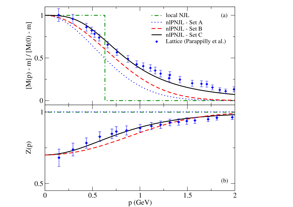
Figure 1: Normalized dynamical masses for the different form factors under study and wave function renormalization for Set B and Set C, fitted to lattice QCD data Parappilly:2005ei . (Adapted from Ref. Noguera:2008prd78 ).

Now we are in the position to discuss the results for the thermodynamics of the nonlocal PNJL models, starting from the pressure $P(\mu,T)=-\Omega^{\rm MFA}_{\rm reg}$. In the upper panel of Fig. 2 we compare the pressure shift $\Delta P=P(\mu,T)-P(0,T)$ scaled with $T^{4}$ as a function of $T/T_{c}$ for all sets of parametrizations shown in Fig. 1 to lattice results from Allton:2003vx ; Fodor:2002km . It is obvious that the best obtained fit corresponds to Set C, supporting the robustness of rank-2 Lorentzian parametrization. In the lower panel of Fig. 2 we show a comparison between Set C and lattice results Allton:2003vx , for $G_{V}=0.0$ (i.e. without vector interactions).

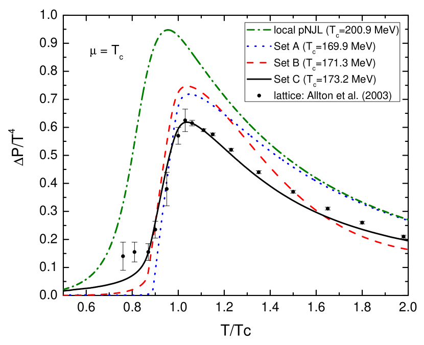
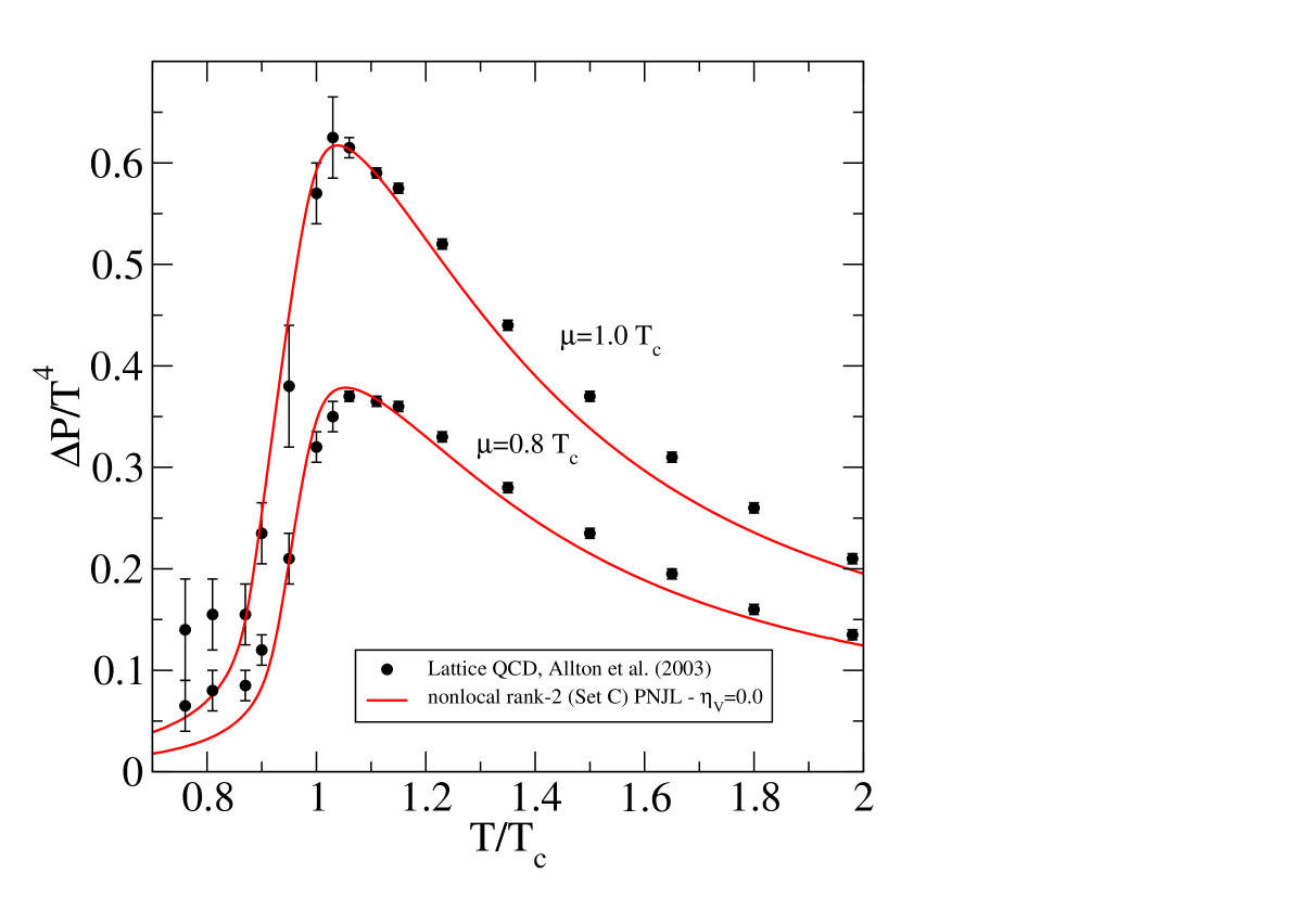
Figure 2: The scaled pressure shift $\Delta P/T^{4}$ as a function of the scaled temperature $T/T_{c}$, for $G_{V}=0.0$. Upper panel: Comparison of the lattice QCD data Allton:2003vx with results of local and nonlocal pNJL models. Lower panel: Comparison of Set C results with lattice QCD Allton:2003vx for two chemical potentials $\mu=1.0~{}T_{c}$ and $\mu=0.8~{}T_{c}$.

In Fig. 3 we show a comparison of the pressure normalized to the Stefan-Boltzmann limit ($P_{\rm SB}$) to lattice QCD results from AliKhan:2001ek . In this figure it can be seen that the pion pressure dominates the pressure dependence for $T<T_{c}$ and quickly vanishes for $T>T_{c}$ as a result of the Mott dissociation of the pion.

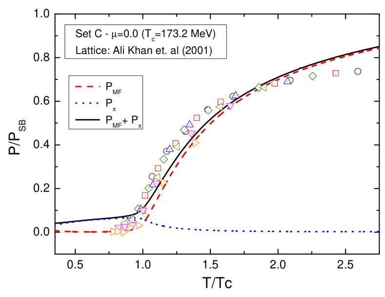
Figure 3: Comparison of the pressure in units of its Stefan-Boltzmann value between Set C (with and without pion pressure) and lattice QCD results AliKhan:2001ek as function of $T/T_{c}$.

From the above results, Set C appears to be the appropriate choice to best fit lattice QCD results.

As mentioned above, the vector coupling $G_{V}$ is considered a free parameter. In Fig. 4 we show again $\Delta P/T^{4}$ vs. $T/T_{c}$ as in Fig. 2, but now considering different vector coupling parameters $\eta_{V}=G_{V}/G_{S}$ just for Set C and $\mu=T_{c}$. The best agreement with lattice QCD data is obtained for $\eta_{V}=0$, i.e. for the deactivated vector channel. The consequences will be discussed below.

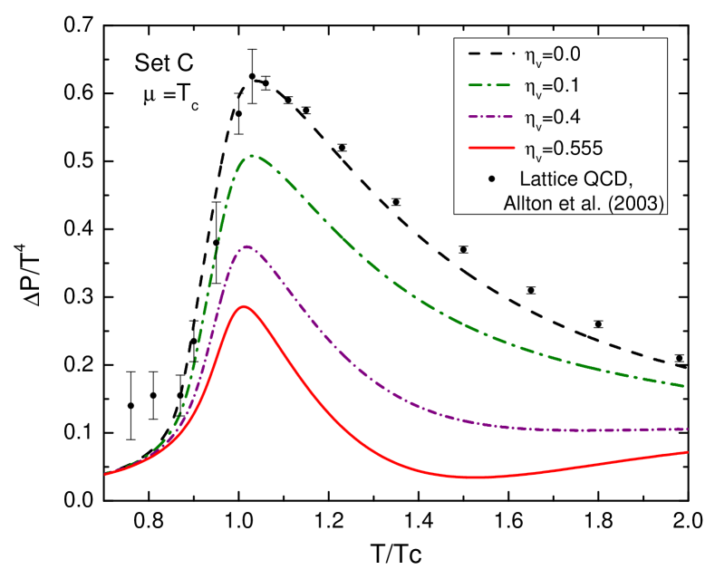
Figure 4: Comparison between Set C results for different values of the vector coupling parameter $\eta_{V}$ and lattice QCD data Allton:2003vx .

In MFA the vector coupling channel has a direct influence on the $\mu-$dependence of the pseudocritical temperature $T_{c}(\mu)$ in the QCD phase diagram. In lattice QCD this dependence has been analyzed by Taylor expansion techniques Kaczmarek:2011zz as

$$T_{c}(\mu)/T_{c}(0)=1-\kappa(\mu/T)^{2}+{\mathcal{O}}[(\mu/T)^{4}],$$ (22)

with $\kappa=0.059(2)(4)$ being the curvature. We will refer to this situation as LR I (lattice results I). In the same way, the vector coupling channel can be tuned to reproduce the curvature given by recent lattice QCD results based on imaginary chemical potential technique which gives $\kappa=0.1341\pm 0.019$ Bellwied:2015rza and $\kappa=0.1215\pm 0.018$ Bonati:2015bha , we call it LR II.

The curvatures can be determined from the phase diagrams. To do so, we plotted the pseudocritical temperatures of the crossover transitions as a function of $(\mu/T)^{2}$ for different values of the vector coupling parameter $\eta_{V}$. Then, the curvatures can be obtained from the slope of the straight lines in the region of low $(\mu/T)$ values.

An example of this is shown in Figure 5 for set C (the corresponding plots for the other sets are qualitatively very similar). The fit (22) of the lattice QCD results, LR I, is also shown. The grey zone corresponds to the error in the coefficient $\kappa$ obtained in Kaczmarek:2011zz .

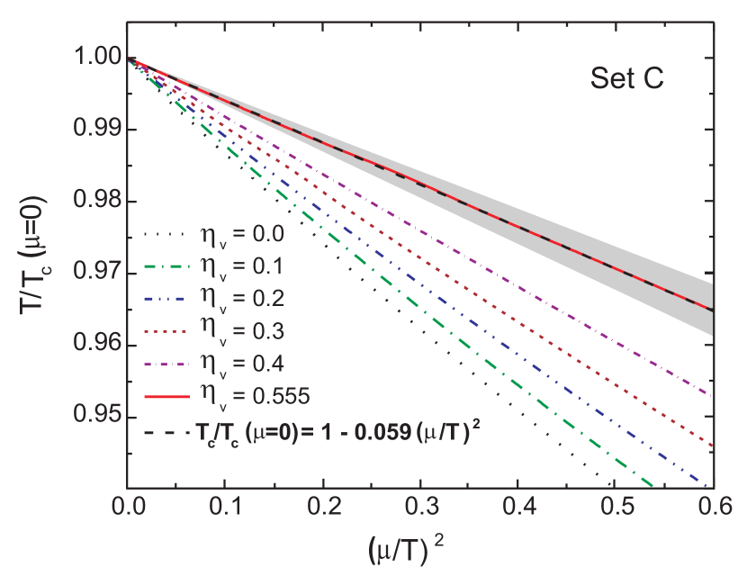
Figure 5: (Color online) Chiral crossover transitions at low values of $\mu/T$ for different values of the vector coupling ratios $\eta_{V}=G_{V}/G_{S}$ for Set C. The dashed line corresponds to the lattice QCD prediction of $\kappa=0.059(2)(4)$, LR I, Kaczmarek:2011zz .

In Fig. 6 we compare the lattice QCD results for both, LR I and LR II, with the values for the coefficient $\kappa$ obtained within all PNJL models under study, considering different values of $\eta_{V}$.

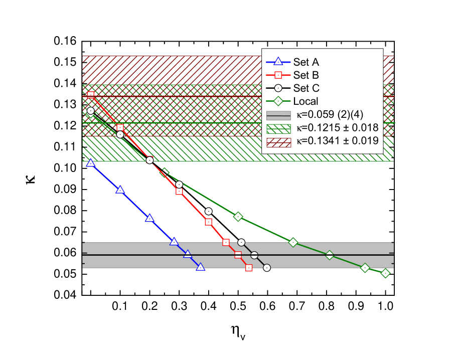
Figure 6: (Color online) Curvature $\kappa$ of the pseudocritical temperature $T_{c}(\mu)$ of the chiral crossover transition at low values of $\mu/T$. The black line corresponds to the lattice QCD prediction of $\kappa=0.059(2)(4)$ Kaczmarek:2011zz , while the brown (green) lines with hatched error regions come from analyses within the imaginary chemical potential method, resulting in $\kappa=0.1341\pm 0.019$ Bellwied:2015rza ($\kappa=0.1215\pm 0.018$ Bonati:2015bha ).

Note that for fitting the lattice QCD value in the local model a larger vector coupling is required than in the nonlocal ones, as is shown in Ref.Contrera:2012wj . Also the absolute value of the critical temperature $T_{c}(0)$ in the local model is significantly different (larger) than in the nonlocal one.

The phase diagram with (pseudo-)critical temperatures $T_{c}(\mu)$ and critical points for Set C, i.e. the parametrization that best fits lattice QCD results (see Figs. 1 to 3) are shown in Fig. 7. The finite vector coupling parameter $\eta_{V}$ is chosen to reproduce the curvature value for LR I at low $\mu$. We found that switching off the vector interaction can reproduce both, the curvature obtained in LR II and the $\Delta P/T^{4}$ vs. $T/T_{c}$ from Fig. 2 .

Now we also considered the pseudo-critical deconfinement lines for $\Phi=0.4-0.6$ in Fig. 7. To determine them we proceed as follows: we set the fixed value of $\Phi$ in Eq. (4), obtaining a relation between $\phi_{3}$ and T. Then we replace this relation in the thermodynamic potential and minimize it respect to the mean fields by solving the Eqs. (21). Thus, for each value of $\Phi$ we have the corresponding values of $\phi_{3}$ and T that satisfy the Eq. (4) and the gaps equations for the desired value of $\Phi$. Those are the deconfinement lines at fixed $\Phi$ shown in Fig. 7. However, this tells us only that the PL changes quickly with $T$, but not how much confining the model is still at high $T$. Since obviously the change occurs at absolute values of $\Phi\leq 0.4$, there are still strong color correlations present in the system at high temperatures.

In order to estimate the region in the phase diagram where we expect color correlations as measured by the value of the Polyakov loop to be strong, we choose to show the lines of constant $\Phi$. Interestingly, we find that in the presence of a vector meanfield the approach to the free quasiparticle case ($\Phi=1$) is inhibited. It is clear that this is the more so the larger the chemical potential is since the vector meanfield is proportional to the baryon density which increases with $\mu$.

On the other hand, the PL transition as defined by the peak of the PL thermal susceptibility coincides nicely with that of the crossover chiral transition.

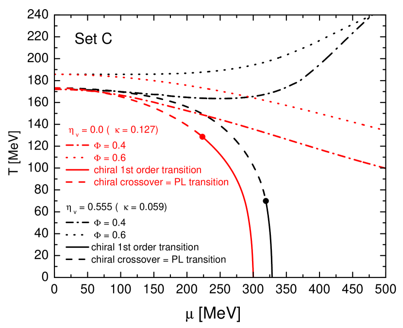
Figure 7: Phase diagrams with (pseudo)critical temperatures $T_{c}(\mu)$ and critical endpoints for set C parametrization of the nonlocal rank-2 PNJL model for the two cases $\eta_{v}=0.0$ and $\eta_{v}=0.555$. Dashed (full) lines correspond to the chiral crossover (first order) transitions. The PL transition lines, defined by the peak of the PL susceptibility, coincide with the chiral crossover. The dash-dotted and dotted lines represent the deconfinement transition range, i.e. $\Phi=0.4$ and $\Phi=0.6$, respectively.

The values for $T_{c}(\mu=0)$ (in MeV) are 169.9, 171.3, 173.2 and 200.9, for Sets A, B, C and local, respectively. These results indicate that the $T_{c}(0)$ of nonlocal covariant PNJL models is rather insensitive to the choice of the form factors parametrizing the momentum dependence (running) of the dynamical mass function and the WFR function of the quark propagator as measured on the lattice at zero temperature Parappilly:2005ei , whereas the position of the CEP and critical chemical potential at $T=0$ strongly depends on it.

In view of this finding, the absence of a CEP reported in the local limit Bratovic:2012qs as well as the result for Set A without WFR seems to be less realistic (see Ref.Contrera:2012wj ).

On the other hand, more recent lattice results Bellwied:2015rza ; Bonati:2015bha (LR II) suggest higher values for the $\kappa$ coefficient, which implies a lower or even vanishing vector coupling parameter $\eta_{V}$, giving better agreement for $\Delta P/T^{4}$ vs. $T/T_{c}$.

Considering the different lattice constraints for $\kappa$ and that the best fitting rank-2 nonlocal PNJL model is the one with Lorentzian form factors (Set C parametrization), the region in the QCD phase diagram where the CEP should be located according to our study, would be determined as $(T_{\rm CEP},\mu_{\rm CEP})=(128.6~{}{\rm MeV},223.3~{}{\rm MeV})$ for $\eta_{V}=0.0$ and $(T_{\rm CEP},\mu_{\rm CEP})=(69.9~{}{\rm MeV},319.1~{}{\rm MeV})$ for $\eta_{V}=0.555$. This region is highlighted in Fig. 7.

With this result of the present study we arrive at our conclusion for the NICA experiments which are devoted to the study of the quark-hadron mixed phase that shall be located at $T<T_{\rm CEP}$ and $\mu>\mu_{\rm CEP}$. We shall estimate whether the planned energy ranges of the BM@N experiment ($E_{\rm lab}=2-4$ A GeV) and of the MPD experiment ($\sqrt{s_{NN}}=4-11$ GeV) are suitable for accessing the region of the mixed phase that follows from our study. To this end we use a parametrization for the chemical freeze-out temperature in the QCD phase diagram by Andronic et al. Andronic:2005yp

$$T_{\rm freeze}=T_{\rm lim}\left(1-\frac{1}{0.7+[\exp(\sqrt{s_{NN}}({\rm GeV}))-2.9]/1.5}\right)$$ (23)

as obtained from statistical model analyses of hadron production in heavy-ion collision experiments, with $T_{\rm lim}=161\pm 4$ MeV. According to this parametrization and to the LR-I motivated nonlocal PNJL model with vanishing vector coupling, one should expect signals of a first order phase transition in collisions with $\sqrt{s_{NN}}\mathrel{\hbox to0.0pt{ \lower 4.0pt\hbox{\hskip-3.0pt$\sim$}\hss}\raise 1.0pt\hbox{$<$}}6$ GeV, right in the middle of the MPD energy scan. For the LR-II motivated parametrization with $\eta_{V}=0.555$ the CEP is at such a low temperature that only the BM@N experiment has a chance to access the mixed phase, at laboratory energies $E_{\rm lab}\mathrel{\hbox to0.0pt{ \lower 4.0pt\hbox{\hskip-3.0pt$\sim$}\hss}\raise 1.0pt\hbox{$<$}}3$ A GeV, within the range of this fixed target experiment but too low for the collider experiment MPD.

The main conclusion of this study is that for the search of CEP signatures and the investigation of properties of the quark-hadron mixed phase in BES programmes the energy range of the NICA and FAIR facilities shall be particularly promising. We find a certain preference for a CEP position at a critical temperature $T_{\rm CEP}\sim 130$ MeV, expected to be crossed in collisions with $\sqrt{s_{NN}}\sim 6~{}$GeV, corresponding to $E_{\rm lab}\sim 18~{}$A GeV. This energy could not be reached from above by the present RHIC BES programme of the STAR experiment (lower limit $\sqrt{s_{NN}}=7.7~{}$GeV and also not in the NA49 experiment at CERN SPS (lower limit $E_{\rm lab}=20~{}$A GeV). Just the ongoing NA61-SHINE experiment has a lower limit of $E_{\rm lab}=13~{}$A GeV in their energy scan that would allow to cross this suspected critical point (unless it would be located at slightly lower temperature). The old AGS experiment at BNL did not quite reach this energy (maximum energy $E_{\rm lab}=10.74~{}$A GeV) and were also not designed for a CEP search, while the energies at the GSI SIS are probably too low to reach the phase transition border (maximum energy $E_{\rm lab}=2~{}$A GeV). The theoretical investigation of the baryon stopping as a probe of the onset of deconfinement in heavy-ion collisions Ivanov:2012bh has revealed a characteristic ”wiggle” structure in the curvature of the proton rapidity distribution at $\sqrt{s_{NN}}\sim 6~{}$GeV which remains robust also when applying acceptance cuts of the MPD experiment Ivanov:2015vna at NICA. The MPD experiment at NICA will be the first dedicated heavy-ion collision experiment of the third generation to fully cover the suspected location of the CEP and thus to enter the mixed phase region via a first order phase transition. Contrary to studies with the local NJL model which first in Sasaki:2006ws and more recently in Bratovic:2012qs have shown that a CEP may be absent at all in the phase diagram for finite coupling in the repulsive vector channel, the present work with nonlocal PNJL models constrained by lattice QCD propagator data has shown that the presence of a CEP in the QCD phase diagram is rather robust against even stronger vector channel interactions.

Finally, we would like to mention currently ongoing developments of our approach to the QCD phase diagram and the EoS of matter under extreme conditions:

• Extension of the model to 2+1 flavours in order to properly compare with modern lattice QCD results Borsanyi:2013bia ; Bazavov:2014pvz .

• Investigation of the robustness of the results of the nonlocal PNJL models when modifying the choice of the Polyakov-loop potential taking into account recent developments Sasaki:2012bi ; Ruggieri:2012ny ; Fukushima:2012qa .

• Addition of quark pair interaction channels and the possibility of color superconducting quark matter phases GomezDumm:2008sk ; Blaschke:2010ka

• Going beyond the mean field approximation within the Beth-Uhlenbeck approach Blaschke:2013zaa , where hadronic correlations of quarks are included with their spectral weight showing both, bound and scattering parts, with a characteristic medium dependence that exhibits the Mott transition (dissociation of hadronic bound states into the scattering continuum at finite temperatures and chemical potentials).

A key quantity for such studies are is hadronic phase shifts. First results using a generic ansatz Blaschke:2015nma for joining the hadron resonance gas and PNJL approaches are promising Dubinin:2015glr . The inclusion of baryonic correlations is possible and has been started at finite temperatures Blaschke:2015sla and will be extended to the full phase diagram. As the behavior of the hadronic spectral functions and in particular the location of the Mott transitions in the QCD phase diagram is essentially determined by the dynamical quark mass functions, a key issue for future research is to investigate the backreaction of hadronic correlations on these order parameters. We expect that by following the Beth-Uhlenbeck approach one will have a methodic basis for answering the question about the robustness of predictions for the structure of the QCD phase diagram at the meanfield level discussed here.

References

- (1) M. A. Stephanov, PoS LAT 2006, 024 (2006).
- (2) A. Bazavov, T. Bhattacharya, M. Cheng, C. DeTar, H. T. Ding, S. Gottlieb, R. Gupta and P. Hegde et al., Phys. Rev. D 85, 054503 (2012).
- (3) N. M. Bratovic, T. Hatsuda and W. Weise, Phys. Lett. B 719, 131 (2013).
- (4) S. Carignano, D. Nickel, and M. Buballa, Phys. Rev. D 82, 054009 (2010).
- (5) M. Kitazawa, T. Koide, T. Kunihiro and Y. Nemoto, Prog. Theor. Phys. 108, 929 (2002).
- (6) D. Blaschke, M. K. Volkov and V. L. Yudichev, Eur. Phys. J. A 17, 103 (2003).
- (7) T. Hatsuda, M. Tachibana, N. Yamamoto and G. Baym, Phys. Rev. Lett. 97, 122001 (2006).
- (8) D. Blaschke, H. Grigorian, A. Khalatyan and D. N. Voskresensky, Nucl. Phys. Proc. Suppl. 141, 137 (2005).
- (9) A. Andronic, D. Blaschke, P. Braun-Munzinger, J. Cleymans, K. Fukushima, L. D. McLerran, H. Oeschler and R. D. Pisarski et al., Nucl. Phys. A 837, 65 (2010).
- (10) G. A. Contrera, D. Gomez Dumm and N. N. Scoccola, Phys. Lett. B 661 (2008) 113.
- (11) G. A. Contrera, M. Orsaria and N. N. Scoccola, Phys. Rev. D 82, 054026 (2010).
- (12) D. Horvatic, D. Blaschke, D. Klabucar, O. Kaczmarek, Phys. Rev. D 84, 016005 (2011).
- (13) A. E. Radzhabov, D. Blaschke, M. Buballa and M. K. Volkov, Phys. Rev. D 83, 116004 (2011).
- (14) S. Benic, D. Blaschke, G. A. Contrera and D. Horvatic, Phys. Rev. D 89, no. 1, 016007 (2014).
- (15) S. Roessner, T. Hell, C. Ratti and W. Weise, Nucl. Phys. A 814, 118 (2008).
- (16) A. Dumitru, R. D. Pisarski and D. Zschiesche, Phys. Rev. D 72, 065008 (2005).
- (17) K. Fukushima and Y. Hidaka, Phys. Rev. D 75, 036002 (2007).
- (18) H. Abuki, M. Ciminale, R. Gatto, G. Nardulli and M. Ruggieri, Phys. Rev. D 77, 074018 (2008); H. Abuki, R. Anglani, R. Gatto, G. Nardulli and M. Ruggieri, Phys. Rev. D 78, 034034 (2008).
- (19) D. Gomez Dumm, D. B. Blaschke, A. G. Grunfeld and N. N. Scoccola, Phys. Rev. D 78, 114021 (2008).
- (20) V. A. Dexheimer and S. Schramm, Phys. Rev. C 81, 045201 (2010).
- (21) B. -J. Schaefer, J. M. Pawlowski and J. Wambach, Phys. Rev. D 76, 074023 (2007).
- (22) V. Pagura, D. Gómez Dumm and N. N. Scoccola, Phys. Lett. B 707, 76 (2012).
- (23) S. Noguera and N. N. Scoccola, Phys. Rev. D 78, 114002 (2008).
- (24) G. A. Contrera, A. G. Grunfeld and D. B. Blaschke, Phys. Part. Nucl. Lett. 11, 342 (2014).
- (25) D. B. Blaschke, D. Gomez Dumm, A. G. Grunfeld, T. Klähn and N. N. Scoccola, Phys. Rev. C 75, 065804 (2007).
- (26) K. Fukushima, Phys. Rev. D 77, 114028 (2008).
- (27) D. Gomez Dumm and N. N. Scoccola, Phys. Rev. C 72, 014909 (2005).
- (28) A. V. Friesen, Y. L. Kalinovsky and V. D. Toneev, Int. J. Mod. Phys. A 30, no. 16, 1550089 (2015).
- (29) M. B. Parappilly, P. O. Bowman, U. M. Heller, D. B. Leinweber, A. G. Williams and J. B. Zhang, Phys. Rev. D 73, 054504 (2006).
- (30) C. R. Allton, S. Ejiri, S. J. Hands, O. Kaczmarek, F. Karsch, E. Laermann and C. Schmidt, Phys. Rev. D 68, 014507 (2003).
- (31) Z. Fodor, S. D. Katz and K. K. Szabo, Phys. Lett. B 568, 73 (2003).
- (32) A. Ali Khan et al. [CP-PACS Collaboration], Phys. Rev. D 64, 074510 (2001).
- (33) O. Kaczmarek, F. Karsch, E. Laermann, C. Miao, S. Mukherjee, P. Petreczky, C. Schmidt, W. Soeldner and W. Unger, Phys. Rev. D 83, 014504 (2011).
- (34) R. Bellwied, S. Borsanyi, Z. Fodor, J. G nther, S. D. Katz, C. Ratti and K. K. Szabo, arXiv:1507.07510 [hep-lat].
- (35) C. Bonati, M. D Elia, M. Mariti, M. Mesiti, F. Negro and F. Sanfilippo, Phys. Rev. D 92, no. 5, 054503 (2015)
- (36) A. Andronic, P. Braun-Munzinger and J. Stachel, Nucl. Phys. A 772, 167 (2006).
- (37) Y. B. Ivanov, Phys. Lett. B 721, 123 (2013).
- (38) Y. B. Ivanov and D. Blaschke, Phys. Rev. C 92, no. 2, 024916 (2015).
- (39) C. Sasaki, B. Friman and K. Redlich, Phys. Rev. D 75, 054026 (2007)
- (40) S. Borsanyi, Z. Fodor, C. Hoelbling, S. D. Katz, S. Krieg and K. K. Szabo, Phys. Lett. B 730, 99 (2014).
- (41) A. Bazavov et al. [HotQCD Collaboration], Phys. Rev. D 90, 094503 (2014).
- (42) C. Sasaki and K. Redlich, Phys. Rev. D 86, 014007 (2012).
- (43) M. Ruggieri, P. Alba, P. Castorina, S. Plumari, C. Ratti and V. Greco, Phys. Rev. D 86, 054007 (2012).
- (44) K. Fukushima and K. Kashiwa, Phys.Lett. B 723, 360 (2013).
- (45) D. B. Blaschke, F. Sandin, V. V. Skokov and S. Typel, Acta Phys. Polon. Supp. 3, 741 (2010).
- (46) D. Blaschke, M. Buballa, A. Dubinin, G. Roepke and D. Zablocki, Annals Phys. 348, 228 (2014).
- (47) D. Blaschke, A. Dubinin and L. Turko, Phys. Part. Nucl. 46, no. 5, 732 (2015).
- (48) A. Dubinin, D. Blaschke and A. Radzhabov, J. Phys. Conf. Ser. 668, no. 1, 012052 (2016).
- (49) D. Blaschke, A. S. Dubinin and D. Zablocki, PoS BaldinISHEPPXXII , 083 (2015); [arXiv:1502.03084 [nucl-th]].