A study of the elements copper through uranium in Sirius A:
Contributions from STIS and ground-based spectra

Abstract

We determine abundances or upper limits for all of the 55 stable elements from copper to uranium for the A1 Vm star Sirius. The purpose of the study is to assemble the most complete picture of elemental abundances with the hope of revealing the chemical history of the brightest star in the sky, apart from the Sun. We also explore the relationship of this hot metallic-line (Am) star to its cooler congeners, as well as the hotter, weakly- or non-magnetic mercury-manganese (HgMn) stars. Our primary observational material consists of Hubble Space Telescope ($HST$) spectra taken with the Space Telescope Imaging Spectrograph (STIS) in the ASTRAL project. We have also used archival material from the $COPERNICUS$ satellite, and from the $HST$ Goddard High-Resolution Spectrograph (GHRS), as well as ground-based spectra from Furenlid, Westin, Kurucz, Wahlgren, and their coworkers, ESO spectra from the UVESPOP project, and NARVAL spectra retrieved from PolarBase. Our analysis has been primarily by spectral synthesis, and in this work we have had the great advantage of extensive atomic data unavailable to earlier workers. We find most abundances as well as upper limits range from 10 to 100 times above solar values. We see no indication of the huge abundance excesses of 1000 or more that occur among many chemically peculiar (CP) stars of the upper main sequence. The picture of Sirius as a hot Am star is reinforced.

1. Introduction

The history of matter is written in its abundance patterns–a plot of abundances versus mass number $A$, or atomic number $Z$. For example, the imprint of major nucleosynthetic processes is seen in the iron peak, and the local maxima due to the $r-$ and $s-$ (rapid and slow) processes. Throughout an abundance plot, the persistent odd-even alternation of abundances, is the imprint of nuclear processing.

The abundance patterns of stars more massive than the Sun have revealed a history of significant non-nuclear processes. An overall pattern discussed in the pioneering diffusion work of Michaud (1970) was a deficiency of typically abundant elements, such as helium (He, $Z$ = 2), carbon (C, $Z$ = 6), and oxygen (O, $Z$ = 8), with an excess of rare species, for example, beyond the iron peak–gallium (Ga, $Z$ = 31), strontium (Sr, $Z$ = 38), yttrium (Y, $Z$ = 39), or zirconium (Zr, $Z$ = 40). Additionally, violations of the ubiquitous odd-even effect were found in the Sr-Y-Zr triplet, and even on the iron peak, where manganese (Mn, $Z$ = 25) could be more abundant than iron (Fe, $Z$ = 26) or chromium (Cr, $Z$ = 24) (cf. Adelman, et al. (2006)).

More recently, fascinating abundance patterns apparently unrelated to nucleosynthesis or diffusion have been noted in such disparate objects as the $\lambda$ Bootis stars (Venn & Lambert, 1990), Herbig Ae (Cowley, et al., 2010; Folsom, et al., 2012), and post-AGB stars (Van Winckel, 2003). These objects sometimes show solar abundances of the lighter elements, with deficiencies of heavier ones.

For Sirius, as for most A-stars, abundances are generally known for most of the elements through zinc (Zn, $Z$ = 30). Beyond Zn, “islands of detectability” are found, for example at Sr, Y, and Zr, and at barium (Ba, $Z$ = 56) and some of the lighter lanthanide rare earths (e.g. lanthanium (La, $Z$ = 57) – gadolinium (Gd, $Z$ = 64)). This leaves much of the periodic table unexplored. Yet significant clues to the chemical history of stars like Sirius may lie in these poorly explored regions.

Lacuna in the abundance patterns occur for several reasons. Cosmic abundances generally decline with increasing $Z$, so we are less likely to see lines from heavier elements than from lighter ones. This trend may be compensated, when an atomic or ionic spectrum is simple, with most of the line strength concentrated in a few wavelengths. This is one reason for the islands of detectability. But the strongest lines of an atom or ion may fall in wavelength regions that are not commonly available. This happens for many of the elements in the right-hand part of the periodic table. Many strong lines fall in the satellite ultraviolet. While the International Ultraviolet Explorer (IUE) spectra provided coverage of much of this region for many stars, its noise and spectral resolution left much room for improvement.

One of the goals of the ASTRAL Cool Star Project (Ayres, 2010) was to provide high-quality spectra in the satellite ultraviolet from the STIS instrument of the $HST$. The current study is a part of an extension of that project to hotter stars.

2. Resume of past work

We build upon a significant body of work. Aller (1942) published curve of growth studies of abundances in both Sirius and $\gamma$ Geminorum, presaging the larger work of Kohl (1964a, b), based on numerous high-dispersion photographic spectra. Information for some 3650 lines was presented in the second reference, including a number of relevance to the current paper. In the English abstract of the first of these references, Kohl states that “Sirius tends to be a metallic line star.” Conti (1965) gives references to several early works that called attention to the similarity of Sirius’s abundances to those of Am stars. Hill & Landstreet (1993) compared abundances from spectral synthesis of high-resolution spectra of six superficially normal A-stars, including Sirius.

High-quality wavelength measurements were not made for Sirius in earlier work. Such measurements often indicate the relative contributions of blends in a simple way that is possible, but sometimes tedious from a detailed synthesis, with multiple identifications. Accurate stellar wavelengths are not a substitute for the impressive techniques typified by the work of Kurucz, and Castelli (cf. Castelli (2015)). But they are an important supplement. Most of the wavelengths in Kohl (1964b) are from the laboratory, while Aller’s are from $\gamma$ Geminorum or the Sun.

Subsequent studies of Sirius would use electronic detectors as well as observations from space. A recent, detailed abundance study of Sirius was by Landstreet (2011) (henceforth, JDL), to which we refer for an excellent summary of the Sirius system. Landstreet’s work is based on ESO Ultraviolet and Visual Echelle Spectrograph (UVES) (Bagnulo, et al., 2003), $COPERNICUS$ (Rogerson, 1987), and GHRS (Wahlgren et al, 1993) spectra. Detailed synthetic calculations, described in Furenlid, et al. (1995), and published in part as a special report were described by Kurucz & Furenlid (1979). Because of the rotational velocity of Sirius ($v_{{\mathrm{e}}}\sin i=16$ km s^-1) the effective resolution of $COPERNICUS$, GHRS, and STIS spectra are comparable.

Sirius was included among the A-type stars studied by Lemke (1989, 1990). He determined abundances, using LTE and NLTE methods for C, Fe, Ti, Si, Ca, Sr, and Ba. More recently, Takeda, et al. (2008), gave abundances of C , O , silicon (Si, $Z$ = 14), titanium (Ti, $Z$ = 22), Fe , and Ba in 46 A-type stars. Takeda, et al. (2012) subsequently determined NLTE abundances of lithium (Li, $Z$ = 3), sodium (Na, $Z$ = 11), and potassium (K, $Z$ = 19) in 24 sharp-lined A-stars, including Sirius. Earlier, Qiu, et al. (2001) had determined abundances of 23 elements in Sirius and Vega. Their work included Zn, in addition to the Sr, Y, Zr triplet, Ba and La.

Virtually all of the work cited was restricted to the elements lighter than copper (Cu, $Z$ = 29), and the islands of detectability. But efforts to explore the less accessible heavier elements in Sirius have been made, chiefly based on $COPERNICUS$ but also on $IUE$ spectra. A study very much in the spirit of the present work is that of Wahlgren & Dolk (1998), who investigated hot Am stars as a bridge between HgMn and ordinary Am stars. They noted explicitly the importance of very heavy elements (VHE) as a key to abundance patterns.

Sadakane, et al. (1988) used $COPERNICUS$ spectra to obtain an abundance excess of mercury (Hg, Z = 80) in Sirius, which we confirm. Subsequently, Sadakane (1991) computed equivalent widths in Sirius for all elements with $Z$ $>$ 40 listed by Kurucz & Peytremann (1975) (henceforth, KP), assuming solar abundances. He then reported abundances of molybdenum (Mo, $Z$ = 42), cadmium (Cd, $Z$ = 48), tungsten (W, $Z$ = 74), and lead (Pb, $Z$ = 82). We used the same features for these elements as Sadakane (1991), but with the advantage of more recent $gf$-values. Moreover, numerous atomic or ionic lines are now available that were not in Corliss & Bozman (1962), the resource used by KP for heavier atoms and ions.

Yushchenko & Gopka (2006) reported abundances for 16 elements from Cu to uranium (U, $Z$ = 92): Cu, Ga, Y, Zr, Mo, Cd, tin (Sn, $Z$ = 50), hafnium (Hf, $Z$ = 72), tantalum (Ta, $Z$ = 73), W, rhenium (Re, $Z$ = 75), osmium (Os, $Z$ = 76), mercury, lead (Pb, $Z$ = 82), thorium (Th, $Z$ = 90), and U. Like Sadakane’s work, this was based on $COPERNICUS$ spectra. Yushchenko and Gopka show a plot of their abundances versus $Z$, but their brief contribution does not include the lines used or designate any points as upper limits.

3. Observations

3.1. STIS spectra

The characteristics and operational capabilities of HST Space Telescope Imaging Spectrograph (STIS) have been detailed in a number of previous publications, especially Woodgate et al. (1998) and Kimble et al. (1998).

The STIS observations of Sirius were carried out over a three week period in 2014 March, as part of a larger project, The Advanced Spectral Library – Hot Stars (ASTRAL), whose aim was to collect high signal-to-noise, full UV coverage (1150–3100 Å) “atlases” of 21 representative bright early-type stars (types O–A) at the highest spectral resolution feasible with STIS, rivaling the quality of ground-based measurements routinely acquired in the optical and near-infrared. The specific observing scenario for Sirius was one of essentially three set programs for the ASTRAL Project, which were tailored for specific types of objects. The scenario – called 7-Samurai (7-S) – combined seven high- and medium-resolution echelle settings of STIS to achieve the highest spectral resolution ($R\equiv\lambda/\Delta\lambda\sim$110,000) in specific regions where important stellar, and especially the narrow interstellar, features are found; but medium resolution ($R\sim$30,000–45,000) over other parts of the spectrum where high-S/N might have been unobtainable otherwise (in the limited observing time, typically 12 orbits per target for the 7-S program).

Table 1HST STIS Observation Log for Sirius

Exp. No.	Mode/Setting	U.T. Start	$t_{\rm exp}$	Aperture	QF
(1)	(2)	(3)	(4)	(5)	(6)
Visit T0: 2014 March 9
1	E140H-1271	17:59	$1{\times}1500$	ND2	62
2	E140M-1425	19:08	$2{\times}1296$	ND3	61
3	E230M-1978	20:44	$2{\times}1296$	ND3	114
4	E230H-2713	22:19	$2{\times}1297$	ND3	106
Visit T2: 2014 March 21
1	E140M-1425	11:59	$1{\times}1519$	ND3	46
2	E230H-2463	13:10	$2{\times}1294$	ND3	86
3	E230H-2513	14:46	$2{\times}1297$	ND3	93
4	E230H-2912	16:22	$2{\times}1297$	ND3	110
Visit T1: 2014 March 30
1	E140H-1271	06:19	$1{\times}1500$	ND2	63
2	E140M-1425	07:30	$2{\times}1296$	ND3	60
3	E230M-1978	09:05	$2{\times}1296$	ND3	112
4	E230H-2713	10:41	$2{\times}1297$	ND3	109

Note. — Col.(4): $n{\times}t$ format indicates number of sub-exposures ($n$) and integration time per sub-exposure ($t$) in seconds. Col. (5): ND2 is the $0.2^{\prime\prime}{\times}0.05^{\prime\prime}$ ND aperture; ND3 is the $0.3^{\prime\prime}{\times}0.05^{\prime\prime}$ND aperture. These filtered slits have roughly 1% and 0.1% transmission, respectively, compared with the normal clear echelle apertures. Col. (6): QF is a quality factor, the signal-to-noise per spectral resolution element (resel) averaged over the high-sensitivity central region of the echellegram.

The STIS observing program for Sirius is summarized in Table 1. The 12 orbits were divided into three 4-orbit “visits,” carried out about 10 days apart. Visits 0 and 1 were identical, and led off in the first orbit with a standard CCD target acquisition using direct imaging (“MIRROR”) through the F25ND5 heavily-filtered aperture. This was followed by a dispersed-light “peak-up” (target centering via a raster search) in the $0.3{\times}0.05$ND (ND=3) slit again using the CCD, but now with the 4451 Å setting of the G430M first-order grating. Filling out orbit 1 was a 1.5 kilosecond (ks) high-resolution echelle exposure of the 1200–1350 Å region with E140H-1271 through the $0.2{\times}0.05$ND (ND=2) slit. Sirius is so bright in the UV that these heavily-filtered slits (transmissions of 1% and 0.1% for ND2 and ND3, respectively) must be used even for the highly dispersed echelle spectroscopy. The relative slit positions are known accurately enough that a peak-up in ND3 can be transferred to an ND2 spectral observation. In the second orbit, a pair of 1.3 ks exposures was taken, covering the broader FUV band 1150–1700 Å with a medium-resolution echelle E140M-1425, now through the ND3 slit (which also was used for all the subsequent exposures). The third orbit was similar, again with a pair of 1.3 ks exposures, but switching to the NUV (1700–3100 Å) with medium-resolution grating setting E230M-1978, whose coverage is 1600–2400 Å. Finally, in orbit 4 a pair of 1.3 ks exposures was taken with the high-resolution NUV setting E230H-2713, which covers the range 2580–2830 Å, capturing important interstellar absorptions of Fe ii  near 2600 Å and Mg ii  near 2800 Å, among the more numerous stellar lines.

Visit 2 began with the same CCD imaging acquisition and ND3 slit peak-up as visits 0 and 1, but the orbit 1 exposure now was with the medium-resolution echelle E140M-1425 and ND3 slit, for 1.5 ks. Orbits 2-4 were devoted to NUV high-resolution settings E230H-2463, E230H-2513, and E230H-2912, one orbit each and again split into equal-length sub-exposures of 1.3 ks, and all through ND3. The latter two settings overlap with the blue and red ends of E230H-2713, respectively, boosting exposure in the Fe ii  and Mg ii  interstellar intervals. The E230H-2463 setting almost completely overlaps with E230H-2513, and the combination was treated effectively as a single setting; however, E230H-2463 extends just enough to the blue to join the red end of E230M-1978, to ensure spectral continuity through the NUV.

The full-orbit exposures (i.e., in orbits 2–4 of a visit) were broken into two equal-length sub-exposures in an effort to counteract “breathing” effects: the telescope focus can change slightly in response to thermal cycling and cause the image at the STIS slit focal plane to blur somewhat, possibly affecting the throughput, and in extreme cases inducing undesirable spectral “tilts.” This effect is of particular concern when very narrow slits are used, such as the ND2 and ND3 utilized exclusively for the Sirius program. To monitor the breathing effect, a quality factor (“QF” in Table 1) was calculated for each exposure by determining the total net counts (from the CALSTIS pipeline x1d file) in the central roughly two-thirds of the echelle pattern, then dividing by the number of independent resolution elements (resel) per (truncated) echelle order (1 resel$\sim 2$ spectral bins in the $1024{\times}1024$ image format) and by the number of echelle orders. The resulting quantity is the average number of net counts per resel for that exposure. The square root of that value then is approximately the S/N per resel, which was adopted as the quality metric. A large difference between the QF values of same-setting sub-exposures in an orbit would signal – in the absence of rapid stellar variability, certainly not anticipated for a star like Sirius – a change in the throughput due to focus variations. In the specific example of Sirius, most of the exposure pairs showed some evidence of these breathing effects, and it always was the case that the second sub-exposure exhibited higher throughput than the first, on average by a factor of 1.36${\pm}$0.06. An important side effect of the focus-related throughput variations is a slight tilting of the spectrum, because the telescope point spread function is wavelength dependent, which becomes most conspicuous in the settings that cover the most spectral territory (e.g., E230M-1978). These spectral tilting effects must be specially compensated in the spectral post-processing.

The STIS echellograms of Sirius were initially processed through the normal CALSTIS pipeline to yield the so-called x1d file, a tabulation of fluxes and photometric errors versus wavelength for each of the up to several dozen echelle orders of a given grating setting. This file then was subjected to a number of post-processing steps to: (1) correct the wavelengths for small errors in the pipeline dispersion relations; (2) de-tilt the spectra, as necessary, based on a polynomial correction derived relative to the highest throughput sub-exposure of a set (considering all the visits for a given target); (3) adjust the echelle sensitivity (“blaze”) function empirically based on achieving the best match between fluxes in the overlap zones between adjacent orders; and (4) merge the overlapping portions of adjacent echelle orders to achieve a coherent 1-D spectral tracing for the specific sub-exposure of that setting. Then followed a series of steps to merge the up to several independent (visit-level) exposures in a given setting, and finally splice these into a full-coverage UV spectrum of the object. An early description of these protocols, for the STIS StarCAT catalog, has been provided by Ayres (2010); but the most recent incarnation, including a number of key changes and improvements, is described on the ASTRAL site mentioned earlier. A fundamental component of the new ASTRAL protocols, as in the earlier StarCAT version, is a bootstrapping approach to provide a precise relative, and hopefully also accurate absolute, wavelength scale; and similarly for the stellar energy distribution. However, with the extensive use of the ND filters for Sirius, the absolute flux scale might not be as accurate as for another target for which the normal clear apertures, better-calibrated and less-affected by breathing, could be used.

3.2. Ground-based spectra

In addition to the STIS observations, we made use of the UVES and Kurucz-Furenlid spectra noted in Section 2. Characteristics of this material are given in the references cited there. Because the Kurucz-Furenlid spectra were photographic, while the UVES reduction was not optimal, especially for the longer wavelengths, we also used NARVAL I spectra downloaded from the PolarBase (Petit, et al., 2014) site. This material is described in detail by (Silvester, et al., 2012).

4. Identifications, abundances, and upper limits

4.1. Wavelengths and preliminary identifications

Measured stellar wavelengths, and tentative identifications are available for STIS spectra from 1300.28 to 1999.90 Å, and 2000.34 to 3044.87 Å.
Unlike the wavelengths in the papers cited in Section 2, these wavelengths were measured directly from the STIS spectrum independently of individual laboratory or Ritz wavelengths. They are therefore suitable to help decide if an absorption minimum may be attributed primarily to a single atomic or ionic line. Preliminary or tentative identifications were made with the help of predicted line depths from the VALD3 (Ryabchikova, et al., 2015) “extract stellar” option, which was supplied with $T_{\rm eff}=9900$K and $\log(g)=4.3$ from JDL. We enhanced those abundances, often by a factor of 3 so that lines from exotic species would not be dropped from the calculation as too weak. In subsequent abundance calculations, we used the same $T_{\rm eff}$ and $\log(g)$, but with JDL’s abundances, unenhanced.

A total of 5137 STIS wavelengths between 2000.34 and 3044.87 Å  were measured. The measurements were made line-by-line with the help of a visual display of the normalized spectra. A cursor was set near minima and a 5-point least-square parabola fit to the surrounding points. The adopted wavelength is the minimum of the parabola. For features in the shoulders of lines, or where no minimum was seen, the cursor was set at an (subjective) estimate of where the minimum might be. The position nearest the cursor was then taken for the wavelength.

We typically consider a deviation of up to 0.02 Å  of a stellar line from a laboratory position to be within the error of measurement, or to be caused by a minor blend. Larger deviations are taken to indicate more serious blending. Quite often, especially in the ultraviolet, many features will be very close blends–within $\pm$ 0.02 Å–often of a relatively strong line, e.g. Fe ii, with a line of interest. An abundance worker would usually ignore such features, and seek more favorable lines. In our cases, we sometimes have no alternative than to consider that the line of interest may still make a detectable contribution to the absorption, and try to determine what it might be.

In many cases, there was no indication of the presence of the feature sought, and only an upper limit was assigned. We will comment on the value of an upper limit determination below (Section 7).

Few should doubt that atoms of all of the stable elements from Cu and Bi, as well as U and Th are present at some level in the atmosphere of Sirius. Some elements may have only lines below our current threshold of detectability. In this work, we may provide at least minimal information on such elements by reporting upper limit estimates. Additionally, we relax the usual criteria for making line identifications and/or abundance determinations. We accept that some atomic or ionic lines may make contributions to the absorption without having a close, measurable wavelength minimum. This method is not new, and is commonly used when abundances are determined by spectrum synthesis from spectra that are blended by large values of $v_{{\mathrm{e}}}\sin i$.

4.2. Analysis

Our abundance analyses have all used spectral synthesis based on a model atmosphere with temperature, gravity, and abundances adopted by JDL. The models assumed hydrostatic and radiative equilibrium, and LTE, and are essentially ATLAS9 models (Castelli & Kurucz, 2003; Kurucz, 2015). In lieu of a lengthy description and comparison of individual techniques, we list in Table  2 representative papers where the different techniques have been used. For the elements studied by two or more authors, many cross checks were carried out to prevent errors that could arise from a variety of causes, such as misidentification of contributors to blends, misplacement of continuua, or poor atomic data.

Table 2Codes and relevant references

Author	Code(s)	Reference
CRC	ATLAS9/DYNTHL	Cowley, et al. (2010)
FC	ATLAS9/SYNTHE	Castelli (2015)
AFG	ATLAS9/SYNSPEC49/
	STELLAR	Hill, et al. (2010)
RM	ATLAS9/SYNSPEC48/
	ROTIN3	Kiliçoğlu, et al. (2016)
GMW	ATLAS9/SYNTHE	Wahlgren, et al. (1997)

For the elements considered, we have synthesized the region of one or more of the strongest available lines. These were typically chosen with the help of the NIST online Handbook (Sansonetti, Martin & Young, 2005). We also examined the output from VALD3’s (Ryabchikova, et al., 2015) “extract stellar” option, which was supplied with the model and abundances of JDL. Each of these sources has a distinct advantage. The VALD3 output supplies likely blends, along with an estimate of their strengths. But in the STIS region, a number of important lines have antiquated oscillator strengths. In a few cases, there were no data in VALD3, and the corresponding lines could not be in the originally computed spectra. Examples are for singly-ionized antimony (Sb, $Z$ = 51) and tellurium (Te, $Z$ = 52).

Typically, our synthesis would proceed with an assumed abundance of the element that was 2 dex (and sometimes more) higher than the solar value. This was useful to show clearly where a line would occur in a region with complex blending, because the line of interest would be “overpredicted,” that is stronger than the observed spectrum. The abundance would then be reduced to “fit” the observation.

All calculations have been made in LTE, with default broadening parameters. Hyperfine structure or isotope shifts were included in calculations for Cu, I, Eu, Re, Hg, Tl, and Bi. Typically, the abundances were lower when these effects were included, by 0.2 to 0.5 dex.

4.3. Oscillator strengths and partition functions

Oscillator strengths for the 55 individual target elements were obtained with the help of references from the NIST online database (Kramida, et al., 2014). Sources for oscillator strengths are listed in Table 3. A glance at the publication dates of these references shows that most of this work was unavailable to the researchers mentioned in Section 2. In a few cases, we were unable to find satisfactory values, and have used ad hoc determinations (this paper), as follows:

• For Sb ii  at 1387.56 Å, the Cowan code (Cowan, 1981) was used to obtain $\log(gf)=-0.34$.

• For the line of singly-ionized cesium (Cs, $Z$ = 55), Cs ii  at 4603.79 Å, we used the value $\log(gf)=0.4$, based on an analogous transition in Kr i, at 8113 Å  ($5s-5p$).

For background or blending lines, $gf$-values came from VALD3 or the Kurucz website (Kurucz, 2013). Differences in these sources were occasionally of significance and were adjusted so that authors used the same values.

Partition functions occasionally needed reconcilation among workers. The main sources for the heavy elements were the block data segments from the SYNTHE code (Kurucz, 2015) or assembled independently by CRC ( Cowley, cf. Cowley, et al. (2003)).

4.4. Grades of determinations

The analysis performed with the different codes and line lists given in Table 2 has shown that abundances for Cu, Zn, elements in the islands of detectability (Sr, Y, Zr, Ba), Br, Ce, and Pr may be considered known to 0.2 dex or better. Abundances for Sr, Y, Zr, and Ba were redetermined in the present work. They agreed to 0.05 dex or better, with those of JDL (Column L11 of his Table 1).

The measured wavelengths played an important role in our assessment of the quality of an abundance determination. When the wavelengths are close to the laboratory positions, and some 80% or more of the absorption is due to the element in question, abundances are assigned a ‘g’ for good. However, in some cases, such as Mo or Nd, the uncertainties range up to 0.3 dex, because of difficulties with continuum location, blends, or oscillator strengths.

When there is no absorption minimum within 0.02 Å, but calculations show that roughly half of the absorption is due to the element in question, we assign a grade of ‘f’ for fair. An example of such a fit is at 1414.40 Å  of Ga ii. In the remainder of cases, we assign a grade of poor, ‘p’, or an upper limit ‘ul’. We consider the abundance uncertainties in the ‘f’ to ‘p’ categories to range up to 0.5 dex.

5. Results

Table 3Brief tabulation of results

Spect	$\lambda$(Å)1	$\lambda^{*}$(Å)2	Q	[El/H]	Sun3	$\log(gf)$	$gf$–Ref.
Cu i	3273.96	73.98	g	+0.7	4.18	$-0.359$	Liu, et al. (2014)
Zn i	4722.16	22.19	g	+1.1	4.56	$-0.39$	Biémont & Godefroid (1980)
Ga ii	1414.40	14.39	f	+0.7	3.02	$+0.25$	Shirai, et al. (2007)
Ge ii	1649.19	49.22	f	+0.5	3.63	$-0.28$	Fuhr & Wiese (2005)
As ii	1375.07	nmb	ul	+1.8	2.30	$-0.632$	Biémont, et al. (1998a)
Se i	1960.89	60.85	p	+0.6	3.34	$-0.434$	Morton (2000)
Br i	1488.45	88.43	g	+1.3	2.54	$-0.58$	Morton (2000)
Kr i	8776.75	nm	ul	+3.	3.25	$+0.19$	Fuhr & Wiese (1996)
Rb i	7947.60	nm	ul	+1.7	2.47	$+0.14$	Morton (2000)
Sr ii	4077.71	77.72	g	+0.7	2.83	$+0.15$	Fuhr & Wiese (1996)
Y ii	3600.73	00.73	g	+0.7	2.21	$+0.34$	Biémont, et al. (2011)
Zr ii	3391.97	91.97	g	+0.7	2.59	$+0.57$	Ljung, et al. (2006)
Nb ii	3215.59	nm	ul	+1.	1.47	$-0.24$	Nilsson, et al. (2010)
Mo ii	2020.31	20.30	g	+1.0	1.88	$+0.022$	Silkstrom, et al. (2001)
Ru ii	1875.56	75.54	p	+1.0	1.75	$-0.23$	Palmeri, et al. (2009)
Rh ii	1634.72	nm	ul	+1.5	0.89	$-0.93$	Quinet, et al. (2012)
Pd ii	2488.91	nm	ul	+1.5	1.55	$+0.40$	Quinet (1996)
Ag ii	2246.41	nm	ul	+1.1	0.96	$+0.42$	Kramida (2013)
Cd ii	2265.02	65.01	g	+0.7	1.77	$-0.34$	Glowacki & Migdalek (2009)
In ii	1586.37	86.33	ul bl	+1.8	0.80	$+0.14$	Curtis (2000)
Sn ii	1899.97	99.90	p bl	+0.7	2.02	$-0.22$	Oliver & Hibbert (2010)
Sb ii	1387.56	nm	ul	+1.3	1.01	$-0.337$	see Sec. 4.3
Te ii	1461.68	61.57	ul	+1.	2.18	$-0.74$	Zhang, et al. (2013)
I i	1457.98	57.98	g	+2.0	1.55	$+0.20$	Chang, et al (2010)
Xe i	1469.61	nm	p	+1.1	2.24	$-0.58$	Morton (2000)
Cs ii	4603.79	nm	ul	+3.8	1.08	$+0.40$	see Sec. 4.3
Ba ii	4554.03	54.05	g	+1.4	2.25	$+0.14$	Klose, et al. (2002)
La ii	4042.91	nm	f	+1.5	1.11	$+0.33$	Zhiguo, et al. (1999)
Ce ii	4460.21	nm	g	+1.5	1.58	$+0.28$	Lawler, et al. (2009)
Pr ii	4222.93	nm	g	+2.2	0.72	$+0.27$	Biémont, et al. (2003)
Nd iii	5294.10	nm	g	+1.4	1.42	$-0.69$	Ryabchikova, et al. (2006)
Sm ii	3568.27	nm	f	+2.	0.95	$+0.29$	Lawler, et al. (2008a)
Eu ii	4205.05	nm	f	+1.3	0.52	$+0.21$	Lawler, et al. (2001a)
Gd ii	4251.73	51.76	p	+1.6	1.08	$-0.22$	Den Hartog, et al. (2006)
Tb ii	3509.15	nm	p	+2.	0.31	$+0.70$	Lawler, J. E. (2001b)
Dy ii	3531.70	31.61	p	+1.7	1.10	$+0.77$	Wickliffe, et al. (2000)
Ho ii	3456.02	nm	ul	+1.8	0.48	$+0.76$	Lawler, et al. (2004)
Er ii	3499.10	nm	f	+1.8	0.93	$+0.29$	Lawler, et al. (2008)
Tm ii	3462.20	nm	ul	+2.1	0.11	$+0.03$	Wickliffe & Lawler (1997)
Yb ii	3289.37	89.39	ul	+1.8	0.85	$-0.05$	Biémont, et al. (1998b)
Lu ii	2615.42	15.42	f	+1.6	0.10	$+0.14$	Quinet, et al. (1999)
Hf ii	2647.29	nm	ul	+1.8	0.85	$+0.46$	Bouazza, et al. (2015)
Ta ii	2400.13	00.03	ul	+1.7	$-$0.12	$+1.65$	Corliss & Bozman (1962)
W ii	2029.99	29.96	p	+1.5	0.83	$+0.18$	Nilsson, et al. (2008)
Re ii	2275.25	nm	ul	+1.7	0.26	$-0.385$	Ortiz, et al. (2013)
Os ii	2194.39	94.41	f	+1.0	1.40	$-0.22$	Quinet, et al. (2006)
Ir ii	2126.81	26.85	ul	+1.0	1.42	$+0.11$	Xu, et al. (2007)
Pt ii	1883.06	83.04	f	+1.6	1.62	$-0.12$	Quinet, et al. (2008)
Au ii	2082.07	82.05	f	+1.5	0.91	$-0.09$	Fivet, et al. (2006)
Hg ii	1942.27	42.31	g	+1.2	1.17	$-0.418$	Proffitt, et al. (1999)
Tl ii	1321.64	21.68	f	+0.9	0.90	$+0.12$	Curtis (2000)
Pb ii	2203.53	03.49	f	+1.4	1.92	$-0.143$	Morton (2000)
Bi ii	1791.84	nm	ul	+1.6	0.65	$-0.51$	Palmeri, et al. (2001)
Th ii	4019.13	nm	ul	+1.5	0.03	$-0.23$	Nilsson, et al. (2002a)
U ii	4241.66	nm	ul	+3.	$-$0.54	$-0.10$	Nilsson, et al. (2002b)

Table 3 is a concise summary of our results for the 55 elements. The elemental abundances are given as logarithmic ratios of elements-to-hydrogen, on the astronomical scale where $\log(H)=12$. All entries in the column labeled [El/H] were newly determined in the present work.

The solar abundances are from recent updates of Scott, et al. (2015), and Grevesse, et al. (2015). For elements not in these updates, values were taken from Asplund, et al. (2009), Table 1. Meteoritic abundances assigned by Asplund, et al. (2009) were used when photospheric values were not available. Of the 14 abundance results considered good (g), most are for species determined by other workers, notably JDL, or Sadakane (1991). Twelve of the abundances are considered fair (f), while eight are marked poor (p). For 21 elements, we give only upper limits (ul).

Space does not permit a discussion of 55 individual elements, but for a few elements we discuss specific cases, and examples are given for the various categories of quality. Detailed information for individual elements may be found on a website dedicated to the Sirius analysis: http://dept.astro.lsa.umich.edu/$\sim$cowley/Sirius/. Table 4 lists additional lines that were examined to support the abundances listed in Table 3.

In the sample plots of the following sections, the lines of the target elements typically have better fits than neighboring features. This happens primarily because (1) we select the regions best suited to the target element, and (2) for the latter, we adjust the abundance for an optimum fit. Random wavelengths especially in the ultraviolet, often have poor oscillator strengths. Additionally, these regions are replete with line absorption whose origin is not known.

5.1. Sample: Bromine (Br, Z = 35)

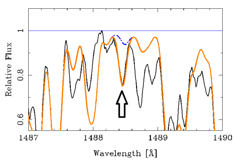
Figure 1.— Synthesis of the region near Br i  at 1488.45 Å. The broken (blue online) line was computed with a solar Br abundance. The gray (orange online) spectrum assumed an enhancement of 1.3 dex above solar. This determination is rated: ‘g’ (good).

Because Br has a first ionization energy of 11.8 eV, it is reasonable to expect the resonance lines of Br i  would appear. Lines at 1488.45 and 1540.65 Å  arise from the ground state.

Synthesis of the line at 1488 Å  is shown in Fig. 1. The broken (blue online) line was computed assuming a solar bromine abundance, while the gray (orange online) line was made assuming a 1.3 dex enhancement. The measured stellar wavelength was 1488.434 Å, and the synthesized fit is excellent. The oscillator strength is from Morton (2000). Of two possible lines that might confirm the identification, one, at 1540.65 Å  is at a region with missing absorption. However, there is no measured minimum at this wavelength, and additional contributors are needed to explain the absorption. Another line, at 1574.84 Å  is significantly weaker than the other two. Moreover, it is closely coincident with strong lines of Si i, measured at 1574.87 Å.

We conclude that the bromine abundance in Sirius is 1.3 dex above solar. The determination is graded ‘g’.

5.2. Sample: Gallium (Ga, $Z$ = 31)

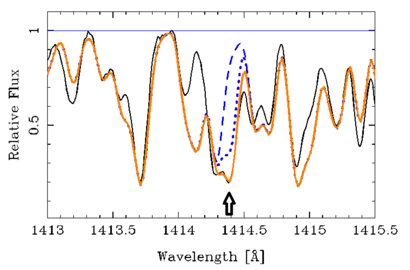
Figure 2.— Synthesis of the region near Ga ii  at 1414.40 Å. The dotted (blue online) line was computed with a solar Ga abundance. The dashed line was computed assuming no Ga at all. The gray (orange online) spectrum assumed an enhancement of 0.7 dex above solar. This determination is rated: ‘f’ (fair).

Fig. 2 shows the Ga ii  line at 1414.40 Å  closely blended primarily with Fe ii and Ni ii  on the short wavelength side. The minimum, indicated by the arrow, was measured at 1414.39 Å, in excellent agreement with the NIST wavelength. The solid gray (orange online) line was calculated with a Ga excess of 0.7 dex, while the dotted line shows the result for a solar abundance of gallium. For the dashed blue line, the Ga abundance was set to zero. Clearly a substantial portion of the absorption is due to Ga. We grade this determination ‘f’.

5.3. Sample: Ruthenium (Ru, $Z$ = 44)

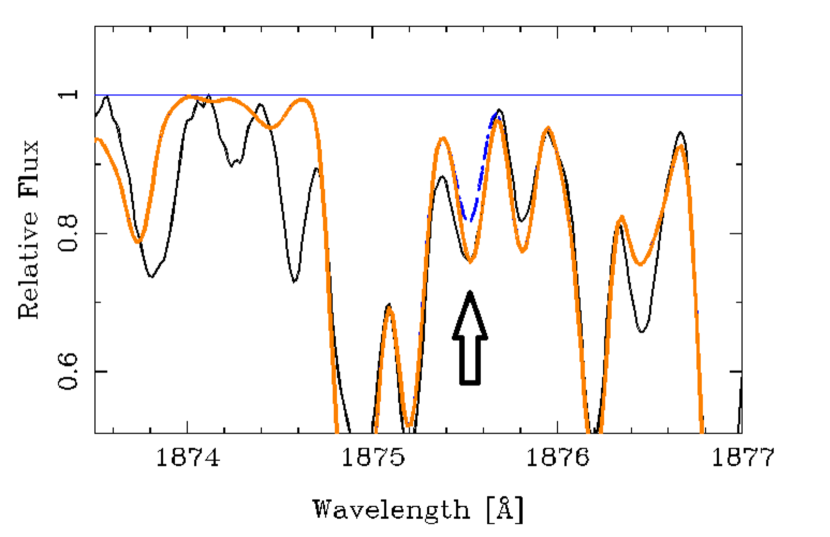
Figure 3.— Synthesis of the region near Ru ii  at 1875.56 Å. The Ru abundance is enhanced by 1.3 dex for the computed gray (orange online) spectrum. Zero Ru was assumed for the broken (blue online) spectrum. Syntheses near Ru ii  lines at 1939.04, 1939.51, 1966.07, and 1966.73 Å  give an average of 1.0 as the abundance excess. We rate the overall determination as ‘p’ (poor).

In Fig. 3, the arrow marks the position of the Ru ii  line, and the dashed (blue online) spectrum was calculated assuming no ruthenium at all. A solar abundance of ruthenium hardly changes the calculation from the dashed line. That is because of a relatively strong Fe ii  line at 1875.53 Å. VALD3 gives the source of the log($gf$) for Fe ii  as K13 (Kurucz, 2013). We find no other source for that line. If we use the default log($gf$)’s for the Fe ii  and Ru ii, the ruthenium abundance that fits gray (orange online) has an excess of 1.2 dex.

We examined the region near two other Ru ii  lines, at 1939.04 and 1939.51 Å. These led us to lower our estimate of the Ru abundance to +1.0 dex above the solar value. The determination is graded ‘p’.

5.4. Sample: Rhenium (Re, $Z$ = 75)

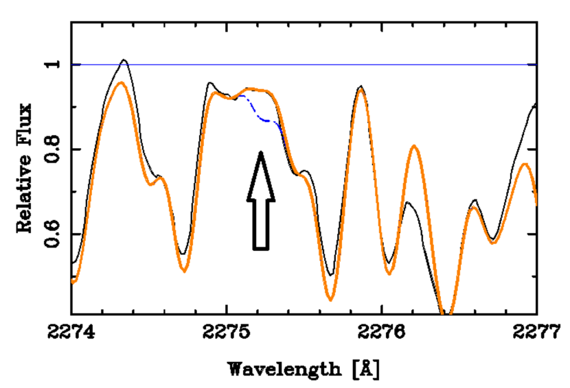
Figure 4.— Synthesis of the region near Re ii  at 2275.25 Å. The gray line (orange online) was made assuming an Re excess of 1.7 dex. The broken (blue online) was made assuming a 2.7 dex excess. The calculation includes full hyperfine structure. Only an ‘ul’ (upper limit) was assigned.

We found only an upper limit to the Re abundance. Figure 4 is illustrative of upper limits. The gray (orange online) line fits the observation roughly with an assumed Re excess of 1.7 dex. Since there is no observed minimum, we report 1.7 dex as the upper limit. The broken blue line was calculated assuming a 2.7 dex excess. Both calculations used the full hyperfine structure of the 2275 Å line as given by Wahlgren, et al. (1997).

5.5. Sample: Iodine (I, $Z$ = 53)

We are unaware of a credible identification of iodine in the spectrum of another star, and therefore highlight this result. This resonance transition is the analogue of the line for Br i.

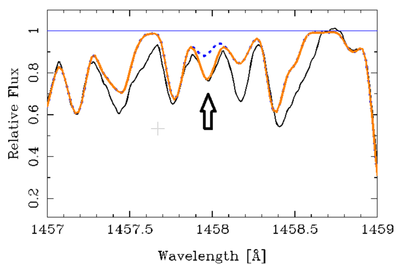
Figure 5.— Synthesis of the region near I i  at 1457.98 Å. The I abundance is enhanced by 2.0 dex for the gray (orange online) calculation. The broken spectrum (blue online) was made with solar abundance. The full 12-component hyperfine structure was included from Luc-Koenig, et al. (1975). This determination is rated ‘g’ (good).

Figure 5 shows I i  at 1457.98 Å. The stellar and laboratory wavelength measurements agree to 0.01Å. However, possible confirmation from expected lines at 1702.07, 1782.74 or 1830.38 Å  is unavailable because of blending. The fit shown in gray (orange online) was made with an excess of 2.0 dex. The abundance determination is graded ‘g’ based on our adopted criteria. The large abundance excess makes iodine an ostensible odd-Z anomaly. However, it is also possible that the oscillator strengths of closely blending lines of Fe ii, Mn ii, and Cr ii  are underestimates. This is likely because of the complex nature of the transitions themselves.

6. The abundance pattern of Sirius and its meaning

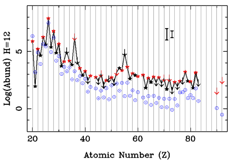
Figure 6.— Abundances (stars) and upper limits (arrows) for $\alpha$ CMa. Even-$Z$ elements are in red. Solar abundances are also shown(Sun symbols, blue online). Error bars are shown for quality good ($\pm 0.3$) and fair to poor ($\pm 0.5$ dex). These uncertainties do not apply to the upper limits.

Figure  6 shows the abundances and upper limits from Ca ($Z$ = 20) through U, along with the solar abundances. The latter fall typically 1 to 2 dex below those for Sirius. There are no indications of the 4 or more dex excesses found in the HgMn stars, apart, possibly, for Cs ($Z$ = 55).

The high upper limits at $Z$ = 36 and 55 are due to the atomic properties of Krypton (Kr $Z$ = 36) and Cs. The resonance lines of both Kr i, Kr ii, and Cs ii  fall in the far ultraviolet, short of our wavelength coverage. The Cs i  lines are accessible, but the ionization energy of neutral cesium is so low (3.89 eV) that observations of the neutral species are precluded in an A star. Thus, we cannot assume high upper limits to be likely abundance peaks, though we strictly cannot exclude that possibility. The point for I ($Z$ = 52) could indicate an odd-Z anomaly (cf. Section 5.5).

We see that a number of the exotic elements, that are often overabundant by 3 or more dex in HgMn stars, Ga, Au, Pt, Hg, fall smoothly among their neighbors. Pt and Pb have abundances 1.6 and 1.4 dex above their solar values.

For typical HgMn stars the Mn abundance increases with increasing temperature, while the platinum abundance has been found to be significantly anticorrelated with temperature (Smith & Dworetsky, 1993). If, as has been suggested (e.g. Adelman, et al. (2003)), the HgMn and Am stars are related, we might expect Pt to be unusually high in Sirius. Its $T_{\rm eff}=9900$K would place it at the cool end of the HgMn stars. For example, the Pt excess in the cool ($T_{\rm eff}=10750$K) HgMn star HR 7775 is 4.6 dex (Wahlgren, et al., 2000). We find only 1.6 dex for Sirius, a typical value for most of the heavy elements.

Unfortunately, our upper limits contain no information on possible underabundances. Perhaps the most notorious underabundance of the HgMn stars is that of Zn, which is some 4 orders of magnitude below the solar value in $\chi$ Lupi (Leckrone, et al., 1999), and only upper limits were reported for a number of HgMn stars by Smith & Dworetsky (1993). While a few HgMn and related stars have Zn excesses of 1 to 2 dex, as we find for Sirius, Zn in Sirius is not typical of most HgMn stars.

The STIS results are consistent with the prevailing interpretation of Sirius as a “hot Am” star, with underabundances of certain lighter elements, and mild excesses of heavier ones.

7. Comparison of observations to theoretical predictions

For nearly half a century, the (only) theory considered likely for abundance anomalies in all varieties of CP stars has been endogenous chemical separation–photospheric or sub-photospheric diffusion, or stellar winds (Alecian, Richard & Vauclair, 2005). The models upon which theoretical predictions are based have evolved significantly since the early 1970’s. In the beginning, a decisive factor was the ratio of upward (radiation, $g_{R}$) to downward (gravitational and thermal) forces in the outer stellar envelopes. In a figure that might have been relevant for the present paper, Michaud, et al. (1976) gave this ratio for elements with atomic numbers $Z$ through ca. 65, for stars of 1.2 through 3.3 $M_{\odot}$. The plots appeared to explain the underabundances of Ca and Sc in Am stars, but showed lack of support for Fe and Y, and Sr conflicting with the observation that these elements are typically overabundant in Am stars.

More recent calculations by Michaud, Richer & Vick (2011) (henceforth MRV) were made specifically for Sirius. Unfortunately, they extend only from He through Ni ($Z$ = 28). Unlike the calculations of the 1970’s, these predictions are based on chemical separations throughout the bulk of the star and as a function of age. Results are presented for two basic models, one with a turbulent envelope below a mixed outer mass of ca. $10^{-6}M_{\odot}$. A second model did not have turbulence in the envelope, but assumed a mass loss near $10^{-13}M_{\odot}$ year^-1. The predicted abundance patterns from the models are remarkably similar (see Figure 4 of MRV). The authors state that “Among the 17 abundances determined observationally, up to 15 can be predicted to within 2$\sigma$, and 3 of 4 determined upper limits are satisfied.” This is a “glass half full” conclusion.

A less favorable evaluation could come from a Chi-squared comparison. This would show that the deviations of JDL’s abundances, as cited earlier, from MRV’s predictions cannot be accounted for in terms of the abundance errors ($\leq 0.2$ dex). The Chi-squared sum would be dominated by the upper limit found for the element B ($Z$ = 5). That value alone would be sufficient to allow one to reject a null hypothesis that the deviations from theory are due only to observational errors. We find independently, an upper limit for B that is 1.45 dex below the predicted value. It is entirely valid to use this as an abundance with the understanding that a definite value would only increase the Chi-squared, making the null hypothesis even less acceptable.

MRV note the difficulty with B, and also one with Na. They suggest that mass transfer from the secondary could be relevant. Similar remarks were made by Richer, et al. (2000) and JDL, who also remarks that the separation of the two stars has “led people to assume that no important interaction occurred.”

8. Summary

In this work we have determined abundances for 34 elements from copper through uranium. Additionally, 21 upper limits were assigned. We are able to rule out the possibility that any elements (apart from Cs) have excesses of 4 dex or more. Abundance excesses of heavy elements fall generally between 1 and 2 dex. We find no clear violations of the odd-even effect as is found in some HgMn stars, for example, at yttrium. The most modern theoretical calculations (of MRV) relevant to Sirius do not cover elements examined here.

Appendix A Appendix: Lines examined

Table 4Additional lines used for abundances

Element	Spectrum	$\lambda$(Å)	$\lambda$(Å)	Element	Spectrum	$\lambda$(Å)	$\lambda$(Å)
Cu	i	3247.54		Zn	i	4680.14	4810.53
				Zn	ii	2025.48
Ga	iii	1495.04		Ge	i	2041.71	2068.66
	i	2094.26		As	i	1890.42	2860.44
Br	i	1540.65	1574.84	Rb	i	7800.27
				Rb	ii	4244.40
Sr	ii	4215.52		Y	ii	3242.27	3611.04
				Y	ii	3710.30
Zr	ii	3438.23	3479.39	Zr	ii	3496.21	3551.95
Nb	ii	2033.01	2697.03
Nb	ii	2109.43
Ru	ii	1939.04	1939.51
	ii	1966.07	1966.73	Rh	ii	2420.97
Cd	ii	2144.41		Sn	ii	1400.47
Sb	i	2068.33		Te	i	2002.03
				Te	ii	4654.37	5649.26
				Te	ii	5708.12
I	i	1702.07	1782.74	Xe	ii	5419.15
Ba	ii	4934.08		Ce	ii	4562.36
Pr	ii	4062.81
Pr	iii	5299.99		Nd	ii	4303.57
Sm	ii	3592.60		Eu	ii	4129.70
				Eu	iii	2375.46	2444.38
				Eu	iii	2513.76
Gd	ii	3545.80	3549.36
Gd	iii	2223.95	3545.80	Dy	ii	3436.02	3534.96
Ho	ii	3398.95	3796.75
Ho	ii	3810.74		Er	ii	3264.78	3372.71
				Er	ii	3616.56
Tm	ii	3131.26	3701.36
Tm	ii	3761.33		Yb	iii	2516.81
Lu	iii	2236.18	2603.35
Lu	iii	2911.39		Hf	ii	3399.79	3561.66
Ta	ii	2146.87		W	ii	1951.05
Re	ii	2608.50		Os	ii	2067.21	2070.67
				Os	ii	2282.26
Ir	ii	2169.42	2579.48	Pt	ii	1777.09	2144.25
Au	ii	1362.33		Hg	ii	1649.94
Tl	ii	1908.62		Pb	ii	1433.91	1822.05
Bi	ii	1436.81		Th	iii	1307.44	1356.92
U	ii	1358.57	4241.66	U	iii	3565.73

Most of the abundance results reported in Table 3 depend primarily on a single feature. But typically several features were examined for consistency with the adopted values. In Table 4, we list the wavelengths of the lines examined for each element that are not in Table 3.

References

- Adelman, et al. (2003) Adelman, S. J., Adelman, A. S. & Pintado, O. I. 2003, A&A, 397, 267
- Adelman, et al. (2006) Adelman, S. J., Caliskan, H., Gulliver, A. F. & Teker, A. 2006, A&A, 447, 685
- Alecian, Richard & Vauclair (2005) Alecian, G., Richard, O., and Vauclair, S. (eds) 2005, Element Stratification in Stars: 40 Years of Atomic Diffusion, EAS Pub. Ser. 17
- Aller (1942) Aller, L. H. 1942, ApJ, 96, 321
- Asplund, et al. (2009) Asplund, M., Grevesse, N., Sauval, J. 2009, ARAA, 47, 481
- Ayres (2010) Ayres, T. 2010, ApJS, 187, 149
- Bagnulo, et al. (2003) Bagnulo, S., et al. 1993, ESO Messenger, 114, 10
- Biémont & Godefroid (1980) Biémont, É. & Godefroid, M. 1980, A&A, 84, 361
- Biémont, et al. (1998a) Biémont, É., Morton, D. C. & Quinet, P. 1998, MNRAS, 297, 713
- Biémont, et al. (1998b) Biémont, É., Dutrieux, J.-F., Martin, I. & Quinet, P. 1998, J. Phys. B, 31, 3321
- Biémont, et al. (2003) Biémont, É., Lefèbvre, P.-H., Quinet, P., et al. 2003, Eur. Phys. J. D, 27, 33
- Biémont, et al. (2011) Biémont, É., Blagoev, K., Engström, L., et al. 2011, MNRAS, 414, 3350
- Bouazza, et al. (2015) Bouazza, S., Quinet, P. & Palmeri, P. 2015, JQSRT, 163, 39
- Castelli & Kurucz (2003) Castelli, F. & Kurucz, R. L. 2003, in Modelling of Stellar Atmospheres, IAU Symp. 210, ed. N. E. Piskunov, W. W. Weiss & D. F. Gray.
- Castelli (2015) Castelli, F. 2015, http://wwwuser.oats.inaf.it/castelli/hd175640/hd176540.html
- Chang, et al (2010) Chang, Z., Li, J. & Dong, C. 2010, J. Phys. Chem. A, 114, 13388
- Conti (1965) Conti, P. S. 1965, ApJ, 142, 1594
- Corliss & Bozman (1962) Corliss, C. H. & Bozman, W. R. 1962, Experimental Transition Probabilities for Spectral Lines of Seventy Elements, NBS Monog. 53 (CB)
- Cowan (1981) Cowan, R. D. 1981, The Theory of Atomic Structure and Spectra (Berkeley: Univ. Calif. Press)
- Cowley, et al. (2003) Cowley, C. R., Adelman, S. J. & Bord, D. J. 2003, in Modelling of Stellar Atmospheres, IAU Symp. 210, ed. N. Piskunov, W. W. Weiss & D. F. Gray, p. 261
- Cowley, et al. (2010) Cowley, C. R., Hubrig, S., González, J. F. & Savanov, I. 2010, A&A, 523, 65
- Curtis (2000) Curtis, L. J. 2000, Phys. Scr., 62, 31
- Den Hartog, et al. (2006) Den Hartog, E. A., Lawler, J. E., Sneden, C. & Cowan, J. J. 2006, ApJS, 167, 292
- Fivet, et al. (2006) Fivet, V., Quinet, P., Biémont, É & Xu, H. L. 2006, J. Phys. B, 39, 3587
- Folsom, et al. (2012) Folsom, C. P., Bagnulo, S., Wade, G. A., et al. 2012, MNRAS, 422, 2072
- Fuhr & Wiese (1996) Fuhr, J. R. & Wiese, W. L. 1996, in CRC Handbook of Chemistry and Physics, 77th ed. D. R. Lide, ed. (Boca Raton, FL, CRC Press Inc.)
- Fuhr & Wiese (2005) Fuhr, J. R. & Wiese, W. L. 2005, in CRC Handbook of Chemistry and Physics, 86th ed. D. R. Lide, ed. (Boca Raton, FL, CRC Press Inc.)
- Furenlid, et al. (1995) Furenlid, I., Westin, T. & Kurucz, R. L. 1995, in Laboratory and Astronomical High Resolution Spectra, ASP Conf. Ser. 81 (ed. A. J. Sauval, R. Blomme & N. Grevesse), p. 615
- Glowacki & Migdalek (2009) Glowacki, L. & Migdalek, J. 2009, Phys. Rev. A, 80, 042505
- Grevesse, et al. (2015) Grevesse, N., Scott, P., Asplund, M., et al. 2015, A&A, 573, 27G
- Hill & Landstreet (1993) Hill, G. & Landstreet, J. D. 1993, A&A, 276, 142
- Hill, et al. (2010) Hill, G., Gulliver, A. F. & Adelman, S. J. 2010, ApJ, 712, 250
- Kiliçoğlu, et al. (2016) Kiliçoğlu, T., Monier, R., Richer, J., et al. 2016, AJ, 151, 49
- Kimble et al. (1998) Kimble, R. A., Woodgate, B. E., Bowers, C. W., et al. 1998, ApJ, 492, L83
- Klose, et al. (2002) Klose, J. Z., Fuhr, J. R. & Wiese, W. L. 2002, J. Phys. Chem. Ref. Data, 31, 217
- Kohl (1964a) Kohl, K. 1964a, Zs.f.Ap., 60, 115
- Kohl (1964b) Kohl, K. 1964b, Das Spectrum des Sirius (Thesis, University of Kiel)
- Kramida (2013) Kramida, A. 2013, J. Res. Natl. Inst. Stand. Tech., 118, 168
- Kramida, et al. (2014) Kramida, A., et al. 2014, NIST Atomic Spectra Database (version 5.2), [Online]. Available: http://physics.nist.gov/asd
- Kurucz & Peytremann (1975) Kurucz, R. L. & Peytreman, E. 1975, Smithsonian Ap. Obs. Spec. Rept. 362 (KP)
- Kurucz & Furenlid (1979) Kurucz, R. L. & Furenlid, I. 1979, Sample Spectral Atlas for Sirius, SAO Spec. Rept. 387
- Kurucz (2013) Kurucz, R. L. 2013, http://kurucz.harvard.edu/linelists/gfnew/gfall18feb16.dat
- Kurucz (2015) Kurucz, R. L. 2015 http://kurucz.harvard.edu/programs/synthe/
- Landstreet (2011) Landstreet, J. D. 2011, A&A, 528, 132 (JDL)
- Lawler, et al. (2001a) Lawler, J. E., Wickliffe, M. E., Den Hartoog, E. A. & Sneden, C. 2001a, ApJ, 563, 1075
- Lawler, J. E. (2001b) Lawler, J. E., Wickliffe, M. E., Cowley, C. R. & Sneden, C. 2001b, ApJS, 137, 341
- Lawler, et al. (2004) Lawler, J. E., Sneden, C. & Cowan, J. J. 2004, ApJ, 604, 850
- Lawler, et al. (2008a) Lawler, J. E., Den Hartoog, E. A., Sneden, C. & Cowan, J. J. 2006, ApJS, 162,277
- Lawler, et al. (2008) Lawler, J. E., Sneden, C., Cowan, J. J., et al. 2008b, ApJS, 178, 71
- Lawler, et al. (2009) Lawler, J. E., Sneden, C., Cowan, J. J., et al. 2009, ApJS, 182, 51
- Leckrone, et al. (1999) Leckrone, D. S., Proffitt, C. R., Wahlgren, G. M., et al. 1999, AJ, 117, 1454
- Liu, et al (2011) Liu, Y. P., Gao, C., Zeng, et al. 2011, A&A, 536, 51
- Liu, et al. (2014) Liu, Y. P., Gao, C., Zeng, et al. & Shi, J. R. 2014, ApJS, 211, 30
- Lemke (1989) Lemke, M. 1989, A&A, 225, 125
- Lemke (1990) Lemke, M. 1990, A&A, 240, 331
- Ljung, et al. (2006) Ljung, G., Nielsson, H., Asplund, M., et al. 2006, A&A, 456, 1181
- Luc-Koenig, et al. (1975) Luc-Koenig, E., Morillon, C. & Vergès, J. 1975, Phys. Scr., 12, 199
- Michaud (1970) Michaud, G. 1970, ApJ, 160, 641
- Michaud, et al. (1976) Michaud, G. Charland, Y., Vauclair, S. & Vauclair, G. 1976, ApJ, 210, 447 (see Figure 6)
- Michaud, Richer & Vick (2011) Michaud, G, Richer, J. & Vick, M. 2011, A&A, 534, 18 (MRV)
- Morton (2000) Morton, D. C. 2000, ApJS, 130, 403 [Erratum: 132, 411, 2001]
- Nilsson, et al. (2002b) Nilsson, H., Ivarsson, S., Johansson, S., et al. 2002, A&A, 381, 1090
- Nilsson & Ivarsson (2008) Nilsson, H. & Ivarsson, S. 2008, A&A, 492, 609
- Nilsson, et al. (2008) Nilsson, H., Engström, Lundberg, H., et al. 2008, Eur Phys. J. D, 49, 13
- Nilsson, et al. (2002a) Nilsson, H., Zhang, Z. G., Lundberg, H., et al. 2002, A&A, 382, 368
- Nilsson, et al. (2010) Nilsson, H., Hartman, H., Engström, L., et al. 2010, A&A, 511, 16
- Oliver & Hibbert (2010) Oliver, P. & Hibbert, A., 2010, J. Phys. B, 43, 074013
- Ortiz, et al. (2013) Ortiz, M., Aragón, C., Aguilera, J. A., et al. 2013, J. Phys. B, 46, 185702
- Palmeri, et al. (2001) Palmeri, P., Quinet, P. & Biémont, É. 2001, Phys. Scr., 63, 468
- Palmeri, et al. (2009) Palmeri, P., Quinet, P., Biémont, É., et al. 2009, J. Phys. B., 42, 165005
- Petit, et al. (2014) Petit, P., Louge, T., Théado, S., et al. 2014, PASP, 126, 469
- Proffitt, et al. (1999) Proffitt, C. R., Brage, T., Leckrone, D. S., et al. 1999, ApJ, 512, 942
- Qiu, et al. (2001) Qui, H. M., Zhau, G., Chen, Y. Q., et al. 2001, ApJ, 548, 953
- Quinet (1996) Quinet, P. 1996, Phys. Scr., 54, 483
- Quinet, et al. (1999) Quinet, P., Palmeri, P., Biémont, É, et al. 1999, MNRAS, 307, 934
- Quinet, et al. (2006) Quinet, P.,Palmeri, P., Biémont, É, et al. 2006, A&A, 448, 1207
- Quinet, et al. (2008) Quinet, P., Palmeri, P., Fivet, V., et al. 2008, Phys. Rev. A, 77, 022501
- Quinet, et al. (2012) Quinet, P., Biémont, É., Palmeri, P., et al. 2012, A&A, 537, 74
- Richer, et al. (2000) Richer, J., Michaud, G. & Turcotte, S. 2000, ApJ, 529, 338
- Rogerson (1987) Rogerson, J. B., Jr. 1987, ApJS, 63, 369
- Ryabchikova, et al. (2006) Ryabchikova, T., Ryabtsev, A., Kochuknov, O., et al. 2006, A&A, 456, 329
- Ryabchikova, et al. (2015) Ryabchikova, T, Piskunov, N., Kurucz, R., et al. 2015, Phys. Scr., 90, 054005
- Sadakane, et al. (1988) Sadakane, K., Jugaku, J. & Takada-Hidai, M. 1988, PASP, 100, 811
- Sadakane (1991) Sadakane, K. 1991, PASP, 103, 355
- Sansonetti, Martin & Young (2005) Sansonetti, J. E., Martin, W. C. & Young, S. L. 2005, Handbook of Basic Atomic Spectroscopic Data (version 1.1.2). [Online] Available: http://physics.nist.gov/Handbook [2015]. National Institute of Standards and Technology, Gaithersburg, MD.
- Scott, et al. (2015) Scott, P., Grevesse, N., Asplund, M., et al. 2015b, A&A, 573, A27
- Shirai, et al. (2007) Shirai, T., Reader, J., Kramida, A. E. & Sugar, J. 2007, J. Phys. Chem. Ref. Data. 36, 509
- Silkstrom, et al. (2001) Silkström, C. M., Pihlemark, H., Litzen, U., et al. 2001, J. Phys. B., 34, 477
- Silvester, et al. (2012) Silvester, J., Wade, G., Kochukhov, O., et al. 2012, MNRAS, 426, 1003
- Smith & Dworetsky (1993) Smith, K. C. & Dworetsky, M. M. in Peculiar Versus Normal Phenomena in A-Type and Related Stars, ASP Conference Ser., 44, 1993 (ed. M. M. Dworetsky, F. Castelli & R. Faraggiana). p. 131
- Takeda, et al. (2008) Takeda, Y., Han, I, Kang, D., et al. 2008, J. Korean Astron. Soc., 41, 83
- Takeda, et al. (2012) Takeda, Y., Kang, D., Han, I., et al. 2012, PASJ, 64, 38
- Van Winckel (2003) Van Winkel, H. 2003, Ann. Rev. Astron. Ap., 41, 391 (see Fig. 3, panel 6)
- Venn & Lambert (1990) Venn, K. A. & Lambert, D. L. 1990, ApJ, 363, 234
- Wahlgren et al (1993) Wahlgren, G. M., Johansson, Se, Kurucz, R. L. & Leckrone, D. S. 1993, Bull. AAS, 25, 1321
- Wahlgren, et al. (1997) Wahlgren, G. M., Johansson, S., Litzén, U., et al. 1997, ApJ, 475, 380
- Wahlgren & Dolk (1998) Wahlgren, G. M. & Dolk, L. 1998, Contrib. Astron. Obs. Skalnaté Pleso, 27, 314
- Wahlgren, et al. (2000) Wahlgren, G. M., L., Dolk, L., Kalus, G., et al. 2000, ApJ, 539, 908
- Wickliffe & Lawler (1997) Wickliffe, M. E. & Lawler, J. E. 1997, JOSA B, 14, 737
- Wickliffe, et al. (2000) Wickliffe, M. E., Lawler, J. E. & Nave, G. 2000, J. Quant. Spec. Rad. Trans., 66, 363
- Woodgate et al. (1998) Woodgate, B. E., Kimble, R. A., Bowers, C. W., et al. 1998, PASP, 110, 1183
- Xu, et al. (2007) Xu, H. L., Svandberg, S., Quinet, P., et al. 2007, JQSRT, 104, 52
- Yushchenko & Gopka (2006) Yushchenko, A. & Gopka, V. 2006, in Origin of Matter and Evolution of Galaxies, ed. S. Kubono, W. Aoki, T. Kajino, T. Motobayashi & K. Nomoto (Am. Inst. of Physics), p. 503
- Zhang, et al. (2013) Zhang, W., Paleeri, P., Quinet, P., et al. 2013, A&A, 551, 136
- Zhiguo, et al. (1999) Zhiguo, Z., Zhongshan, L. & Zhankui, J. 1999, Eur. Phys. Journal D 7,499