Probabilistic Inference Modulo Theories

Abstract

We present SGDPLL($T$), an algorithm that solves (among many other problems) probabilistic inference modulo theories, that is, inference problems over probabilistic models defined via a logic theory provided as a parameter (currently, propositional, equalities on discrete sorts, and inequalities, more specifically difference arithmetic, on bounded integers). While many solutions to probabilistic inference over logic representations have been proposed, SGDPLL($T$) is simultaneously (1) lifted, (2) exact and (3) modulo theories, that is, parameterized by a background logic theory. This offers a foundation for extending it to rich logic languages such as data structures and relational data. By lifted, we mean algorithms with constant complexity in the domain size (the number of values that variables can take). We also detail a solver for summations with difference arithmetic and show experimental results from a scenario in which SGDPLL($T$) is much faster than a state-of-the-art probabilistic solver.

1 Introduction

High-level, general-purpose uncertainty representations as well as fast inference and learning for them are important goals in Artificial Intelligence. In the past few decades, graphical models have made tremendous progress towards achieving these goals, but even today their main methods can only support very simple types of representations such as tables and weight matrices that exclude logical constructs such as relations, functions, arithmetic, lists, and trees. For example, consider the following conditional probability distributions, which would need to be either automatically expanded into large tables or, at best, decision diagrams (a process called propositionalization), or manipulated in a manual, ad hoc manner, in order to be processed by mainstream probabilistic inference algorithms from the graphical models literature:

• $P(x>10\,|\,y\neq 98\vee z\leq 15)=0.1$,
  for $x,y,z\in\{1,\dots,1000\}$

• $P(x\neq\mathit{Bob}\,|\,\mathit{friends(x,\mathit{Ann})})=0.3$

Early work in Statistical Relational Learning Getoor and Taskar (2007) offered more expressive languages that used relational logic to specify probabilistic models but relied on conversion to conventional representations to perform inference, which can be very inefficient. To address this problem, lifted probabilistic inference algorithms Poole (2003); de Salvo Braz (2007); Gogate and Domingos (2011); Van den Broeck et al. (2011) were proposed for efficiently processing logically specified models at the abstract first-order level. However, even these algorithms can only handle languages having limited expressive power (e.g., function-free first-order logic formulas). More recently, several probabilistic programming languages Goodman et al. (2012) have been proposed that enable probability distributions to be specified using high-level programming languages (e.g., Scheme). However, the state-of-the-art of inference over these languages is essentially approximate inference methods that operate over a propositional (grounded) representation.

We present SGDPLL($T$), an algorithm that solves (among many other problems) probabilistic inference on models defined over higher-order logical representations. Importantly, the algorithm is agnostic with respect to which particular logic theory is used, which is provided to it as a parameter. We have so far developed solvers for propositional, equalities on categorical sorts, and inequalities, more specifically difference arithmetic, on bounded integers (only the latter is detailed in this paper, as an example). However, SGDPLL($T$) offers a foundation for extending it to richer theories involving relations, arithmetic, lists and trees. While many algorithms for probabilistic inference over logic representations have been proposed, SGDPLL($T$) is simultaneously (1) lifted, (2) exact and (3) modulo theories. By lifted, we mean algorithms with constant complexity in the domain size (the number of values that variables can take).

SGDPLL($T$) generalizes the Davis-Putnam-Logemann-Loveland (DPLL) algorithm for solving the satisfiability problem in the following ways: (1) while DPLL only works on propositional logic, SGDPLL($T$) takes (as mentioned) a logic theory as a parameter; (2) it solves many more problems than satisfiability on boolean formulas, including summations over real-typed expressions, and (3) it is symbolic, accepting input with free variables (which can be seen as constants with unknown values) in terms of which the output is expressed.

Generalization (1) is similar to the generalization of DPLL made by Satisfiability Modulo Theories (SMT) Barrett et al. (2009); de Moura et al. (2007); Ganzinger et al. (2004), but SMT algorithms require only satisfiability solvers of their theory parameter to be provided, whereas SGDPLL($T$) may require solvers for harder tasks (including model counting). Figures 1 and 2 illustrate how both DPLL and SGDPLL($T$) work and highlight their similarities and differences.

Note that SGDPLL($T$) is not a probabilistic inference algorithm in a direct sense, because its inputs are not defined as probability distributions, random variables, or any other concepts from probability theory. Instead, it is an algebraic algorithm defined in terms of expressions, functions, and quantifiers. However, probabilistic inference on rich languages can be reduced to tasks that SGDPLL($T$) can efficiently solve, as shown in Section 5.

The rest of this paper is organized as follows: Section 2 describes how SGDPLL($T$) generalizes DPLL and SMT algorithms Section 3 defines $T$-problems and $T$-solutions, Section 4 describes SGDPLL($T$) that solves $T$-problems, Section 5 explains how to use SGDPLL($T$) to solve probabilistic inference modulo theories, Section 6 describes a proof-of-concept experiment comparing our solution to a state-of-the-art probabilistic solver, Section 7 discusses related work, and Section 8 concludes. A specific solver for summation over difference arithmetic and polynomials is described in Appendices A and B.

2 DPLL, SMT and SGDPLL($T$)

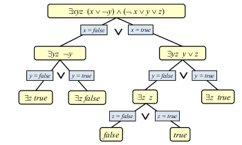
Figure 1: Example of DPLL’s search tree for the existence of satisfying assignments. We show the full tree even though the search typically stops when the first satisfying assignment is found.

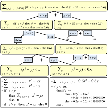
Figure 2: SGDPLL($T$) for summation with a background theory of difference arithmetic on bounded integers. Variables $x,y,z$ are in $\{1,\dots,1000\}$ but SGDPLL($T$) does not iterate over all these values. It splits the problem according to literals in the background theory, simplifying it until the sum is over a literal-free expression (here, polynomials). Splits on literals in the quantified variable $x$ split its quantifier $\sum$ and the solutions to the sub-problems are combined by $+$ (quantifier-splitting as explained in Section 4). The split on $y\neq 5$ does not involve index $x$, so it creates an if-then-else expression (if-splitting). Literal $y\neq 5$ (and its negation) does not need to be in the sub-solutions, from which it is simplified away; it will be present in the final solution only, as the if-then-else condition. When the base case with a literal-free expression is obtained, the specific theory solver computes its solution as detailed in the Appendices (lower rectangular boxes). The figure omits the simplification of the overall resulting expression by summation of sub-solutions and possible elimination of redundant literals. Problems with multiple $\sum$ quantifiers are solved by successively solving the innermost one, treating the indices of external sums as free variables.

The Davis-Putnam-Logemann-Loveland (DPLL) algorithm Davis et al. (1962) solves the satisfiability (or SAT) problem. SAT consists of determining whether a propositional formula $F$, expressed in conjunctive normal form (CNF), has a solution or not. A CNF is a conjunction ($\wedge$) of clauses where a clause is a disjunction ($\vee$) of literals. A literal is either a proposition (that is, a Boolean variable) or its negation. A solution to a CNF is an assignment of values from the set $\{\textsc{true},\textsc{false}\}$ to all propositions in $F$ such that at least one literal in each clause in $F$ is assigned to true.

• $\textnormal{DPLL}(F)$
     $F$: a formula in CNF. 1if $F$ is a boolean constant 2 return $F$ 3else $v\leftarrow$ pick a variable in $F$ 4 $\mathit{Sol}_{1}\leftarrow\mathit{DPLL}(\mathit{simplify}(F|\,\,\,\,v))$ 5 $\mathit{Sol}_{2}\leftarrow\mathit{DPLL}(\mathit{simplify}(F|\neg v))$ 6 return $\mathit{Sol}_{1}\vee\mathit{Sol}_{2}$

Algorithm 1 A version of the DPLL algorithm.

Algorithm 1 shows a simplified, non-optimized version of DPLL which operates on CNF formulas. It works by recursively trying assignments for each proposition, one at a time, simplifying the CNF, until $F$ is a constant (true or false), and combining the results with disjunction. Figure 1 shows an example of the execution of DPLL. DPLL is the basis for modern SAT solvers which improve it by adding sophisticated techniques such as unit propagation, watch literals, and clause learning Eén and Sörensson (2003); Marić (2009).

Satisfiability Modulo Theories (SMT) algorithms Barrett et al. (2009); de Moura et al. (2007); Ganzinger et al. (2004) generalize DPLL and can determine the satisfiability of a Boolean formula expressed in first-order logic, where some function and predicate symbols have specific interpretations. Examples of predicates include equalities, inequalities, and uninterpreted functions, which can then be evaluated using rules of real arithmetic. SMT algorithms condition on the literals of a background theory $T$, looking for a truth assignment to these literals that satisfies the formula. While a SAT solver is free to condition on a proposition, assigning it to either true or false regardless of previous choices (truth values of propositions are independent from each other), an SMT solver needs to also check whether a choice for one literal is consistent with the previous choices for others, according to $T$. This is done by a theory-specific model checker, provided as a parameter.

SGDPLL($T$) is, like SMT algorithms, modulo theories but further generalizes DPLL by being symbolic and quantifier-parametric (thus “Symbolic Generalized DPLL($T$)”). These three features can be observed in the problem being solved by SGDPLL($T$) in Figure 2:

$$\sum_{x\in\{1,\dots,1000\}} \quad(\mathtt{if}\,x>y\wedge y\neq 5\,\mathtt{\;then}\,x^{2}-y\,\mathtt{\;else}\,0.9)$$

$$\quad\times(\mathtt{if}\,x=z\,\mathtt{\;then}\,x\,\mathtt{\;else}\,0.6)$$

In this example, the problem being solved requires more than propositional logic theory since equality, inequality and other functions are involved. The problem’s quantifier is a summation, as opposed to DPLL and SMT’s existential quantification $\exists$. Also, the output will be symbolic in $y$ and $z$ because these variables are not being quantified, as opposed to DPLL and SMT algorithms which implicitly assume all variables to be quantified.

Before formally describing SGDPLL($T$), we will further comment on its three key generalizations.
1. Quantifier-parametric. Satisfiability can be seen as computing the value of an existentially quantified formula; the existential quantifier can be seen as an indexed form of disjunction, so we say it is based on disjunction. SGDPLL($T$) generalizes SMT algorithms by solving any quantifier $\bigoplus$ based on a commutative associative operation $\oplus$, provided that a corresponding theory-specific solver is available for base case problems, as explained later. Examples of ($\bigoplus$, $\oplus$, ) pairs are ($\forall$,$\wedge$), ($\exists$,$\vee$), ($\sum$,$+$), and ($\prod$,$\times$). Therefore SGDPLL($T$) can solve not only satisfiability (since disjunction is commutative and associative), but also validity (using the $\forall$ quantifier), sums, products, model counting, weighted model counting, maximization, among others, for propositional logic-based, and many other, theories.
2. Modulo Theories. SMT generalizes the propositions in SAT to literals in a given theory $T$, but the theory connecting these literals remains that of boolean connectives. SGDPLL($T$) takes a theory $T=(T_{\mathcal{C}},T_{\mathcal{L}})$, composed of a constraint theory $T_{\mathcal{C}}$ and an input theory $T_{\mathcal{L}}$. DPLL propositions are generalized to literals in $T_{\mathcal{C}}$ in SGDPLL($T$), whereas the boolean connectives are generalized to functions in $T_{\mathcal{L}}$. In the example above, $T_{\mathcal{C}}$ is the theory of difference arithmetic on bounded integers, whereas $T_{\mathcal{L}}$ is the theory of $+,\times$, boolean connectives and $\mathtt{if}\,\,\mathtt{\;then}\,\,\mathtt{\;else}\,$. Of the two, $T_{\mathcal{C}}$ is the crucial one, on which inference is performed, while $T_{\mathcal{L}}$ is used simply for the simplifications after conditioning, which takes time at most linear in the input expression size.
3. Symbolic. Both SAT and SMT can be seen as computing the value of an existentially quantified formula in which all variables are quantified, and which is always equivalent to either true or false. SGDPLL($T$) further generalizes SAT and SMT by accepting quantifications over any subset of the variables in its input expression (including the empty set). The non-quantified variables are free variables, and the result of the quantification will typically depend on them. Therefore, SGDPLL($T$)’s output is a symbolic expression in terms of free variables. Section 3 shows an example of a symbolic solution.

Being symbolic allows SGDPLL($T$) to conveniently solve a number of problems, including quantifier elimination and exploitation of factorization in probabilistic inference, as discussed in Section 5.

3 $T$-Problems and $T$-Solutions

SGDPLL($T$) receives a $T$-problem (or, for short, a problem) of the form

$$\bigoplus_{x:F(x,\mathbf{y})}E(x,\mathbf{y}),$$ (1)

where $x$ is an index variable quantified by $\bigoplus$ and subject to constraint $F(x,\mathbf{y})$ in $T_{\mathcal{C}}$, with possibly the presence of free variables $\mathbf{y}$, and $E(x,\mathbf{y})$ an expression in $T_{\mathcal{L}}$. $F(x,\mathbf{y})$ is a conjunction of literals in $T_{\mathcal{C}}$, that is, a conjunctive clause. An example of a problem is

$$\sum_{x:3\leq x\wedge x\leq y}\mathtt{if}\,x>4\,\mathtt{\;then}\,y\,\mathtt{\;else}\,10+z,$$

for $x,y,z$ bounded integer variables in, say, $\{1,\dots,20\}$. The index is $x$ whereas $y,z$ are free variables.

A $T$-solution (or, for short, simply a solution) to a problem is simply a quantifier-free expression in $T_{\mathcal{L}}$ equivalent to the problem. Note that solution will often contain literals and conditional expressions dependent on the free variables. For example, the problem

$$\sum_{x:1\leq x\wedge x\leq 10}\mathtt{if}\,y>2\wedge w>y\,\mathtt{\;then}\,y\,\mathtt{\;else}\,4$$

has an equivalent conditional solution

$$\mathtt{if}\,y>2\,\mathtt{\;then}\,\mathtt{if}\,w>y\,\mathtt{\;then}\,10y\,\mathtt{\;else}\,40\,\mathtt{\;else}\,40.$$

For more general problems with multiple quantifiers, we simply successively solve the innermost problem until all quantifiers have been eliminated.

4 SGDPLL($T$)

In this section we provide the details of SGDPLL($T$), described in Algorithm 2 and exemplified in Figure 2.

4.1 Solving Base Case $T$-Problems

A problem, as defined in Equation (1), is in base case if $E(x,\mathbf{y})$ contains no literals in $T_{\mathcal{C}}$.

In this paper, $T=(T_{\mathcal{C}},T_{\mathcal{L}})$ where $T_{\mathcal{L}}$ is polynomials over bounded integer variables, and $T_{\mathcal{C}}$ is difference arithmetic de Moura et al. (2007), with atoms of the form $x<y$ or $x\leq y+c$, where $c$ is an integer constant. Strict inequalities $x<y+c$ can be represented as $x\leq y+c-1$ and the negation of $x\leq y+c$ is $y\leq x-c-1$. From now on, we shorten $a\leq x\wedge x\leq b$ to $a\leq x\leq b$.

Therefore, a base case problem for this theory is of the form $\sum_{x:F(x,\mathbf{y})}P(x,\mathbf{y})$, where $x$ is the index, $\mathbf{y}$ is a tuple of free variables, $F(x,\mathbf{y})$ is a conjunction of difference arithmetic literals, and $P(x,\mathbf{y})$ is a polynomial over $x$ and $\mathbf{y}$. We show how to fully solve difference arithmetic base cases in Appendices A and B.

4.2 Solving Non-Base Case $T$-Problems

Non-base case problems (that is, those in which $E(x,\mathbf{y})$ of Equation (1) contains literals in $T_{\mathcal{C}}$) are solved by reduction to base-case ones. While base cases are solved by theory-specific solvers, the reduction from non-base case problems to base case ones is theory-independent. This is significant as it allows SGDPLL($T$) to be expanded with new theories by providing a solver only for base case problems, analogous to the way SMT solvers require theory solvers only for conjunctive clauses, as opposed to general formulas, in those theories.

The reduction mirrors DPLL, by selecting a splitter literal $L$ present in $E(x,\mathbf{y})$ to split the problem on, generating two simpler problems:

• quantifier-splitting applies when $L$ contains the index $x$. Then two sub-problems are created, one in which $L$ is added to $F(x,\mathbf{y})$, and another in which $\neg L$ is. Their solution is then combined by the quantifier’s operation ($+$ for the case of $\sum$).

  For example, consider:

  $$\sum_{x:3<x\leq 10}\mathtt{if}\,x>4\,\mathtt{\;then}\,y\,\mathtt{\;else}\,(10+z)$$

  To remove the literal from $E(x,\mathbf{y})$, we add the literal ($x>4$) and its negation ($x\leq 4$) to the constraint on $x$, yielding two base-case problems:

  $$\Bigl{(}\sum_{x:x>4\wedge 3<x\leq 10}y\Bigr{)}+\Bigl{(}\sum_{x:x\leq 4\wedge 3<x\leq 10}(10+z)\Bigr{)}.$$

• if-splitting applies when $L$ does not contain the index $x$. Then $L$ becomes the condition of an $\mathtt{if}\,\,\mathtt{\;then}\,\,\mathtt{\;else}\,$ expression and the two simpler sub-problems are its then and else clauses.

  For example, consider

  $$\sum_{x:3<x\leq 10}\mathtt{if}\,y>4\,\mathtt{\;then}\,y\,\mathtt{\;else}\,10.$$

  Splitting on $y>4$ reduces the problem to

  $$\mathtt{if}\,y>4\,\mathtt{\;then}\,\sum_{x:3<x\leq 10}y\,\mathtt{\;else}\,\sum_{x:3<x\leq 10}10,$$

  containing two base-case problems.

The algorithm terminates because each splitting generates sub-problems with one less literal in $E(x,\mathbf{y})$, eventually obtaining base case problems. It is sound because each transformation results in an expression equivalent to the previous one.

To be a valid parameter for SGDPLL($T$), a $(T,\oplus)$-solver $S_{T}$ for theory $T=(T_{\mathcal{L}},T_{\mathcal{C}})$ must, given a problem $\bigoplus_{x:F(x,\mathbf{y})}E(x,\mathbf{y})$, recognize whether it is in base form and, if so, provide a solution $base_{T}(\bigoplus_{x:F(x,\mathbf{y})}E(x,\mathbf{y}))$.

The algorithm is presented as Algorithm 2. Note that it does not depend on difference arithmetic theory, but can use a solver for any theory satisfying the requirements above.

If the $(T,\oplus)$-solver implements the operations above in constant time in the domain size (the size of their types), then it follows that SGDPLL($T$) will have complexity independent of the domain size. This is the case for the solver for difference arithmetic and will typically be the case for many other solvers.

Algorithm 2 Symbolic Generalized DPLL (SGDPLL($T$)),   omitting pruning, heuristics and optimizations.

• $\textnormal{SGDPLL($T$)}(\bigoplus_{x:F(x,\mathbf{y})}E(x,\mathbf{y}))$
      Returns a $T$-solution for $\bigoplus_{x:F(x,\mathbf{y})}E(x,\mathbf{y})$. 1if $E(x,\mathbf{y})$ is literal-free (base case) 2 return $base_{T}(\bigoplus_{x:F(x,\mathbf{y})}E(x,\mathbf{y}))$ 3else 4 $L\leftarrow$ a literal in $E(x,\mathbf{y})$ 5 $E^{\prime}\;\leftarrow E$ with $L$ replaced by true and simplified 6 $E^{\prime\prime}\leftarrow E$ with $L$ replaced by false and simplified 7 if $L$ contains index $x$ 8 $\mathit{Sub}_{1}\leftarrow\bigoplus_{x:F(x,\mathbf{y})\wedge L}\;\;E^{\prime}$ 9 $\mathit{Sub}_{2}\leftarrow\bigoplus_{x:F(x,\mathbf{y})\wedge\neg L}E^{\prime\prime}$ 10 else // $L$ does not contain index $x$: 11 $\mathit{Sub}_{1}\leftarrow\bigoplus_{x:F(x,\mathbf{y})}\;E^{\prime}$ 12 $\mathit{Sub}_{2}\leftarrow\bigoplus_{x:F(x,\mathbf{y})}\;E^{\prime\prime}$ 13 $S_{1}\leftarrow\text{SGDPLL($T$)}(Sub_{1})$ 14 $S_{2}\leftarrow\text{SGDPLL($T$)}(Sub_{2})$ 15 if $L$ contains index $x$ 16 return $S_{1}\oplus S_{2}$ 17 else return the expression $\mathtt{if}\,L\,\mathtt{\;then}\,S_{1}\,\mathtt{\;else}\,S_{2}$

4.3 Optimizations

In the simple form presented above, SGDPLL($T$) may generate solutions such as $\mathtt{if}\,x=3\,\mathtt{\;then}\,\mathtt{if}\,x\neq 4\,\mathtt{\;then}\,y\,\mathtt{\;else}\,z\,\mathtt{\;else}\,w$ in which literals are implied (or negated) by the context they are in, and are therefore redundant. Redundant literals can be eliminated by keeping a conjunction of all choices (sides of literal splittings) made at any given point (the context) and using any SMT solver to incrementally decide when a literal or its negation is implied, thus pruning the search as soon as possible. Note that a $(T,\oplus)$-solver for SGDPLL($T$) appropriate for $\exists$ can be used for this, although here there is the opportunity to leverage the very efficient SMT systems already available.

Modern SAT solvers benefit enormously from unit propagation, watched literals and clause learning Eén and Sörensson (2003); Marić (2009). In DPLL, unit propagation is performed when all but one literal $L$ in a clause are assigned false. For this unit clause, and as a consequence, for the CNF problem, to be satisfied, $L$ must be true and is therefore immediately assigned that value wherever it occurs, without the need to split on it. Detecting unit clauses, however, is expensive if performed by naively checking all clauses at every splitting. Watched literals is a data structure scheme that allows only a small portion of the literals to be checked instead. Clause learning is based on detecting a subset of jointly unsatisfiable literals when the splits made so far lead to a contradiction, and keeping it for detecting contradictions sooner as the search goes on. In the SGDPLL($T$) setting, unit propagation, watched literals and clause learning can be generalized to its not-necessarily-Boolean expressions; we leave this presentation for future work.

5 Probabilistic Inference Modulo Theories

Let $P(X_{1}=x_{1},\dots,X_{n}=x_{n})$ be the joint probability distribution on random variables $\{X_{1},\dots,X_{n}\}$. For any tuple of indices $t$, we define $X_{t}$ to be the tuple of variables indexed by the indices in $t$, and abbreviate the assignments $(X=x)$ and $(X_{t}=x_{t})$ by simply $x$ and $x_{t}$, respectively. Let $\bar{t}$ be the tuple of indices in $\{1,\dots,n\}$ but not in $t$.

The marginal probability distribution of a subset of variables $X_{q}$ is one of the most basic tasks in probabilistic inference, defined as

$$P(x_{q})=\sum_{x_{\bar{q}}}P(x)$$

which is a summation on a subset of variables occurring in an input expression, and therefore solvable by SGDPLL($T$).

If $P(x)$ is expressed in the language of input and constraint theories appropriate for SGDPLL($T$) (such as the one shown in Figure 2), then it can be solved by SGDPLL($T$), without first converting its representation to a much larger one based on tables. The output will be a summation-free expression in the assignment variables $x_{q}$ representing the marginal probability distribution of $X_{q}$.

Let us show how to represent $P(x)$ with an expression in $T_{\mathcal{L}}$ through an example. Consider a hypothetical generative model involving random variables with bounded integer values and describing the influence of variables such as the number of terror attacks, the Dow Jones index and newly created jobs on the number of people who like an incumbent and an challenger politicians:

$$\mathit{attacks}\sim\mathit{Uniform}(0..20)$$

$$\mathit{newJobs}\sim\mathit{Uniform}(0..100000)$$

$$\mathit{dow}\sim\mathit{Uniform}(11000..18000)$$

$$\mathit{likeChallenger}\sim\mathit{Uniform}(0..N)$$

$$P(\mathit{likeIncumbent}\in 0..N|\mathit{dow},\mathit{newJobs},\mathit{attacks})$$

$$=\begin{cases}\frac{0.4}{\lfloor 0.7N\rfloor}\text{, if }\mathit{dow}>16000\wedge\mathit{newJobs}>70000)\\ \qquad\qquad\wedge\;\mathit{likeIncumbent}<\lfloor 0.7N\rfloor\\ \frac{0.6}{N+1-\lfloor 0.7N\rfloor}\text{, if }\mathit{dow}>16000\wedge\mathit{newJobs}>70000)\\ \qquad\qquad\quad\quad\;\;\wedge\;\mathit{likeIncumbent}\geq\lfloor 0.7N\rfloor\\ \frac{0.8}{\lfloor 0.5N\rfloor}\text{, if }\mathit{dow}<13000\wedge\mathit{newJobs}<30000)\\ \qquad\qquad\wedge\;\mathit{likeIncumbent}<\lfloor 0.5N\rfloor\\ \frac{0.2}{N+1-\lfloor 0.5N\rfloor}\text{, if }\mathit{dow}<13000\wedge\mathit{newJobs}<30000)\\ \qquad\qquad\qquad\wedge\;\mathit{likeIncumbent}\geq\lfloor 0.5N\rfloor\\ \frac{0.9}{\lfloor 0.6N\rfloor}\text{, none of the above and }(\mathit{attacks}\leq 4)\\ \qquad\qquad\wedge\;\mathit{likeIncumbent}<\lfloor 0.6N\rfloor\\ \frac{0.1}{N+1-\lfloor 0.6N\rfloor}\text{, none of the above and }(\mathit{attacks}\leq 4)\\ \qquad\qquad\qquad\wedge\;\mathit{likeIncumbent}\geq\lfloor 0.6N\rfloor\\ \frac{1}{N+1}\text{, otherwise }\end{cases}$$

which indicates that, if the Dow Jones index is above 16000 or there were more than 70000 new jobs, then there is a $0.4$ probability that the number of people who like the incumbent politician is below around 70% of $N$ people (and that probability is uniformly distributed among those $\lfloor 0.7N\rfloor$ values), with the remaining $0.6$ probability mass uniformly distributed over the remaining $N+1-\lfloor 0.7N\rfloor$ values. Similar distributions hold for other conditions. Note that $N$ is a known parameter and the actual representation will contain the evaluations of its expressions. For example, for $N=10^{8}$, $0.8/\lfloor 0.5N\rfloor$ is replaced by $1.6\times 10^{-8}$.

The joint probability distribution

$$P(\mathit{attacks},\mathit{newJobs},\mathit{dow},\mathit{likeChallenger},\mathit{likeIncumbent})$$

is simply the product of $P(\mathit{attacks})$, $P(\mathit{newJobs})$ and so on. $P(\mathit{attacks})$ can be expressed by

$$\mathtt{if}\,\,\mathit{attacks}\geq 0\wedge\mathit{attacks}\leq 20\,\mathtt{\;then}\,1/21\,\mathtt{\;else}\,0$$

because of its distribution $\mathit{Uniform}(0..20)$, and the other uniform distributions are represented analogously. $P(\mathit{likeIncumbent}|\mathit{dow},\mathit{newJobs},\mathit{attacks})$ is represented by the expression

$$\mathtt{if}\;{\mathit{dow}>16000\wedge\mathit{newJobs}>70000}$$

$$\quad\;\mathtt{then}\;{\mathtt{if}\;{\mathit{likeIncumbent}<\lfloor 0.7N\rfloor}}$$

$$\quad\quad\;\mathtt{then}\;{{\frac{0.4}{\lfloor 0.7N\rfloor}}}$$

$$\quad\quad\;\mathtt{else}\;{{\frac{0.6}{N+1-\lfloor 0.7N\rfloor}}}$$

$$\quad\;\mathtt{else}\;{\mathtt{if}\;{\mathit{dow}<13000\wedge\mathit{newJobs}<30000}\;{\dots}}$$

again noting that $N$ is fixed and the actual expression contains the constants computed from $\lfloor 0.7N\rfloor$, $\frac{0.4}{\lfloor 0.7N\rfloor}$, and so on.

Other probabilistic inference problems can be also solved by SGDPLL($T$). Belief updating consists of computing the posterior probability of $X_{q}$ given evidence on $X_{e}$, which is defined as

$$P(x_{q}|x_{e})=\frac{P(x_{q},x_{e})}{P(x_{e})}=\frac{P(x_{q},x_{e})}{\sum_{x_{q}}P(x_{q},x_{e})}$$

which can be computed with two applications of SGDPLL($T$): first, we obtain a summation-free expression $S$ for $P(x_{q},x_{e})$, which is $\sum_{x_{\mkern 1.5mu\overline{\mkern-1.5mu(q,e)\mkern-1.5mu}\mkern 1.5mu}}P(x)$, and then again $S$ for $\sum_{x_{q}}P(x_{q},x_{e})$, which is $\sum_{x_{q}}S$.

We can also use SGDPLL($T$) to compute the most likely assignment on $X_{q}$, defined by $\max_{x_{q}}P(x)$, since $\max$ is a commutative and associative operation.

Applying SGDPLL($T$) in the manner above does not take advantage of factorized representations of joint probability distributions, a crucial aspect of efficient probabilistic inference. However, it can be used as a basis for an algorithm, Symbolic Generalized Variable Elimination Modulo Theories (SGVE($T$)), analogous to Variable Elimination (VE) Zhang and Poole (1994); Dechter (1999) for graphical models, that exploits factorization. SGVE($T$) works in the exact same way VE does, but using SGDPLL($T$) whenever VE uses marginalization over a table. Note that SGDPLL($T$)’s symbolic treatment of free variables is crucial for the exploitation of factorization, since typically only a subset of variables is eliminated at each step. Also note that SGVE($T$), like VE, requires the additive and multiplicative operations to form a c-semiring Bistarelli et al. (1997).

Finally, because of SGDPLL($T$) and SGVE($T$) symbolic capabilities, it is also possible to compute symbolic query results as functions of uninstantiated evidence variables, without the need to iterate over all their possible values. For the election example above with $N=10^{8}$, we can compute $P(\mathit{likeIncumbent}>\mathit{likeChallenger}|\mathit{newJobs})$ without providing a value for $\mathit{newJobs}$, obtaining the symbolic result

$$\mathtt{if}\;{\mathit{newJobs}>70000}$$

$$\quad\;\mathtt{then}\;{0.5173}$$

$$\quad\;\mathtt{else}\;{\mathtt{if}\;{\mathit{newJobs}<30000}}$$

$$\quad\qquad\qquad\;\mathtt{then}\;{0.4316}$$

$$\quad\qquad\qquad\;\mathtt{else}\;{0.4642}$$

without iterating over all values of $\mathit{newJobs}$. This result can be seen as a compiled form to be used when the value of $\mathit{newJob}$ is known, without the need to reprocess the entire model.

6 Experiment

We conduct a proof-of-concept experiment comparing our implementation of SGDPLL($T$)-based SGVE($T$) (available from the corresponding author’s web page) to the state-of-the-art probabilistic inference solver variable elimination and conditioning (VEC) Gogate and Dechter (2011), on the election example described above. The model is simple enough for SGVE($T$) to solve the query $P(\mathit{likeIncumbent}>\mathit{likeChallenger}|\mathit{newJobs}=80000\wedge\mathit{dow}=17000)$ exactly in around 2 seconds on a desktop computer with an Intel E5-2630 processor, which results in $0.6499$ for $N=10^{8}$. The run time of SGVE($T$) is constant in $N$; however, the number of values is too large for a regular solver such as VEC to solve exactly, because the tables involved will be too large even to instantiate. By decreasing the range of $\mathit{newJobs}$ to $0..100$, of $\mathit{dow}$ to $110..180$ and $N$ to just $500$, we managed to use VEC but it still takes $51$ seconds to solve the problem.

7 Related work

SGDPLL($T$) is related to many different topics in both logic and probabilistic inference literature, besides the strong links to SAT and SMT solvers.

SGDPLL($T$) is a lifted inference algorithm Poole (2003); de Salvo Braz (2007); Gogate and Domingos (2011), but lifted algorithms so far have concerned themselves only with relational formulas with equality. We have not yet developed the theory solvers for relational representations required for SGDPLL($T$) to do the same, but we intend to do so using the already developed modulo-theories mechanism available. On the other hand, we have presented probabilistic inference over difference arithmetic for the first time in the lifted inference literature.

Sanner and Abbasnejad (2012) presents a symbolic variable elimination algorithm (SVE) for hybrid graphical models described by piecewise polynomials. SGDPLL($T$) is similar, but explicitly separates the generic and theory-specific levels, and mirrors the structure of DPLL and SMT. Moreover, SVE operates on Extended Algebraic Decision Diagrams (XADDs), while SGDPLL($T$) operates directly on arbitrary expressions formed with the operators in $T_{\mathcal{L}}$ and $T_{\mathcal{C}}$. Finally, in this paper we present a theory solver for sums over bounded integers, while that paper describes an integration solver for continuous numeric variables (which can be adapted as an extra theory solver for SGDPLL($T$)). Belle et al. (2015a, b) extends Sanner and Abbasnejad (2012) by also adopting DPLL-style splitting on literals, allowing them to operate directly on general boolean formulas, and by focusing on the use of a SMT solver to prune away unsatisfiable branches. However, it does not discuss the symbolic treatment of free variables and its role in factorization, and does not focus on the generic level (modulo theories) of the algorithm.

SGDPLL($T$) generalizes several algorithms that operate on mixed networks Mateescu and Dechter (2008) – a framework that combines Bayesian networks with constraint networks, but with a much richer representation. By operating on richer languages, SGDPLL($T$) also generalizes exact model counting approaches such as RELSAT Bayardo, Jr. and Pehoushek (2000) and Cachet Sang et al. (2005), as well as weighted model counting algorithms such as ACE Chavira and Darwiche (2008) and formula-based inference Gogate and Domingos (2010), which use the CNF and weighted CNF representations respectively.

8 Conclusion and Future Work

We have presented SGDPLL($T$) and its derivation SGVE($T$), algorithms formally able to solve a variety of problems, including probabilistic inference modulo theories, that is, capable of being extended with solvers for richer representations than propositional logic, in a lifted and exact manner.

Future work includes additional theories and solvers of interest, mainly among them algebraic data types and uninterpreted relations; modern SAT solver optimization techniques such as watched literals, unit propagation and clause learning, and anytime approximation schemes that offer guaranteed bounds on approximations that converge to the exact solution.

Appendix A Solver for Sum and Difference Arithmetic

This appendix describes a $T$-solver for the base case $T$-problem $\sum_{x:F(x,\mathbf{y})}P(x,\mathbf{y})$ for $T=(T_{\mathcal{C}},T_{\mathcal{L}})$ where $T_{\mathcal{C}}$ is difference arithmetic and $T_{\mathcal{L}}$ is the language of polynomials, $x$ is a variable and $\mathbf{y}$ is a tuple of free variables. Because this is a base case, $P(x,\mathbf{y})$ is a polynomial and contains no literals. $F(x,\mathbf{y})$ is a conjunctive clause of difference arithmetic literals.

The solver also receives, as an extra input, a conjunctive clause $C(\mathbf{y})$ (a context) on free variables only, and its output is a quantifier-free $T$-solution $S(\mathbf{y})$ such that $C(\mathbf{y})\Rightarrow S(\mathbf{y})=\sum_{x:F(x,\mathbf{y})}P(x,\mathbf{y})$. In other words, $C(\mathbf{y})$ encodes the assignments to $\mathbf{y}$ of interest in a given context, and the solution needs to be equal to the problem only when $\mathbf{y}$ satisfies $C(\mathbf{y})$. The context starts with true but is set to more restrictive formulas in the solver’s recursive calls.

We assume an SMT (Satisfiability Modulo Theory) solver that can decide whether a conjunctive clause in the background theory (here, difference arithmetic) is satisfiable or not.

The intuition behind the solver is gradually removing ambiguities until we are left with a single lower bound, a single upper bound, and unique disequalities on index $x$. For example, if the index $x$ has two lower bounds (two literals $x>y$ and $x>z$), then we split on $y>z$ to decide which lower bound implies the other, eliminating it. Likewise, if there are two literals $x\neq y$ and $x\neq z$, we split on $y=z$, either eliminating the second one if this is true, or obtaining a uniqueness guarantee otherwise. Once we have a single lower bound, single upper bound and unique disequalities, we can solve the problem more directly, as detailed in Case 8 below.

Let $\mathit{Sum}(x,F(x,\mathbf{y}),P(x,\mathbf{y}),C(\mathbf{y}))$ be the result of invoking the solver its inputs, and $\alpha$, $\beta$ stand for any expression. The following cases are applied in order:

Case 0

if $C(\mathbf{y})$ is unsatisfiable, return any expression (say, $0$).

Case 1

if any literals in $F(x,\mathbf{y})$ are trivially contradictory, such as $\alpha\neq\alpha$, $\alpha<\alpha$, $\alpha\neq\beta$ for $\alpha$ and $\beta$ two distinct constants, return $0$.

Case 2

if any literals in $F(x,\mathbf{y})$ are trivially true, (such as $\alpha=\alpha$ or $\alpha\geq\alpha$), or are redundant due to being identical to a previous literal, return $\mathit{Sum}(x,F^{\prime}(x,\mathbf{y}),P(x,\mathbf{y}),C(\mathbf{y}))$, for $F^{\prime}(x,\mathbf{y})$ equal to $F(x,\mathbf{y})$ after removing such literals.

Case 3

if $F(x,\mathbf{y})$ contains literal $x=\alpha$, return $\mathit{Sum}(x,F^{\prime}(x,\mathbf{y}),P(x,\mathbf{y}),C(\mathbf{y}))$, for $F^{\prime}(x,\mathbf{y})$ equal to $F(x,\mathbf{y})$ after replacing every other occurrence of $x$ with $\alpha$.

Case 4

if any literal $L$ in $F(x,\mathbf{y})$ does not involve $x$, return the expression

$$\mathtt{if}\,L\,\mathtt{\;then}\,\mathit{Sum}(x,F^{\prime}(x,\mathbf{y}),P(x,\mathbf{y}),C(\mathbf{y})\wedge L)\,\mathtt{\;else}\,0,$$

for $F^{\prime}(x,\mathbf{y})$ equal to $F(x,\mathbf{y})$ after removing $L$.

Case 5

if $F(x,\mathbf{y})$ contains only literal $x=\alpha$, return $P(\alpha,\mathbf{y})$.

Case 6

if $F(x,\mathbf{y})$ contains literals $x\geq\alpha$ or $x<\beta$, return $\mathit{Sum}(x,F^{\prime}(x,\mathbf{y}),P(x,\mathbf{y}),C(\mathbf{y}))$, for $F^{\prime}(x,\mathbf{y})$ equal to $F(x,\mathbf{y})$ after replacing such literals by $x>\alpha-1$ and $x\leq\beta+1$, respectively. This guarantees that all lower bounds for $x$ are strict, and all upper bounds are non-strict.

Case 7

if $F(x,\mathbf{y})$ contains literal $x>\alpha$ ($\alpha$ is a strict lower bound), and literal $x>\beta$ or literal $x\neq\beta$, let literal $L$ be $\alpha<\beta$. Otherwise, if $F(x,\mathbf{y})$ contains literal $x\leq\alpha$ ($\alpha$ is a non-strict upper bound), and literal $x\geq\beta$ or literal $x\neq\beta$, let literal $L$ be $\beta\leq\alpha$. Otherwise, if $F(x,\mathbf{y})$ contains literal $x\neq\alpha$ and literal $x\neq\beta$, let $L$ be $\alpha=\beta$. Otherwise, if $F(x,\mathbf{y})$ contains literal $x>\alpha$ and literal $x\leq\beta$, let $L$ be $\alpha<\beta$. Then, if $C(\mathbf{y})\wedge L$ and $C(\mathbf{y})\wedge\neg L$ are both satisfiable (that is, $C(\mathbf{y})$ does not imply $\alpha=\beta$ either way), return the expression

$$\mathtt{if}\;{L}\;\mathtt{then}\;{\mathit{Sum}(x,F(x,\mathbf{y}),P(x,\mathbf{y}),C(\mathbf{y})\wedge L)}$$

$$\qquad\;\mathtt{else}\;{\mathit{Sum}(x,F(x,\mathbf{y}),P(x,\mathbf{y}),C(\mathbf{y})\wedge\neg L)}.$$

Case 8

At this point, $F(x,\mathbf{y})$ and $C(\mathbf{y})$ jointly define a single strict lower bound $l$ and non-strict upper bound $u$ for $x$, and $\{\beta_{1},\dots,\beta_{k}\}$ such that $x\neq\beta_{i}$ and $l<\beta_{i}\leq u$ for every $i\in\{1,\dots,k\}$. If $C(\mathbf{y})$ implies $u-l<k$, return $0$. Otherwise, return $\mathit{FH}\bigl{(}\sum_{x:l<x\leq u}P(x,\mathbf{y})\bigr{)}-P(\beta_{1},\mathbf{y})-\dots-P(\beta_{k},\mathbf{y})$, where $\mathit{FH}$ is an extended version of Faulhaber’s formula Knuth (1993). The extension is presented in Appendix B and only involves simple algebraic manipulation. The fact that Faulhaber’s formula can be used in time independent of $u-l$ renders the solver complexity independent of the index’s domain size.

Theorem A.1

Given $x$, $F(x,\mathbf{y})$, $P(x,\mathbf{y})$, $C(\mathbf{y})$, the solver computes $\mathit{Sum}(x,F(x,\mathbf{y}),P(x,\mathbf{y}),C(\mathbf{y}))$ in time independent of the domain sizes of $x$ and $\mathbf{y}$, and

$$\forall\mathbf{y}\;C(\mathbf{y})\Rightarrow\\ \mathit{Sum}(x,F(x,\mathbf{y}),P(x,\mathbf{y}),C(\mathbf{y}))\;=\sum_{x:F(x,\mathbf{y})}P(x,\mathbf{y}).$$

Proof.

(Sketch) Cases 0-2 are trivial (Case 0, in particular, is based on the fact that any solution is correct if $C(\mathbf{y})$ is false).

Cases 3 and 4 cover cases in which $x$ is bounded to a value and successively eliminate all other literals until trivial Case 5 applies. The left lower box of Figure 2 exemplifies this pattern.

Case 6 and 7 gradually determine a single strict lower bound $l$ and non-strict upper bound $u$ for $x$, determine that $l<u$, as well as which expressions $\beta_{i}$ constrained to be distinct from $x$ are within $l$ and $u$, and are distinct from each other. This provides the necessary information for Case 8 to use Faulhaber’s formula and determine a solution. The right lower box of Figure 2 exemplifies this pattern. ∎

Appendix B Computing Faulhaber’s extension $\mathit{FH}$

We now proceed to explain how $FH$ can computed the sum

$$\sum_{x:l<x\leq u}t_{0}+t_{1}x+\dots+t_{n}x^{n}$$

where $x$ is an integer index and $t_{i}$ are monomials, possibly including numeric constants and powers of free variables.

Faulhaber’s formula Knuth (1993) solves the simpler sum of powers problem $\sum_{k=1}^{n}k^{p}$:

$$\sum_{k=1}^{n}k^{p}={\frac{1}{p+1}}\sum_{j=0}^{p}(-1)^{j}{p+1\choose j}B_{j}n^{p+1-j},$$

where $B_{j}$ is a Bernoulli number defined as

$$B_{j} =1-\sum_{k=0}^{j-1}\binom{j}{k}\frac{B_{k}}{j-k+1}$$

$$B_{0} =1.$$

The original problem can be reduced to a sum of powers in the following manner, where $t,r,s,v,w$ are families of monomials (possibly including numeric constants) in the free variables:

$$\sum_{x:l<x\leq u}t_{0}+t_{1}x+\dots+t_{n}x^{n}$$

$$=\sum_{i=0}^{n}\quad\sum_{x:l<x\leq u}t_{i}x^{i}$$

$$=\sum_{i=0}^{n}\sum_{x=1}^{u-l}t_{i}(x+l)^{i}$$

$$=\sum_{i=0}^{n}\sum_{x=1}^{u-l}t_{i}\sum_{q=0}^{i}r_{q}x^{q}\quad\text{(by expanding the binomial)}$$

$$=\sum_{i=0}^{n}\sum_{x=1}^{u-l}\sum_{q=0}^{i}t_{i}r_{q}x^{q}$$

$$=\sum_{i=0}^{n}\sum_{q=0}^{i}t_{i}r_{q}\sum_{x=1}^{u-l}x^{q}\;\text{(inverting sums to apply Faulhaber's)}$$

$$=\sum_{i=0}^{n}\sum_{q=0}^{i}{t_{i}r_{q}\over q+1}\sum_{j=0}^{q}(-1)^{j}{q+1\choose j}B_{j}(u-l)^{q+1-j}$$

$$=\sum_{i=0}^{n}\sum_{q=0}^{i}\sum_{j=0}^{q}s_{i,q,j}(u-l)^{q+1-j}$$

$$=\sum_{i=0}^{n}\sum_{q=0}^{i}\sum_{j=0}^{q}s_{i,q,j}\sum_{l=1}^{q+1}v_{l}\quad\text{(by expanding the binomial)}$$

$$=\sum_{i=0}^{n}\sum_{q=0}^{i}\sum_{j=0}^{q}\sum_{l=1}^{q+1}s_{i,q,j}v_{l}$$

$$=w_{0}+w_{1}+\dots+w_{n^{\prime}}\quad\text{(since $n$ is a known constant)}$$

where $n^{\prime}$ is function of $n$ in $O(n^{4})$ (the time complexity for computing Bernoulli numbers up to $B_{n}$ is in $O(n^{2})$).

Because the time and space complexity of the above computation depends on the initial degree $n$ and the degrees of free variables in the monomials, it is important to understand how these degrees are affected. Let $d_{l}$ be the initial degree of the variable present in $l$ in $t$ monomials. Its degree is up to $n$ in $r$ monomials (because of the binomial expansion with $i$ being up to $n$), and thus up to $d_{l}+n$ in $s$ monomials (because of the multiplication of $t_{i}$ and $r_{q}$). The variable has degree up to $n+1$ in monomials $v$, with degree up to $d_{l}+2n+1$ in the final polynomial. The variable in $u$ keeps its initial degree $d_{u}$ until it is increased by up to $n+1$ in $v$, with final degree up to $d_{u}+n+1$. The remaining variables keep their original degrees. This means that degrees grow only linearly over multiple applications of the above. This combines with the $O(n^{4})$ per-step complexity to a $O(n^{5})$ overall complexity for $n$ the maximum initial degree for any variable. Note how this time complexity is constant in $x$’s domain size.

References

- Afshar et al. [2016] Hadi Mohasel Afshar, Scott Sanner, and Christfried Webers. Closed-form gibbs sampling for graphical models with algebraic constraints. In Dale Schuurmans and Michael P. Wellman, editors, AAAI, pages 3287–3293. AAAI Press, 2016.
- Barrett et al. [2009] C. W. Barrett, R. Sebastiani, S. A. Seshia, and C. Tinelli. Satisfiability Modulo Theories. In Armin Biere, Marijn Heule, Hans van Maaren, and Toby Walsh, editors, Handbook of Satisfiability, volume 185 of Frontiers in Artificial Intelligence and Applications, pages 825–885. IOS Press, 2009.
- Bayardo, Jr. and Pehoushek [2000] R. J. Bayardo, Jr. and J. D. Pehoushek. Counting Models Using Connected Components. In Proceedings of the Seventeenth National Conference on Artificial Intelligence, pages 157–162, Austin, TX, 2000. AAAI Press.
- Belle et al. [2015a] Vaishak Belle, Andrea Passerini, and Guy Van den Broeck. Probabilistic inference in hybrid domains by weighted model integration. In Proceedings of 24th International Joint Conference on Artificial Intelligence (IJCAI), 2015.
- Belle et al. [2015b] Vaishak Belle, Guy Van den Broeck, and Andrea Passerini. Hashing-based approximate probabilistic inference in hybrid domains. In Proceedings of the 31st Conference on Uncertainty in Artificial Intelligence (UAI), 2015.
- Bistarelli et al. [1997] Stefano Bistarelli, Ugo Montanari, and Francesca Rossi. Semiring-based constraint satisfaction and optimization. J. ACM, 44(2):201–236, March 1997.
- Chavira and Darwiche [2008] M. Chavira and A. Darwiche. On probabilistic inference by weighted model counting. Artificial Intelligence, 172(6-7):772–799, 2008.
- Davis et al. [1962] M. Davis, G. Logemann, and D. Loveland. A machine program for theorem proving. Communications of the ACM, 5:394–397, 1962.
- de Moura et al. [2007] Leonardo de Moura, Bruno Dutertre, and Natarajan Shankar. A tutorial on satisfiability modulo theories. In Computer Aided Verification, 19th International Conference, CAV 2007, Berlin, Germany, July 3-7, 2007, Proceedings, volume 4590 of Lecture Notes in Computer Science, pages 20–36. Springer, 2007.
- de Salvo Braz et al. [2016] R. de Salvo Braz, C. O’Reilly, V. Gogate, and V. Dechter. Probabilistic Inference Modulo Theories. In Proceedings of the Twenty-Fifth International Joint Conference on Artificial Intelligence, New York, USA, 2016.
- de Salvo Braz [2007] R. de Salvo Braz. Lifted First-Order Probabilistic Inference. PhD thesis, University of Illinois, Urbana-Champaign, IL, 2007.
- Dechter [1999] R. Dechter. Bucket elimination: A unifying framework for reasoning. Artificial Intelligence, 113:41–85, 1999.
- Eén and Sörensson [2003] N. Eén and N. Sörensson. An Extensible SAT-solver. In SAT Competition 2003, volume 2919 of Lecture Notes in Computer Science, pages 502–518. Springer, 2003.
- Ganzinger et al. [2004] Harald Ganzinger, George Hagen, Robert Nieuwenhuis, Albert Oliveras, and Cesare Tinelli. DPLL( T): Fast Decision Procedures. 2004.
- Getoor and Taskar [2007] L. Getoor and B. Taskar, editors. Introduction to Statistical Relational Learning. MIT Press, 2007.
- Gogate and Dechter [2011] V. Gogate and R. Dechter. SampleSearch: Importance sampling in presence of determinism. Artificial Intelligence, 175(2):694–729, 2011.
- Gogate and Domingos [2010] V. Gogate and P. Domingos. Formula-Based Probabilistic Inference. In Proceedings of the Twenty-Sixth Conference on Uncertainty in Artificial Intelligence, pages 210–219, 2010.
- Gogate and Domingos [2011] V. Gogate and P. Domingos. Probabilistic Theorem Proving. In Proceedings of the Twenty-Seventh Conference on Uncertainty in Artificial Intelligence, pages 256–265. AUAI Press, 2011.
- Goodman et al. [2012] Noah D. Goodman, Vikash K. Mansinghka, Daniel M. Roy, Keith Bonawitz, and Daniel Tarlow. Church: a language for generative models. CoRR, abs/1206.3255, 2012.
- Knuth [1993] Donald E. Knuth. Johann Faulhaber and Sums of Powers. Mathematics of Computation, 61(203):277–294, 1993.
- Marić [2009] Filip Marić. Formalization and implementation of modern sat solvers. Journal of Automated Reasoning, 43(1):81–119, 2009.
- Mateescu and Dechter [2008] R. Mateescu and R. Dechter. Mixed deterministic and probabilistic networks. Annals of Mathematics and Artificial Intelligence, 54(1-3):3–51, 2008.
- Poole [2003] D. Poole. First-Order Probabilistic Inference. In Proceedings of the Eighteenth International Joint Conference on Artificial Intelligence, pages 985–991, Acapulco, Mexico, 2003. Morgan Kaufmann.
- Sang et al. [2005] T. Sang, P. Beame, and H. A. Kautz. Heuristics for Fast Exact Model Counting. In Eighth International Conference on Theory and Applications of Satisfiability Testing, pages 226–240, 2005.