Benign-Malignant Lung Nodule Classification with Geometric and Appearance Histogram Features

Abstract

Lung cancer accounts for the highest number of cancer deaths globally. Early diagnosis of lung nodules is very important to reduce the mortality rate of patients by improving the diagnosis and treatment of lung cancer. This work proposes an automated system to classify lung nodules as malignant and benign in CT images. It presents extensive experimental results using a combination of geometric and histogram lung nodule image features and different linear and non-linear discriminant classifiers. The proposed approach is experimentally validated on the LIDC-IDRI public lung cancer screening thoracic computed tomography (CT) dataset containing nodule level diagnostic data. The obtained results are very encouraging correctly classifying $82\%$ of malignant and $93\%$ of benign nodules on unseen test data at best.

I INTRODUCTION

Uncontrolled abnormal cell growth in any part of the body leads to space occupation which might be a cancer. When these abnormal cells are growing in the lung area they might lead to lung cancer. Lung cancer accounted for $19.5\%$ of the total cancer related deaths in 2012 – the highest number of all cancer related deaths globally [8]. Lung cancer appears as pulmonary nodules which are small round or oval-shaped growth in the lung. But, all pulmonary nodules are not cancerous and in fact over $90\%$ of pulmonary nodules that are smaller than two centimeters in diameter are benign complicating proper diagnosis.

The main problem with lung cancer is that the majority of patients have evidence of spread at the time of presentation [14]. But, early diagnosis can improve the effectiveness of treatment and increase the patient’s chance of survival; hence, early detection through screening is of vital importance. Of the utilized imaging modalities to screen for lung cancer, it has recently been shown that Computed Tomography (CT) screening does actually lead to reduced deaths from lung cancer [1]. Consequently, radiologists will have to screen several scans on a daily basis. This puts increased burden which could lead to mistakes due to the overwhelming number of cases handled. To alleviate this burden, Computer Aided Diagnosis (CADx) systems can be used to help radiologists in terms of both accuracy and speed. Some studies have indeed shown improvements in radiologist’s performance through the use of CAD systems, e.g., [16]. In line with this, this work investigates image processing and machine learning techniques for automated lung nodule benign and malignant classification.

This work focuses on benign and malignant nodule classification, primarily for two reasons: (i) it is the least investigated category in the literature [7], and (ii) it has been recently getting more attention to a point that there are grand challenges organized on it [4]. Since the malignancy of lung nodules correlates highly with their geometrical size, shape, and appearance, this work proposes to investigate pattern recognition and machine learning techniques to automatically classify benign and malignant nodules based on these features. Specifically, the study focuses on evaluation of different linear and non-linear discriminant classifiers extensively used in the machine learning and pattern recognition domains – namely: logistic regression, linear Support Vector Machines (SVM), K-nearest neighbors (K-NN), discrete AdaBoost, and random forest – with a heterogeneous feature set componsed of geometric, gray scale histogram, and oriented gradient histogram features extracted from CT images. The proposed approach is experimentally validated on the LIDC-IDRI public lung cancer screening thoracic computed tomography (CT) dataset containing nodule level diagnostic data. The obtained results are very encouraging, correctly classifying $82\%$ of malignant and $93\%$ of benign nodules on unseen test data at best.

I-A Related Work

The main approach utilized in the literature for lung nodule classification follows a two step approach which uses a feature extraction and classification steps [10, 12]. In these approaches, the classifiers are trained using labeled dataset in a supervised manner. Unfortunately, since most of them report experimental results using their own proprietary dataset that is not publicly available or a different subset of a publicly available dataset, a direct absolute comparison of their performance is not possible. Nevertheless, pertinent works are summarized in Table I.

Work	Image Features				Clinical Features	Classifier
	Geometric	Appearance	Texture	2D/3D
Way et al. [21]	$\checkmark$	$\checkmark$	$\checkmark$	3D		LDA, SVM
Way et al. [20]	$\checkmark$	$\checkmark$	$\checkmark$	3D		LDA
Armato et al. [3]	$\checkmark$	$\checkmark$		3D		LDA
Lee et al [11]	$\checkmark$	$\checkmark$	$\checkmark$	3D	$\checkmark$	LDA
Tartar et al. [18]	$\checkmark$			2D	$\checkmark$	Ensemble Classifiers
Aoyama et al. [2]		$\checkmark$		2D	$\checkmark$	ANN
Li et al. [12]		$\checkmark$	$\checkmark$	2D		LDA
Orozco et al. [13]			$\checkmark$	2D		SVM
Kumar et al. [10]		$\checkmark$	$\checkmark$	2D		ANN, Decision Tree

TABLE I: Summary of relevant work in benign-malignant lung nodule classification.

Figure 1: Illustration of the framework utilized for benign/malignant nodule classification.

The features used to describe a lung nodule can be broadly classified into two: image features (geometric, appearance, texture, etc.) and clinical features (age, gender, smocking status, medical history, etc.). Focusing on image features, geometric image describe the geometric nature of a lung nodule without any reference to the intensity information. Several geometric features have been used to characterize a nodule: nodule volume, area, perimeter, diameter, surface area, aspect ratio [18, 11, 21, 3]. Some authors have also proposed geometric features that describe the nature of a nodule: solidity, eccentricity, compactness, circularity, and sphericity [18, 3]. Though geometric features are useful for benign-malignant discrimination, they are rarely used alone and are mostly combined with other image or clinical features (see Table I).

Appearance based image features are obtained based on the pixel intensity information available on lung CT image. Except gradient features, they are obtained by looking at each nodule pixel independently (with minimal neighborhood information). The most widely used appearance image features are gray level region statistics (mean, standard deviation) [3], gray scale histogram (or statistics derived from it) [12, 3, 2], and gradient image features [21]. These features are very easy to compute and do indeed provide discriminatory information that arises from intensity difference of benign and malignant nodule due to different tissues. On the other hand, texture image features, contrary to appearance image features, are extracted by analyzing a pixel and its neighborhood for different patterns. They can be used to characterize shape smoothness, irregularity, and patterns. Examples include, Fourier descriptors [11], fractal patterns [11], and wavelet descriptors (extracted using wavelet transform) [13]. Furthermore, it has also been shown that adding clinical features, if available and when registered without error, improves performance [11, 18]. A recent work presented by Kumar et al. [10] has shown that good performance can be obtained by using automatically identified image features based on deep learning approach.

On the other hand, classifiers also play an important role in benign-malignant lung nodule classification as they make the final decision – classification label. The classifier used should generalize as much as possible using the data provided in the training stage so that it can perform well in unseen (test) instances. Several supervised linear and non-linear classifiers have been used for lung nodule classification: Linear examples include, Linear Discriminant Analysis (LDA) [12, 3] and linear Support Vector Machines (SVM) [13]; Non-linear classifiers include, ensemble classifiers (AdaBoost and random forest) [18], Artificial Neural Networks (ANN) [2], and Decision Trees [10].

II ADOPTED CLASSIFICATION FRAMEWORK

In this work, a classical two stage approach, shown in Fig. 1, to identify malignant and benign lung nodules from a given lung CT image containing a lung nodule is adopted.

This framework can be described in three steps:

1. Given a lung CT slice with radiologist annotated nodule margins, crop a rectangular region encapsulating the nodule region of interest (ROI);

2. Extract geometric and appearance image features that characterize the nodule image; and

3. Use a trained discriminatory binary (two class) classifier to label the extracted feature, hence the nodule, as benign or malignant.

The classifier is trained a priori using labeled positive (malignant) and negative (benign) image features extracted from lung nodule dataset with diagnosis information in a supervised manner. The set of image features and discriminant classifiers used are described in Sections III and IV respectively. As image features, a heterogeneous feature composed of three different feature sets: geometric features (nodule diameter, aspect ratio, area, and perimeter), gray scale histograms, and oriented gradient histograms, is proposed. For the classification task, five different linear and non-linear classifiers types – linear (logistic regression, linear support vector machine), and non-linear (K-nearest neighbor, discrete AdaBoost, and random forest) – are utilized.

III Image Features

Image features that capture important cues of a class of data are vital for successful classification tasks. The proposed feature is composed of the three feature sets described below.

III-A Geometrical Features

Geometrical properties of lung nodules are very important in benign and malignant lung nodule identification, for example, the larger the size of a nodule, the more likely it is to be malignant [19]. Accordingly, four set of geometric features in metric units are extracted from a given annotated lung nodule: Nodule diameter ($\delta$), Nodule aspect ratio ($\rho$), Nodule area ($a$), and Approximate nodule perimeter ($p$).

Figure 2: Illustration of the geometrical features extracted from annotated lung nodule CT.

Figure 2 visually illustrates the above listed geometric features. The $\alpha_{x}$ and $\alpha_{y}$ values are pixel to metric conversion factors along horizontal and vertical axis of the lung CT dicom image. The nodule perimeter $p$ is described as approximate because an average conversion factor ($\frac{\alpha_{x}+\alpha_{y}}{2}$) is used to convert the nodule boundary provided by a radiologist in pixel to metric unit. These geometric features are then used to define a feature vector $\mathbf{x}_{g}=[\delta,\rho,a,p]^{\mathtt{T}}$. If the nodule ROI annotation comes from several radiologists (as in the case of LIDC-IDRI lung CT dataset presented in Section V-B), the union of all ROIs is considered as the nodule region.

III-B Gray Scale Histogram

The second set of feature considered is lung nodule image gray scale information. To capture the pixel appearance information of an imaged object in a rotation and scale invariant manner, gray scale histogram, also called intensity histogram, is utilized.

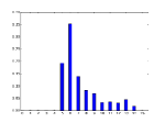
(a)

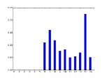
(b)

(c)

Figure 3: (a) Lung nodules, (b) Gray scale histogram (16 bins), (c) Histogram of oriented gradient. Top row is of a benign nodule, bottom is that of a malignant one.

Given an intensity lung nodule image, as in Fig. 3a, a gray scale histogram of $B$ bins is extracted by first dividing the image range in $B$ equally spaced gray scale value ranges. Then for each pixel value, the corresponding bin value is incremented by one. Finally, the obtained histogram is normalized. Here, a gray scale histogram of $16$ bins is used (i.e., $B=16$). Sample histograms of a benign and malignant nodules are shown in Fig. 3b top and bottom respectively.

III-C Oriented Gradient Histogram

The third feature type considered is image gradient histogram. The gradient information in an image provides a lot of information about the nature of the object presented in the image. Gradient magnitude and orientation based features are the most discriminant and most successfully used features in object detection and classification tasks [6]. The oriented gradient histogram is computed first by determining the image gradient (magnitude and orientation) at each pixel of the given image containing a lung nodule. Then a histogram whose bins represent gradient orientations is constructed by adding the gradient magnitude of the pixel at the corresponding histogram bin. Basically, the horizontal axis of the histogram corresponds to gradient orientation and the vertical axis corresponds to the binned gradient magnitude. Contrary to most approaches in the literature that concatenate localized histograms to keep spatial information, one global histogram per image is computed in this work to minimize its variance to image (or lung nodule) rotation. A contrast insensitive (considering only $[0^{o},180^{o}]$ magnitude orientation) oriented gradient histogram of $9$ bins is used. Sample illustrative histograms are shown in Fig. 3c.

Finally, all the three extracted feature sets, geometric, gray scale histogram, and oriented gradient histogram, are combined to create a $29$ dimensional heterogeneous feature set (denoted with $\mathbf{x}$).

IV CLASSIFIERS

Five commonly used linear and non-linear classifiers are investigated. The linear ones consist of Logistic Regression classifier and Linear Support Vector Machine. The non-linear ones include K-Nearest Neighbor, Discrete AdaBoost, and Random Forest classifiers. All the classifiers considered are supervised classifiers, which are trained using labeled positive and negative training data (for two class classification problem as in this work). Given a labeled set of $n$ training instances, $\left\{(\mathbf{x}_{i},y_{i})\right\}^{n}_{i=1}$ with $y_{i}\in\{-1,+1\}$ and $\mathbf{x}\in{\rm I\!R}{}^{d}$ (a $d$ dimensional feature vector), the classifier learns a classification rule $f:\mathbf{x}\to{}y$, that maps the feature vector $\mathbf{x}$ to its label $y$. The classifiers also have a function $h(\mathbf{x})$ that provides a continuous score that acts as a confidence indicator of positive label. In fact, the classification rule $f$ is derived from $h$ by thresholding the score with a tuned (learned) threshold value $\theta$: if the score is equal to or above $\theta$, a positive label (malignant) is assigned, and otherwise a negative label (benign) is assigned.

Each classifier’s hyper-parameters are tuned via cross-validation. This includes, the $C$ of Logistic Regression and Linear SVM, the $K$ of K-NN, decision tree depth $D$ of AdaBoost, and the number $N$ and depth $D$ of decision trees used in the Random Forest classifier (these parameters are defined according to [15]).

V EXPERIMENTS AND RESULTS

V-A Evaluation Metrics

This work deals with a binary classification task. To quantitatively evaluate a trained classifier operating on a fixed point (once best case classifier thresholds $\theta$ rules have been identified via cross validation), the following standard measures are used [17]:

$$Sensitivity:{S}_{e}=\frac{TP}{TP+FN}$$ (1)

$$Specificity:{S}_{p}=\frac{TN}{TN+FP}$$ (2)

$$Accuracy:{A}=\frac{TN+TP}{TP+TN+FN+FP}$$ (3)

$$F-measure=2*\left(\frac{{S}_{e}{S}_{p}}{{S}_{e}+{S}_{p}}\right)$$ (4)

True Positive ($TP$), False Negative ($FN$), True Negative ($TN$), and False Positive ($FP$) are defined in the obvious sense. Sensitivity characterizes how well the classifier correctly recognizes malignant nodules, and specificity that of benign nodules. Accuracy measures the proportion of total data correctly classified. The F-measure, contrary to the common formulation based on Precision-Recall, is defined here as the harmonic mean of sensitivity and specificity to provide a single measure that combines both. Sensitivity-specificity ROC curve is used to characterize classifier performance over several operating points. It is then summarized by obtaining the Area Under the Curve (AUC).

V-B Dataset

The proposed benign-malignant classification framework is primarily trained and tested using the publicly available LIDC-IDRI lung CT image dataset [5]. This dataset is of particular interest in this work because it provides diagnosis data for a subset of the subjects – we use the data from $95$ subjects for which accurate diagnostic label could be established. The nodule level diagnosis is marked as: 0 - unknown, 1 - benign, 2 - malignant (primary lung cancer), and 3 - malignant (metastatic). Furthermore, nodules with only benign and malignant labels (1,2,3) are considered which further reduced the data (all nodules with a label 0, for unknown, are not considered). This resulted in $52$ subjects with malignant nodules and $21$ subjects with benign nodules with a total of $458$ and $107$ individual lung CT slice nodules respectively (see Table II). Out of this $65\%$ are used for training and the rest are used for testing.

	unknown (0)	benign (1)	malignant (2 and 3)
# of subjects	22	21	52
# of CT slices	74	107	458
# of CT slices (train / test)	–	66 / 41	301 / 157

TABLE II: LIDC-IDRI dataset summary of nodule diagnosis information.

V-C Implementation Details

The lung nodule benign-malignant classification framework presented in this work has been completely implemented in python. The dicom data obtained from the LIDC-IDRI dataset is normalized to $[0,256)$ discrete values. When extracting histogram features (gray scale and oriented gradient), a rectangular region encompassing the union of all radiologist nodule boundary annotation with an additional $5\%$ margin to include background information is used. All described features are mean and variance normalized to approximately follow a normally distributed data. This is a common requirement for the classification algorithms used which are based on scikit-learn [15]. Given the small number of training/test data available, a 5-fold cross validation setup is used to determine model variables. Once the suitable variable is identified, the classifier is retrained using the entire training data. Finally, this trained classifier is evaluated on the test set to provide definitive evaluation metrics, both operating point metrics and ROC curve.

V-D Results

The final test results obtained using the combined heterogeneous feature set with the different classifiers, test ROC curves, are shown in Fig. 4. The AUC and operating point evaluation results are also detailed in Table III. Overall, the best AUC result is obtained by AdaBoost and is $0.94$ which is very close to a perfect score. This AdaBoost classifier also achieves the best specificity, accuracy, and F-measure. The second best results are obtained using the random forest classifier. The results obtained by the non-linear classifiers are much better than the linear classifier cases.

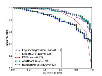
Figure 4: Test set ROC curves obtained using the combined heterogeneous features.

Classifier	Parameter(s)	AUC	Sensitivity	Specificity	Accuracy	F-measure
Logistic Regression	$C=2.0$	0.81	0.71	0.80	0.73	0.75
Linear SVM	$C=0.25$	0.82	0.72	0.80	0.74	0.76
K-NN	$K=5$	0.87	0.81	0.78	0.80	0.79
AdaBoost	$D=5$	0.94	0.82	0.93	0.84	0.87
Random Forest	$D=25$,$N=40$	0.92	0.80	0.90	0.82	0.85
Kumar et al. [10]	–	–	0.83	0.21	0.75	0.34
Kumar et al. [9]	–	–	0.79	0.76	0.78	0.77

TABLE III: Test set results obtained using the combined heterogeneous feature set with optimized classifiers and comparisons with the state-of-the-art. Best results  on each metric are highlighted.

These results are very promising. Unfortunately, due to the nature of the data used, a direct comparison with results in the literature is not valid. As described, the LIDC-IDRI diagnosis data does not provide an absolute position of the referenced nodule. This means that it is only possible to use nodule data in certainty if and only if a patient has only one identified lung nodule (which reduced the total number of subjects to use from 157 to 95). For the sake of comparison, the last two rows of Table III report state-of-the-art results in the literature obtained using the LIDC-IDRI dataset. Except the sensitivity of $83\%$, our best approach based on AdaBoost and the proposed heterogeneous features outperforms their reported results. We obtain a $9\%$ and $6\%$ improved accuracy compared to [10] and [9] respectively. We also obtain a significantly improved F-measure.

VI CONCLUSIONS AND FUTURE WORKS

This work investigated an automated framework for lung nodule benign-malignant classification based on lung CT images with annotated nodules. The experimental results presented in this work make it possible to make the following three conclusive observations based on the dataset utilized: (i) Image features provide useful cues that are useful for benign-malignant lung nodule classification, (ii) Heterogeneous features lead to improved classification accuracy, compared to the constituent counterparts, as they combine various complementary cues, and (iii) In general non-linear classifiers, especially ensemble classifiers, are better suited for lung nodule benign-malignant classification. The experimental results on the LIDC-IDRI public dataset are very encouraging correctly classifying $82\%$ of malignant and $93\%$ of benign nodules on unseen test data at best.

Possible future lines of investigations include: addition of texture image features, e.g., Local Binary Patterns (LBP), consideration of volume CT image features, and probabilistic data fusion strategies to incorporate clinical features at a higher reasoning level.

References

- [1] D.R. Aberle, A.M. Adams, C.D. Berg, W.C. Black, J.D. Clapp, and et al. Reducing lung-cancer mortality with low-dose computed tomographic screening. New England Journal of Medicine, 365:pp 395–409, 2011.
- [2] M. Aoyama, Q. Li, S. Katsuragawa, H. MacMahon, and K. Doi. Automated computerized scheme for distinction between benign and malignant solitary pulmonary nodules on chest images. Medical Physics, 29:701–708, 2002.
- [3] Samuel G. Armato, Michael B. Altman, Joel Wilkie, Shusuke Sone, Feng Li, Kunio Doi, and Arunabha S. Roy. Automated lung nodule classification following automated nodule detection on ct: A serial approach. Medical Physics, 30(6):1188–1197, 2003.
- [4] Samuel G. Armato, Lubomir Hadjiiski, and Georgia D. Tourassi et al. Guest editorial: Lungx challenge for computerized lung nodule classification: reflections and lessons learned. Journal of Medical Imaging, 2(2):020103, 2015.
- [5] Samuel G. Armato, Geoffrey McLennan, and Luc Bidaut et al. The Lung Image Database Consortium (LIDC) and Image Database Resource Initiative (IDRI): A Completed Reference Database of Lung Nodules on CT Scans. Medical Physics, 38(2):915–931, 2011.
- [6] Piotr Dollár, Ron Appel, Serge Belongie, and Pietro Perona. Fast feature pyramids for object detection. IEEE Trans. Pattern Anal. Mach. Intell., 36(8):1532–1545, 2014.
- [7] Ayman El-Baz, Garth M. Beache, Georgy Gimel’farb, Kenji Suzuki, Kazunori Okada, Ahmed Elnakib, Ahmed Soliman, and Behnous Abdollahi. Computer-aided diagnosis systems for lung cancer: Challenges and methodologies. International Journal of Biomedical Imaging, page 46 pages, 2013.
- [8] J. Ferlay, Soerjomataram I., M. Ervik, and et al. Globovan 2012 v1.0, cancer incidence and mortality worldwide. Technical report, Lyon, France, 2013.
- [9] Devinder Kumar, Mohammad Javad Shafiee, Audrey G. Chung, Farzad Khalvati, Masoom A. Haider, and Alexander Wong. Discovery radiomics for computed tomography cancer detection. CoRR, abs/1509.00117, 2015.
- [10] Devinder Kumar, Alexander Wong, and David A Clausi. Lung nodule classification using deep features in ct images. In Computer and Robot Vision (CRV), 2015 12th Conference on, pages 133–138. IEEE, 2015.
- [11] Michael C. Lee, Lilla Boroczky, Kivilcim Sungur-Stasik, Aaron D. Cann, Alain C. Borczuk, Steven M. Kawut, and Charles A. Powell. Computer-aided diagnosis of pulmonary nodules using a two-step approach for feature selection and classifier ensemble construction. Artificial Intelligence in Medicine, 50(1):43 – 53, 2010. Knowledge Discovery and Computer-Based Decision Support in Biomedicine.
- [12] Qiang Li, Feng Li, Kenji Suzuki, Junji Shiraishi, Hiroyuki Abe, Roger Engelmann, Yongkang Nie, Heber MacMahon, and Kunio Doi. Computer-aided diagnosis in thoracic {CT}. Seminars in Ultrasound, {CT} and {MRI}, 26(5):357 – 363, 2005. Update of Chest Imaging-Part I.
- [13] Hiram Madero Orozco, Osslan Osiris Vergara Villegas, Vianey Guadalupe Cruz Sánchez, Humberto de Jesús Ochoa Domínguez, and Manuel de Jesús Nandayapa Alfaro. Automated system for lung nodules classification based on wavelet feature descriptor and support vector machine. BioMedical Engineering OnLine, 14(1):1–20, 2015.
- [14] E.D. Midthun. Early diagnosis of lung cancer. F1000 Prime Reports, pages pp 5–12, 2013.
- [15] F. Pedregosa, G. Varoquaux, A. Gramfort, V. Michel, B. Thirion, O. Grisel, M. Blondel, P. Prettenhofer, R. Weiss, V. Dubourg, J. Vanderplas, A. Passos, D. Cournapeau, M. Brucher, M. Perrot, and E. Duchesnay. Scikit-learn: Machine learning in Python. Journal of Machine Learning Research, 12:2825–2830, 2011.
- [16] G.D.. Rubin, J.K. Lyo, D.S. Paik, A.J. Sherbondy, and et al. Pulmonary nodules on multi–detector row ct scans: Performance comparison of radiologists and computer-aided detection. Radiology, 234:pp 274–283, 2005.
- [17] Bowen Song, Guopeng Zhang, Wei Zhu, and Zhengrong Liang. Roc operating point selection for classification of imbalanced data with application to computer-aided polyp detection in ct colonography. International Journal of Computer Assisted Radiology and Surgery, 9(1):79–89, 2014.
- [18] A. Tartar, A. Akan, and N. Kilic. A novel approach to malignant-benign classification of pulmonary nodules by using ensemble learning classifiers. In Engineering in Medicine and Biology Society (EMBC), 2014 36th Annual International Conference of the IEEE, pages 4651–4654, Aug 2014.
- [19] Momen M. Wahidi, Joseph A. Govert, Ranjit K. Goudar, Michael K. Gould, and Douglas C. McCrory. Evidence for the treatment of patients with pulmonary nodules: When is it lung cancer?*: accp evidence-based clinical practice guidelines (2nd edition). Chest, 132(3):94S–107S, 2007.
- [20] Ted W. Way, Lubomir M. Hadjiiski, Berkman Sahiner, Heang-Ping Chan, Philip N. Cascade, Ella A. Kazerooni, Naama Bogot, and Chuan Zhou. Computer-aided diagnosis of pulmonary nodules on ct scans: Segmentation and classification using 3d active contours. Medical Physics, 33(7):2323–2337, 2006.
- [21] Ted W. Way, Berkman Sahiner, Heang-Ping Chan, Lubomir Hadjiiski, Philip N. Cascade, Aamer Chughtai, Naama Bogot, and Ella Kazerooni. Computer-aided diagnosis of pulmonary nodules on ct scans: Improvement of classification performance with nodule surface features. Medical Physics, 36(7):3086–3098, 2009.