=0.5pt \hdashlinegap=0.8pt
Low-rank tensor completion:
a Riemannian manifold preconditioning approach
Abstract
We propose a novel Riemannian manifold preconditioning approach for the tensor completion problem with rank constraint. A novel Riemannian metric or inner product is proposed that exploits the least-squares structure of the cost function and takes into account the structured symmetry that exists in Tucker decomposition. The specific metric allows to use the versatile framework of Riemannian optimization on quotient manifolds to develop preconditioned nonlinear conjugate gradient and stochastic gradient descent algorithms for batch and online setups, respectively. Concrete matrix representations of various optimization-related ingredients are listed. Numerical comparisons suggest that our proposed algorithms robustly outperform state-of-the-art algorithms across different synthetic and real-world datasets111This paper extends the earlier work Kasai & Mishra (2015) to include a stochastic gradient descent algorithm for low-rank tensor completion..
1 Introduction
This paper addresses the problem of low-rank tensor completion when the rank is a priori known or estimated. We focus on 3-order tensors in the paper, but the developments can be generalized to higher order tensors in a straightforward way. Given a tensor , whose entries are only known for some indices , where is a subset of the complete set of indices , the fixed-rank tensor completion problem is formulated as
| (1) |
where the operator if and otherwise and (with a slight abuse of notation) is the Frobenius norm. is the number of known entries. , called the multilinear rank of , is the set of the ranks of for each of mode- unfolding matrices. enforces a low-rank structure. The mode is a matrix obtained by concatenating the mode- fibers along columns, and mode- unfolding of a -order tensor is for .
Problem (1) has many variants, and one of those is extending the nuclear norm regularization approach from the matrix case Candès & Recht (2009) to the tensor case. This results in a summation of nuclear norm regularization terms, each one corresponds to each of the unfolding matrices of . While this generalization leads to good results Liu et al. (2013); Tomioka et al. (2011); Signoretto et al. (2014), its applicability to large-scale instances is not trivial, especially due to the necessity of high-dimensional singular value decomposition computations. A different approach exploits Tucker decomposition (Kolda & Bader, 2009, Section 4) of a low-rank tensor to develop large-scale algorithms for (1), e.g., in Filipović & Jukić (2013); Kressner et al. (2014).
The present paper exploits both the symmetry present in Tucker decomposition and the least-squares structure of the cost function of (1) to develop competitive algorithms. The multilinear rank constraint forms a smooth manifold (Kressner et al., 2014). To this end, we use the concept of manifold preconditioning. While preconditioning in unconstrained optimization is well studied (Nocedal & Wright, 2006, Chapter 5), preconditioning on constraints with symmetries, owing to non-uniqueness of Tucker decomposition Kolda & Bader (2009), is not straightforward. We build upon the recent work Mishra & Sepulchre (2016) that suggests to use preconditioning with a tailored metric (inner product) in the Riemannian optimization framework on quotient manifolds Absil et al. (2008); Edelman et al. (1998); Mishra & Sepulchre (2016). The differences with respect to the work of Kressner et al. (2014), which also exploits the manifold structure, are twofold. (i) Kressner et al. (2014) exploit the search space as an embedded submanifold of the Euclidean space, whereas we view it as a product of simpler search spaces with symmetries. Consequently, certain computations have straightforward interpretation. (ii) Kressner et al. (2014) work with the standard Euclidean metric, whereas we use a metric that is tuned to the least-squares cost function, thereby inducing a preconditioning effect. This novel idea of using a tuned metric leads to a superior performance of our algorithms. They also connect to state-of-the-art algorithms proposed in Ngo & Saad (2012); Wen et al. (2012); Mishra & Sepulchre (2014); Boumal & Absil (2015).
The paper is organized as follows. Section 2 discusses the two fundamental structures of symmetry and least-squares associated with (1) and proposes a novel metric that captures the relevant second order information of the problem. The optimization-related ingredients on the Tucker manifold are developed in Section 3. The cost function specific ingredients are developed in Section 4. The final formulas are listed in Table 1, which allow to develop preconditioned conjugate gradient descent algorithm in the batch setup and stochastic gradient descent algorithm in the online setup. In Section 5, numerical comparisons with state-of-the-art algorithms on various synthetic and real-world benchmarks suggest a superior performance of our proposed algorithms. Our proposed algorithms are implemented in the Matlab toolbox Manopt Boumal et al. (2014). The concrete proofs of propositions, development of optimization-related ingredients, and additional numerical experiments are shown in Sections A and B, respectively, of the supplementary material file. The Matlab codes for first and second order implementations, e.g., gradient descent and trust-region methods, are available at https://bamdevmishra.com/codes/tensorcompletion/.
2 Exploiting the problem structure
Construction of efficient algorithms depends on properly exploiting the problem structure. To this end, we focus on two fundamental structures in (1): symmetry in the constraints and the least-squares structure of the cost function. Finally, a novel metric is proposed.
The symmetry structure in Tucker decomposition. The Tucker decomposition of a tensor of rank r (=) is
| (2) |
where for belongs to the Stiefel manifold of matrices of size with orthogonal columns and Kolda & Bader (2009). Here, computes the d-mode product of a tensor and a matrix . Tucker decomposition (2) is not unique as remains unchanged under the transformation
| (3) |
for all , which is the set of orthogonal matrices of size of . The classical remedy to remove this indeterminacy is to have additional structures on like sparsity or restricted orthogonal rotations (Kolda & Bader, 2009, Section 4.3). In contrast, we encode the transformation (3) in an abstract search space of equivalence classes, defined as,
| (4) |
The set of equivalence classes is the quotient manifold Lee (2003)
| (5) |
where is called the total space (computational space) that is the product space
| (6) |
Due to the invariance (3), the local minima of (1) in are not isolated, but they become isolated on . Consequently, the problem (1) is an optimization problem on a quotient manifold for which systematic procedures are proposed in Absil et al. (2008); Edelman et al. (1998). A requirement is to endow endow with a Riemannian structure, which conceptually translates (1) into an unconstrained optimization problem over the search space . We call , defined in (5), the Tucker manifold as it results from Tucker decomposition.
The least-squares structure of the cost function. In unconstrained optimization, the Newton method is interpreted as a scaled steepest descent method, where the search space is endowed with a metric (inner product) induced by the Hessian of the cost function Nocedal & Wright (2006). This induced metric (or its approximation) resolves convergence issues of first order optimization algorithms. Analogously, finding a good inner product for (1) is of profound consequence. Specifically for the case of quadratic optimization with rank constraint (matrix case), Mishra and Sepulchre Mishra & Sepulchre (2016) propose a family of Riemannian metrics from the Hessian of the cost function. Applying this approach directly for the particular cost function of (1) is computationally costly. To circumvent the issue, we consider a simplified cost function by assuming that contains the full set of indices, i.e., we focus on to propose a metric candidate. Applying the metric tuning approach of Mishra & Sepulchre (2016) to the simplified cost function leads to a family of Riemannian metrics. A good trade-off between computational cost and simplicity is by considering only the block diagonal elements of the Hessian of . It should be noted that the cost function is convex and quadratic in . Consequently, it is also convex and quadratic in the arguments individually. Equivalently, the block diagonal approximation of the Hessian of in is
| (7) |
where is the mode- unfolding of and is assumed to be full rank. is the Kronecker product. The terms for are positive definite when , , and , which is a reasonable assumption.
A novel Riemannian metric. An element in the total space has the matrix representation . Consequently, the tangent space is the Cartesian product of the tangent spaces of the individual manifolds of (6), i.e., has the matrix characterization Edelman et al. (1998)
| (8) |
From the earlier discussion on symmetry and least-squares structure, we propose the novel metric or inner product
| (9) |
where are tangent vectors with matrix characterizations, shown in (8), and , respectively and is the Euclidean inner product. It should be emphasized that the proposed metric (9) is induced from (7).
3 Notions of manifold optimization
Each point on a quotient manifold represents an entire equivalence class of matrices in the total space. Abstract geometric objects on the quotient manifold call for matrix representatives in the total space . Similarly, algorithms are run in the total space , but under appropriate compatibility between the Riemannian structure of and the Riemannian structure of the quotient manifold , they define algorithms on the quotient manifold. The key is endowing with a Riemannian structure. Once this is the case, a constraint optimization problem, for example (1), is conceptually transformed into an unconstrained optimization over the Riemannian quotient manifold (5). Below we briefly show the development of various geometric objects that are required to optimize a smooth cost function on the quotient manifold (5) with first order methods, e.g., conjugate gradients.
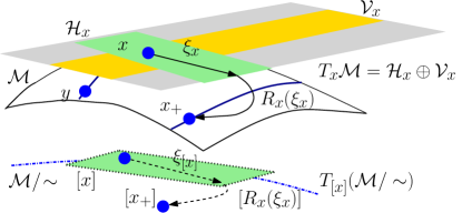
Quotient manifold representation and horizontal lifts. Figure 1 illustrates a schematic view of optimization with equivalence classes, where the points and in belong to the same equivalence class (shown in solid blue color) and they represent a single point on the quotient manifold . The abstract tangent space at has the matrix representation in , but restricted to the directions that do not induce a displacement along the equivalence class . This is realized by decomposing into two complementary subspaces, the vertical and horizontal subspaces. The vertical space is the tangent space of the equivalence class . On the other hand, the horizontal space is the orthogonal subspace to in the sense of the metric (9). Equivalently, . The horizontal subspace provides a valid matrix representation to the abstract tangent space . An abstract tangent vector at has a unique element that is called its horizontal lift.
A Riemannian metric at defines a Riemannian metric , i.e., on the quotient manifold , if does not depend on a specific representation along the equivalence class . Here, and are tangent vectors in , and and are their horizontal lifts in at , respectively. Equivalently, the definition of the Riemannian metric is well posed when for all , where and are the horizontal lifts of along the same equivalence class . This holds true for the proposed metric (9) as shown in Proposition 1. From Absil et al. (2008), endowed with the Riemannian metric (9), the quotient manifold is a Riemannian submersion of . The submersion principle allows to work out concrete matrix representations of abstract object on , e.g., the gradient of a smooth cost function Absil et al. (2008).
Starting from an arbitrary matrix (with appropriate dimensions), two linear projections are needed: the first projection is onto the tangent space , while the second projection is onto the horizontal subspace . The computation cost of these is .
The tangent space projection is obtained by extracting the component normal to in the ambient space. The normal space has the matrix characterization . Symmetric matrices for all parameterize the normal space. Finally, the operator is given as follows.
Proposition 2.
The Lyapunov equations in Proposition 2 are solved efficiently with the Matlab’s lyap routine.
The horizontal space projection of a tangent vector is obtained by removing the component along the vertical space. The vertical space has the matrix characterization . Skew symmetric matrices for all parameterize the vertical space. Finally, the horizontal projection operator is given as follows.
Proposition 3.
The coupled Lyapunov equations (11) are solved efficiently with the Matlab’s pcg routine that is combined with a specific symmetric preconditioner resulting from the Gauss-Seidel approximation of (11). For the variable , the preconditioner is of the form . Similarly, for the variables and .
Retraction. A retraction is a mapping that maps vectors in the horizontal space to points on the search space and satisfies the local rigidity condition Absil et al. (2008). It provides a natural way to move on the manifold along a search direction. Because the total space has the product nature, we can choose a retraction by combining retractions on the individual manifolds, i.e., where and extracts the orthogonal factor of a full column rank matrix, i.e., . The retraction defines a retraction on the quotient manifold , as the equivalence class does not depend on specific matrix representations of and , where is the horizontal lift of the abstract tangent vector .
Vector transport. A vector transport on a manifold is a smooth mapping that transports a tangent vector at to a vector in the tangent space at a point . It is defined by the symbol . It generalizes the classical concept of translation of vectors in the Euclidean space to manifolds (Absil et al., 2008, Section 8.1.4). The horizontal lift of the abstract vector transport on has the matrix characterization , where and are the horizontal lifts in of and that belong to . and are projectors defined in Propositions 2 and 3. The computational cost of transporting a vector solely depends on the projection and retraction operations.
| Matrix representation | |
|---|---|
| \hdashlineComputational space | |
| \hdashlineGroup action | |
| \hdashlineQuotient space | |
| \hdashlineAmbient space | |
| \hdashlineTangent vectors in | |
| : | |
| \hdashlineMetric for | |
| any | |
| \hdashlineVertical tangent vectors | |
| in | |
| \hdashlineHorizontal tangent vectors | |
| in | |
| \hdashline projects an ambient | |
| vector | , where for are computed |
| onto | by solving Lyapunov equations as in (10). |
| \hdashline projects a tangent | |
| vector onto | , is computed in (11). |
| \hdashlineFirst order derivative of | |
| where . | |
| \hdashlineRetraction | |
| \hdashlineHorizontal lift of the | |
| vector transport |
4 Riemannian algorithms for (1)
We propose two Riemannian preconditioned algorithms for the tensor completion problem (1) that are based on the developments in Section 3. The preconditioning effect follows from the specific choice of the metric (9). In the batch setting, we use the off-the-shelf conjugate gradient implementation of Manopt for any smooth cost function Boumal et al. (2014). A complete description of the Riemannian nonlinear conjugate gradient method is in (Absil et al., 2008, Chapter 8). In the online setting, we use the stochastic gradient descent implementation (Bonnabel, 2013). For fixed rank, theoretical convergence of the Riemannian algorithms are to a stationary point, and the convergence analysis follows from Sato & Iwai (2015); Ring & Wirth (2012); Bonnabel (2013). However, as simulations show, convergence to global minima is observed in many challenging instances.
In addition to the manifold-related ingredients in Section 3, the ingredients needed are the cost function specific ones. To this end, we show the computation of the Riemannian gradient as well as a way to compute an initial guess for the step-size, which is used in the conjugate gradient method. The concrete formulas are shown in Table 1.
Riemannian gradient computation. Let be the mean square error function of (1), and be an auxiliary sparse tensor variable that is interpreted as the Euclidean gradient of in . The partial derivatives of with respect to are computed in terms of the unfolding matrices . Due to the specific scaled metric (9), the partial derivatives are further scaled by , denoted as (after scaling). Finally, from the Riemannian submersion theory (Absil et al., 2008, Section 3.6.2), the horizontal lift of is equal to . The total numerical cost of computing the Riemannian gradient depends on computing the partial derivatives, which is .
Proposition 4.
Initial guess for the step-size. Following Mishra & Sepulchre (2014); Vandereycken (2013); Kressner et al. (2014), the least-squares structure of the cost function in (1) is exploited to compute a linearized step-size guess efficiently along a search direction by considering a polynomial approximation of degree over the manifold. Given a search direction , the step-size guess is , which has a closed-form expression and the numerical cost of computing it is .
Stochastic gradient descent in online setting. In the online setting, we update every time a frontal slice, i.e., a matrix , is randomly sampled from . Equivalently, we assume that the tensor grows along the third dimension. More concretely, we calculate the rank-one Riemannian gradient (12) for the input slice. are updated by taking a step along the negative Riemannian gradient direction. Subsequently, we retract using . A popular formula for the step-size at -th update is , where is the initial step-size and is a fixed reduction factor. Following Bottou (2012), we select in the pre-training phase using a small sample size of a training set. is fixed to .
Computational cost. The total computational cost per iteration of our proposed conjugate gradient implementation is , where is the number of known entries. It should be stressed that the computational cost of our conjugate gradient implementation is equal to that of (Kressner et al., 2014). In the online setting, each stochastic gradient descent update costs , where is the number of known entries of the current frontal slice of the incomplete tensor , and is the number of slices that we have seen along direction.
5 Numerical comparisons
In the batch setting, we show a number of numerical comparisons of our proposed conjugate gradient algorithm with state-of-the-art algorithms that include TOpt Filipović & Jukić (2013) and geomCG Kressner et al. (2014), for comparisons with Tucker decomposition based algorithms, and HaLRTC Liu et al. (2013), Latent Tomioka et al. (2011), and Hard Signoretto et al. (2014) as nuclear norm minimization algorithms. In the online setting, we compare our proposed stochastic gradient descent algorithm with CANDECOMP/PARAFAC based TeCPSGD Mardani et al. (2015) and OLSTEC Kasai (2016). All simulations are performed in Matlab on a 2.6 GHz Intel Core i7 machine with 16 GB RAM. For specific operations with unfoldings of , we use the mex interfaces for Matlab that are provided by the authors of geomCG. For large-scale instances, our algorithm is only compared with geomCG as others cannot handle them. Cases S and R are for batch instances, whereas Case O is for online instances.
Since the dimension of the space of a tensor of rank is , we randomly and uniformly select known entries based on a multiple of the dimension, called the over-sampling (OS) ratio, to create the train set . Algorithms are initialized randomly, as suggested in Kressner et al. (2014), and are stopped when either the mean square error (MSE) on the train set is below or the number of iterations exceeds . We also evaluate the mean square error on a test set , which is different from . Five runs are performed in each scenario and the plots show all of them. The time plots are shown with standard deviations. It should be noted that we show most numerical comparisons on the test set as it allows to compare with nuclear norm minimization algorithms, which optimize a different (training) cost function. Additional plots are provided as supplementary material.
 (a) Case S1: comparison between metrics (train error).
 (b) Case S2: r = .
 (c) Case S2: r = .
|
 (d) Case S3.
 (e) Case S4: OS = .
 (f) Case S5: CN = .
|
 (g) Case S6: noisy data.
 (h) Case S7: rectangular tensors.
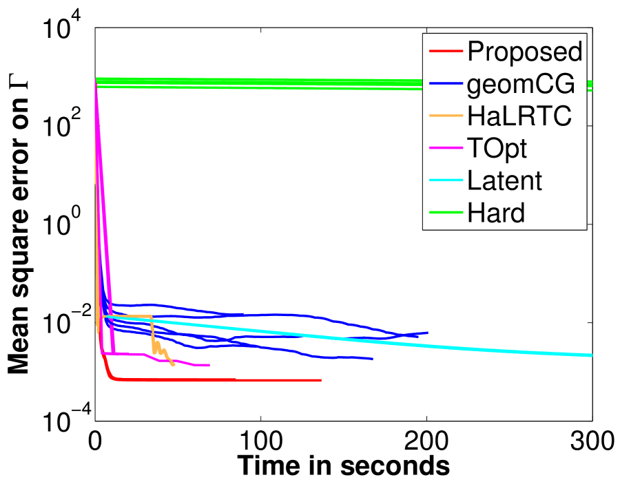
 (i) Case R1: Ribeira, OS = 11.
|
| Ribeira | OS = | OS = | ||
|---|---|---|---|---|
| \hdashline Algorithm | Time | MSE on | Time | MSE on |
| Proposed | ||||
| \hdashlinegeomCG | ||||
| \hdashlineHaLRTC | ||||
| \hdashlineTOpt | ||||
| \hdashlineLatent | ||||
| \hdashlineHard | ||||
| MovieLens-10M | Proposed | geomCG | ||
| \hdashline r | Time | MSE on | Time | MSE on |
| \hdashline | ||||
| \hdashline | ||||
| \hdashline | ||||
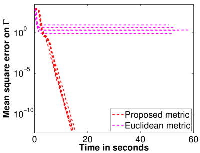
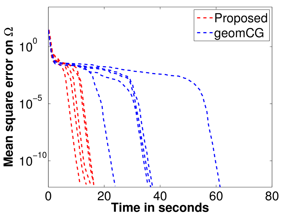
Case S1: comparison with the Euclidean metric. We first show the benefit of the proposed metric (9) over the conventional choice of the Euclidean metric that exploits the product structure of and symmetry (3). This is defined by combining the individual natural metrics for and . For simulations, we randomly generate a tensor of size and rank . OS is . For simplicity, we compare gradient descent algorithms with Armijo backtracking linesearch for both the metric choices. Figure 2(a) shows that the algorithm with the metric (9) gives a superior performance in train error than that of the conventional metric choice.
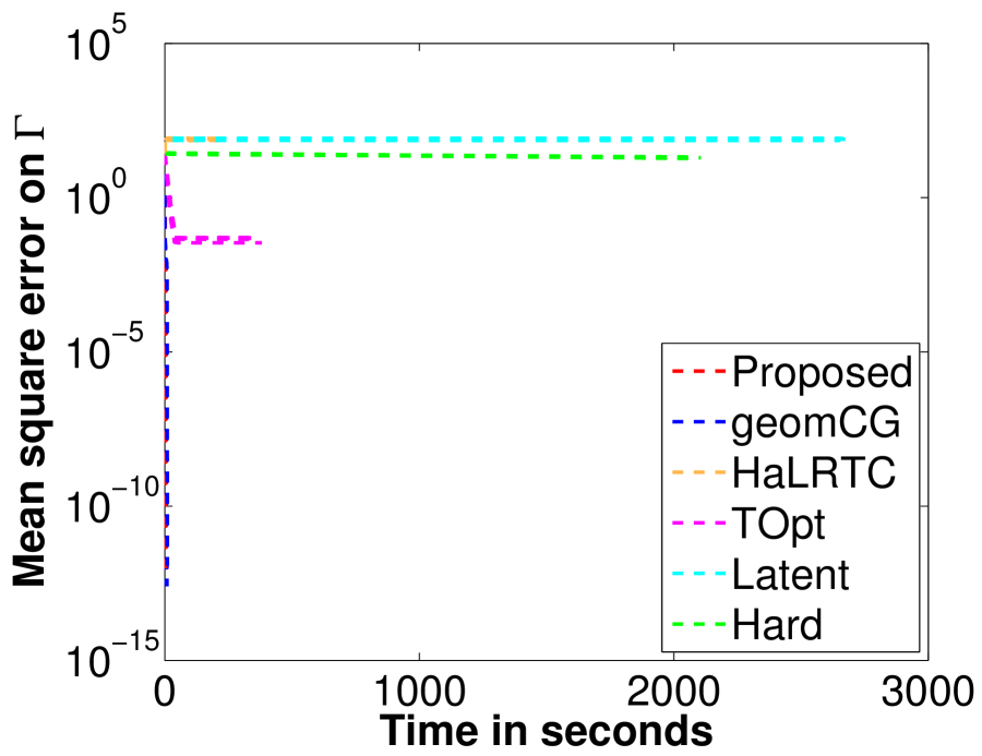
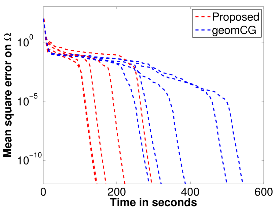
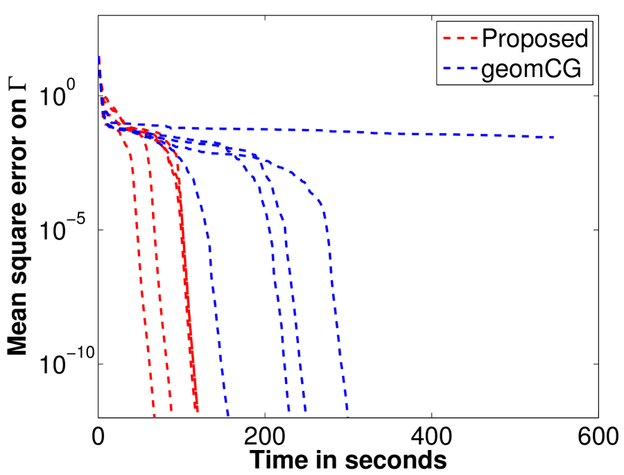
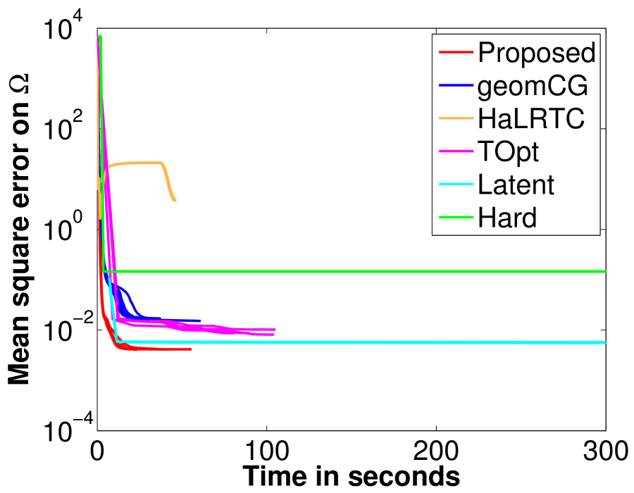
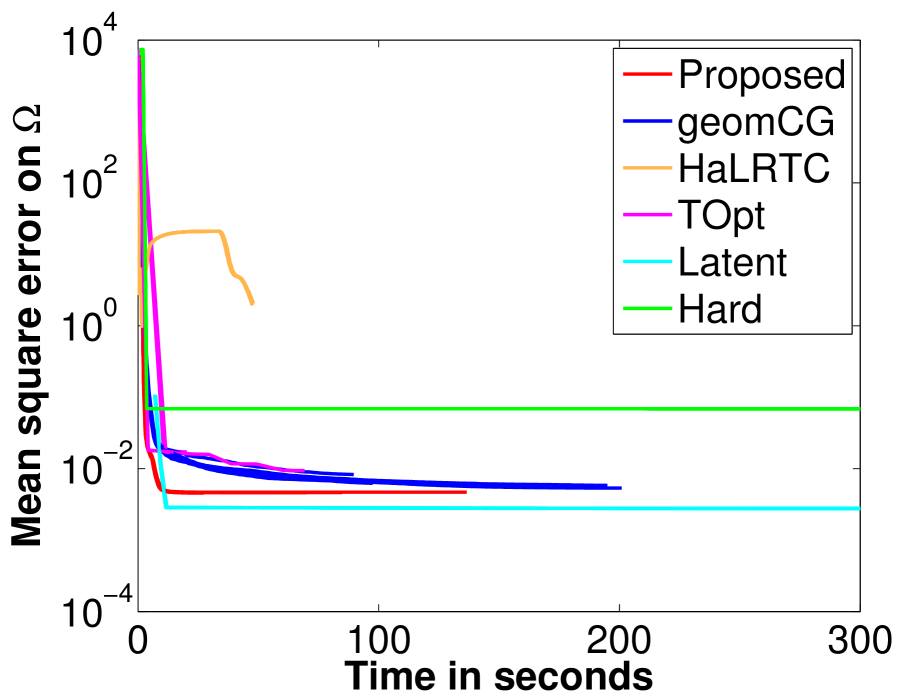
Case S2: small-scale instances. Small-scale tensors of size , , and and rank are considered. OS is . Figure 2(b) shows that our proposed algorithm has faster convergence than others. In Figure 2(c), the lowest test errors are obtained by our proposed algorithm and geomCG.
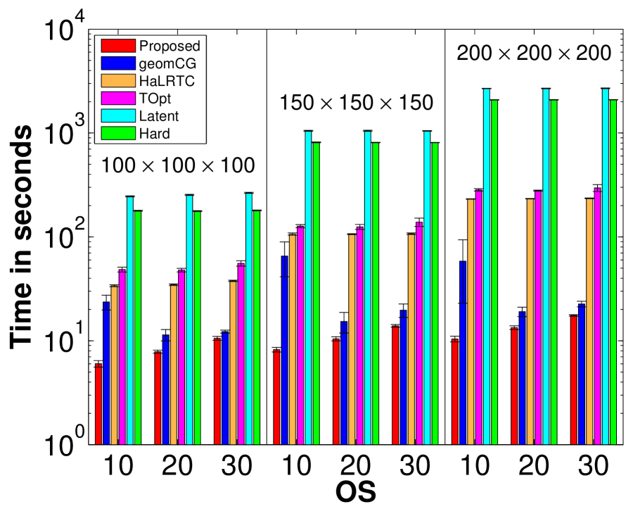
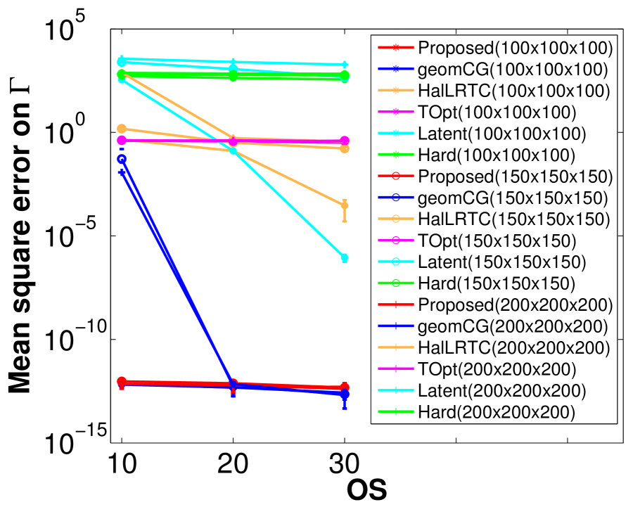
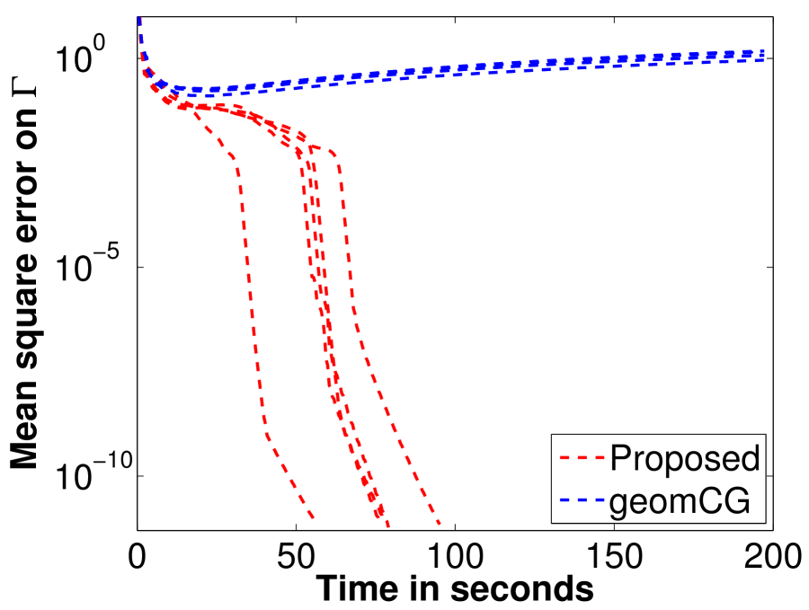
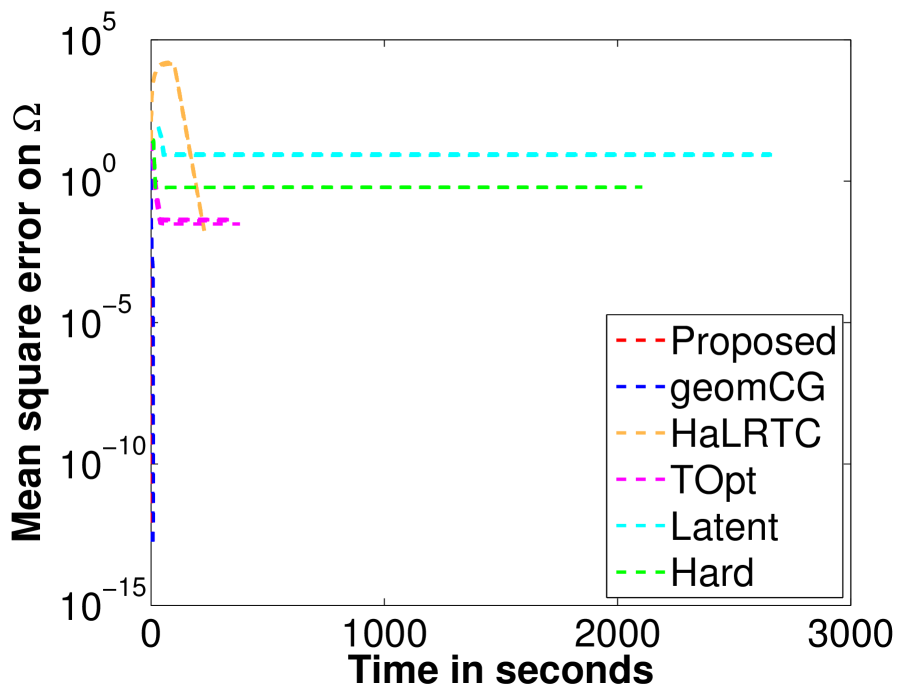
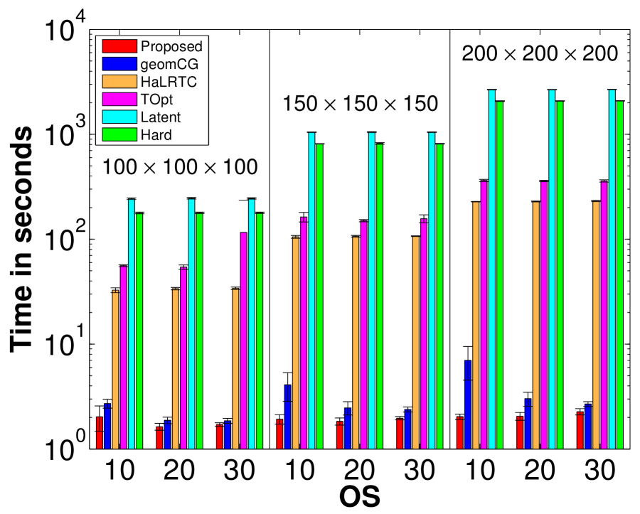
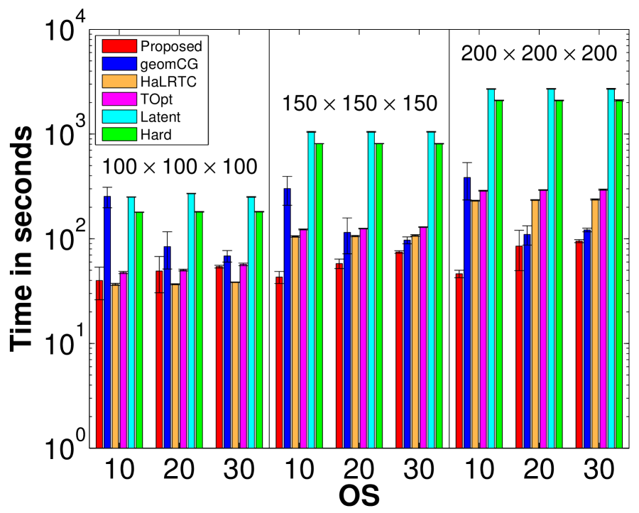
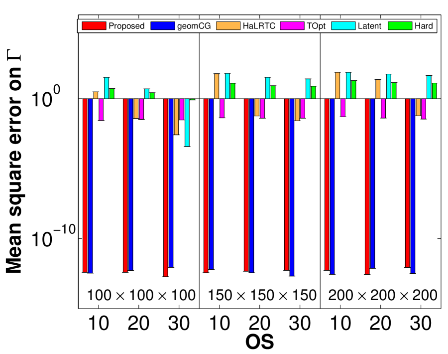
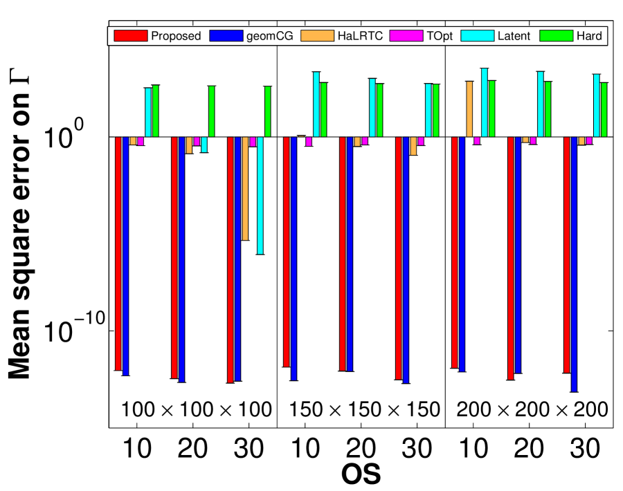
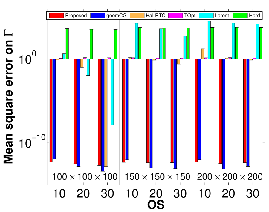
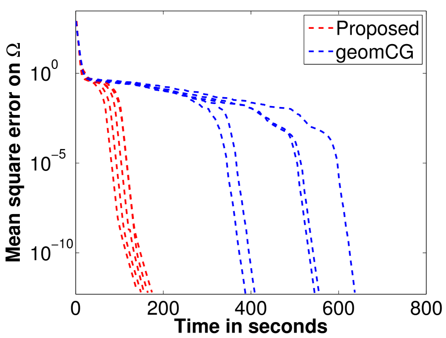
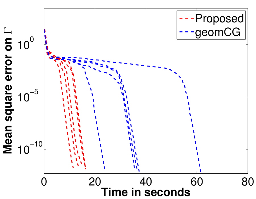
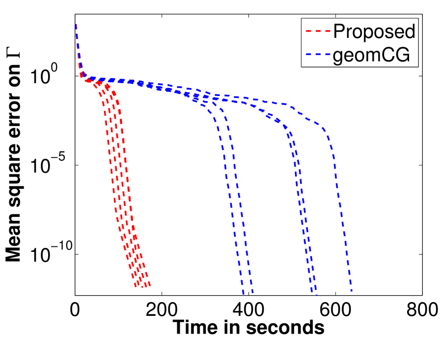
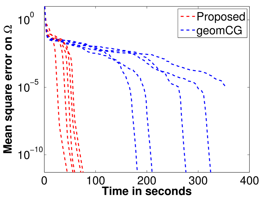
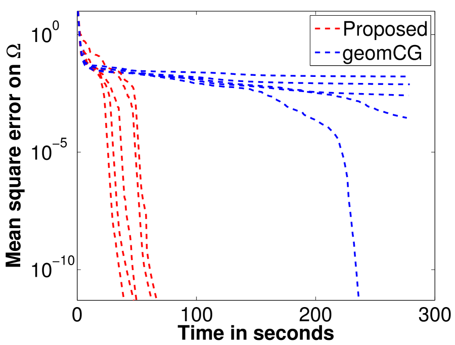
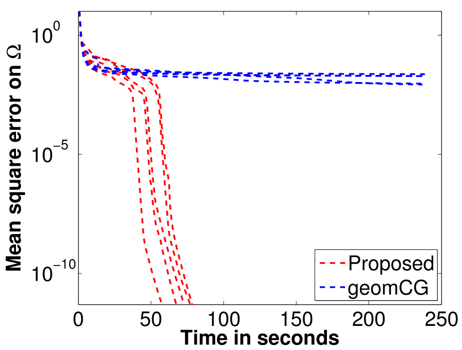
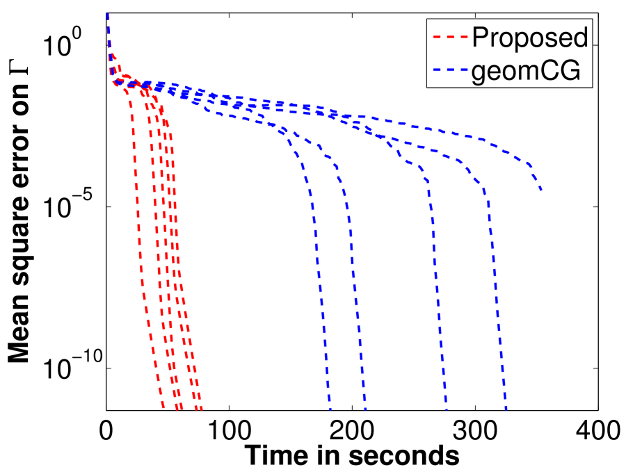
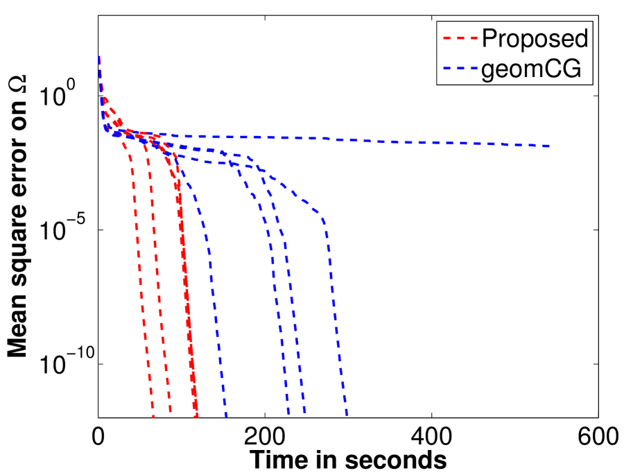
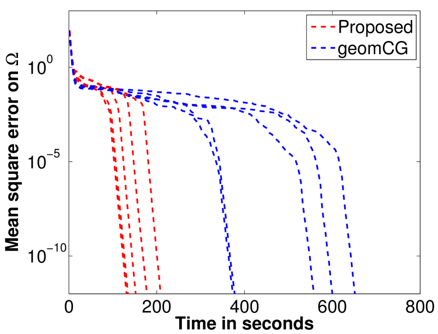
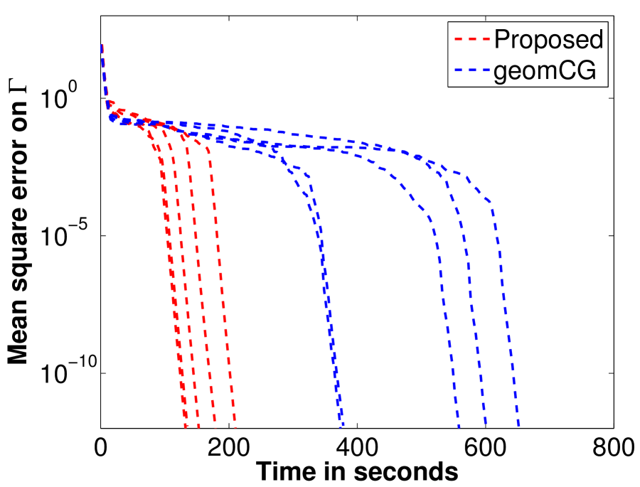
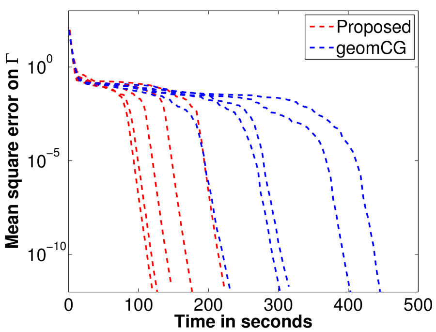
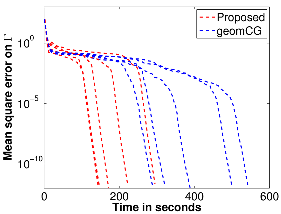
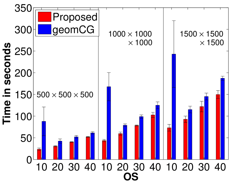
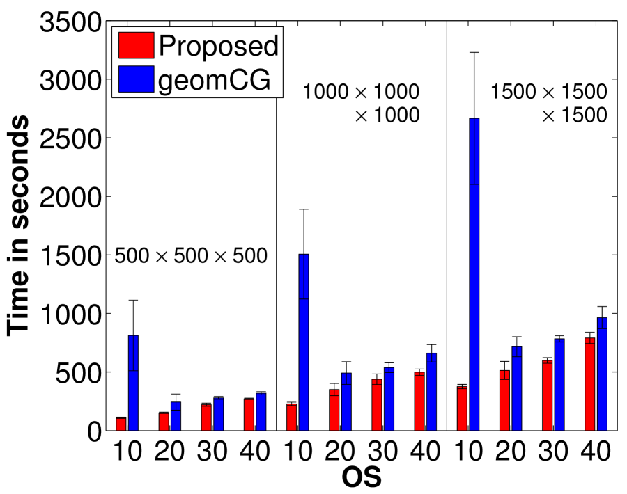
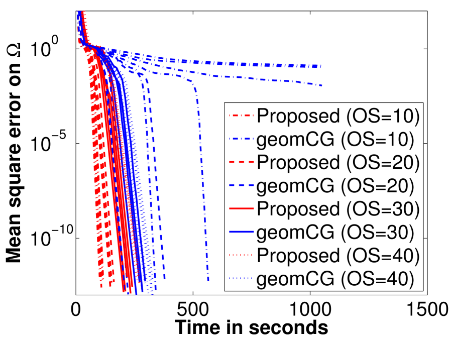
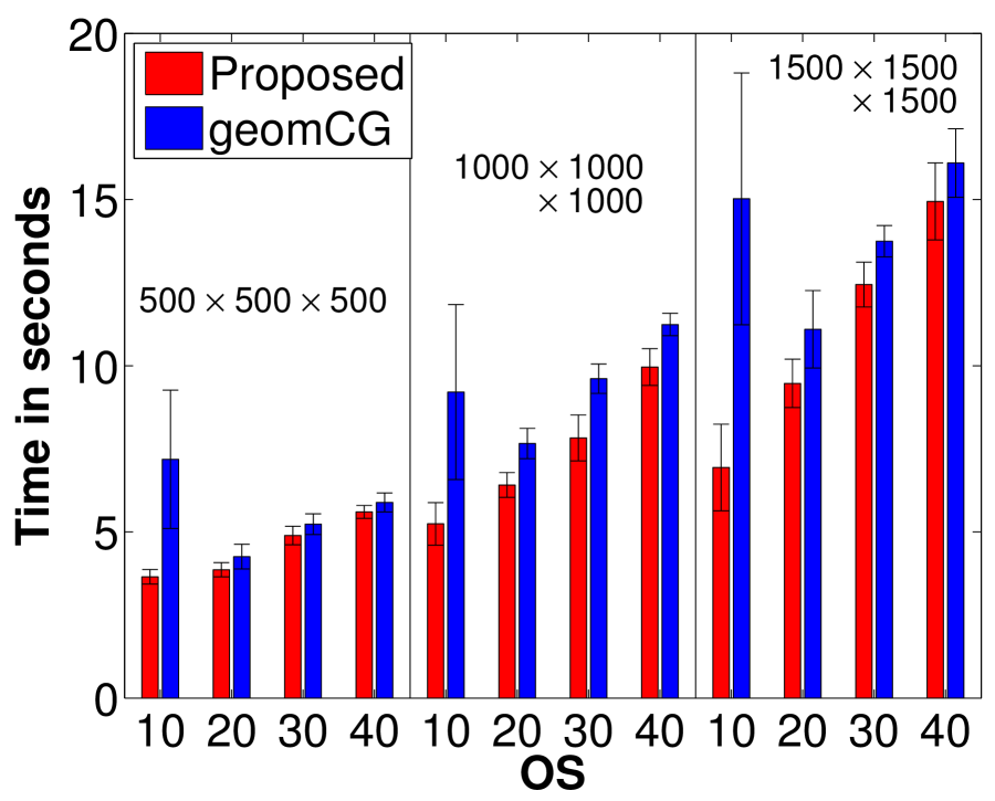
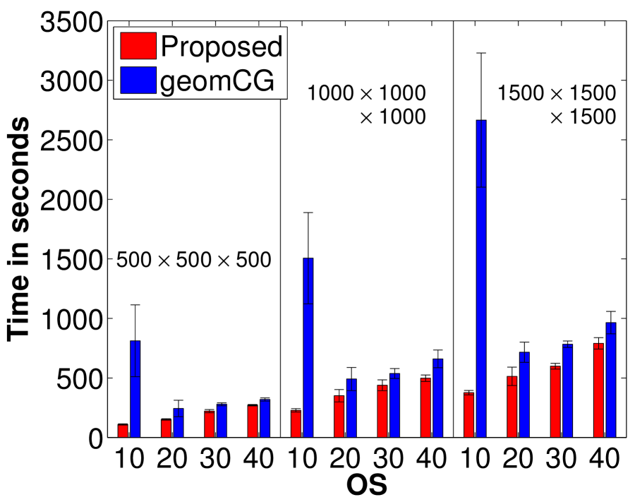
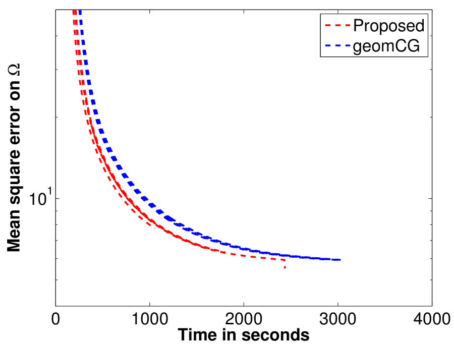
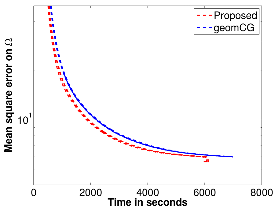
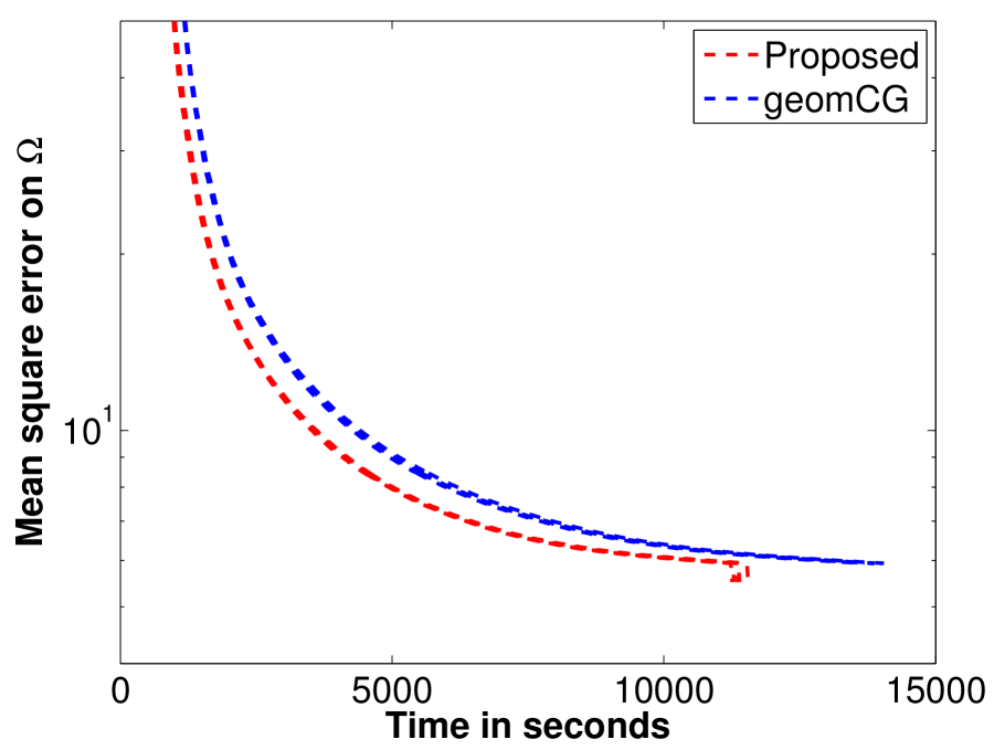
Case S3: large-scale instances. We consider large-scale tensors of size , , and and ranks and . OS is . Our proposed algorithm outperforms geomCG in Figure 2(d).
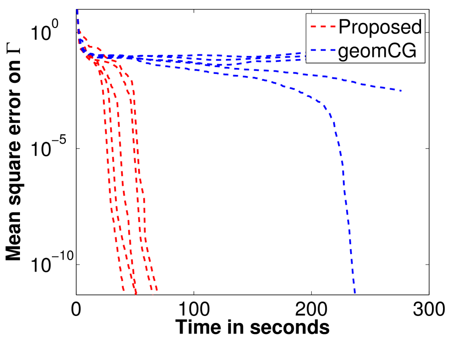
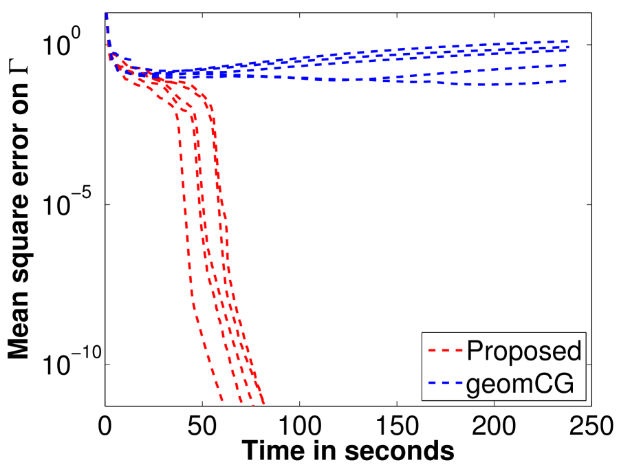
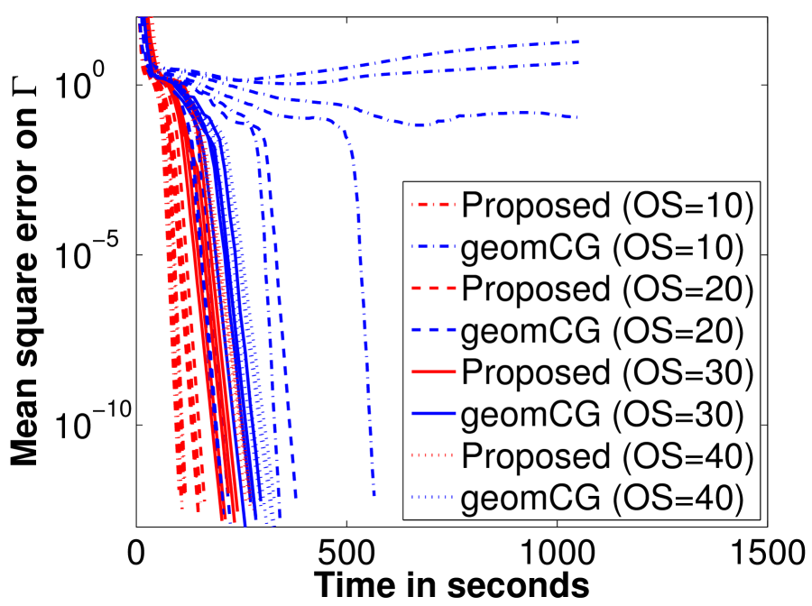
Case S4: influence of low sampling. We look into problem instances from scarcely sampled data, e.g., OS is . The test requires completing a tensor of size and rank . Figure 2(e) shows the superior performance of the proposed algorithm against geomCG. Whereas the test error increases for geomCG, it decreases for the proposed algorithm.
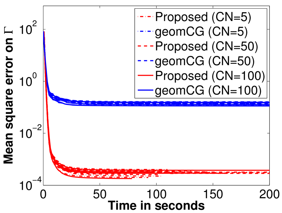
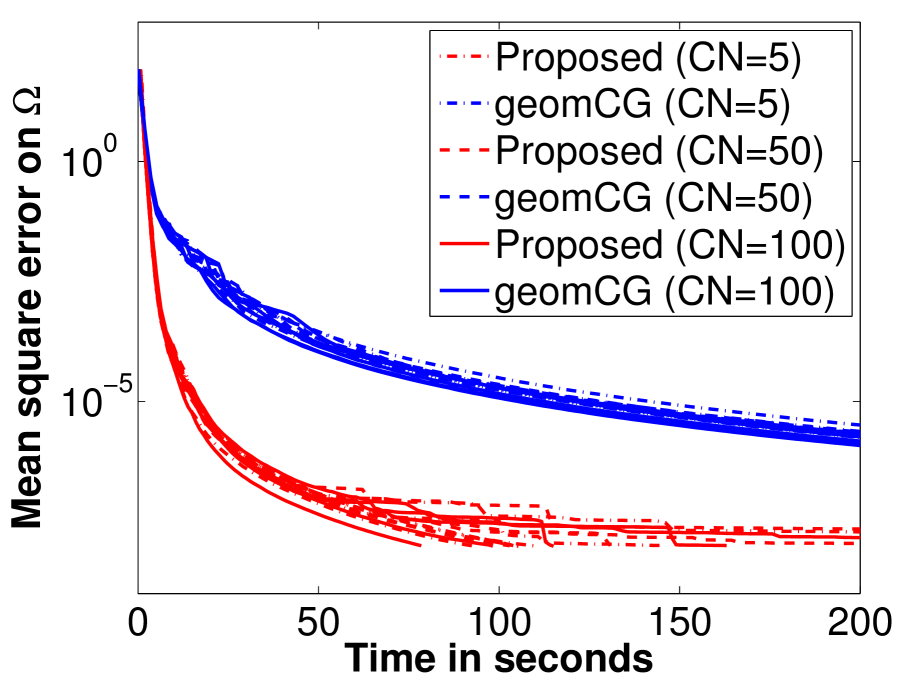
Case S5: influence of ill-conditioning and low sampling. We consider the problem instance of Case S4 with . Additionally, for generating the instance, we impose a diagonal core with exponentially decaying positive values of condition numbers (CN) , , and . Figure 2(f) shows that the proposed algorithm outperforms geomCG for all the considered CN values.
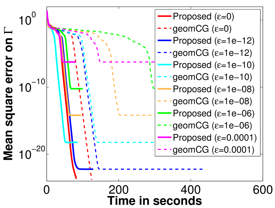
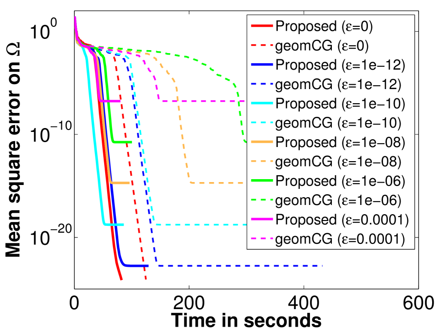
Case S6: influence of noise. We evaluate the convergence properties of algorithms under the presence of noise by adding scaled Gaussian noise to as in Kressner et al. (2014). The different noise levels are . In order to evaluate for , the stopping threshold on the MSE of the train set is lowered to . The tensor size and rank are same as in Case S4 and OS is . Figure 2(g) shows that the test error for each is almost identical to the Kressner et al. (2014), but our proposed algorithm converges faster than geomCG.
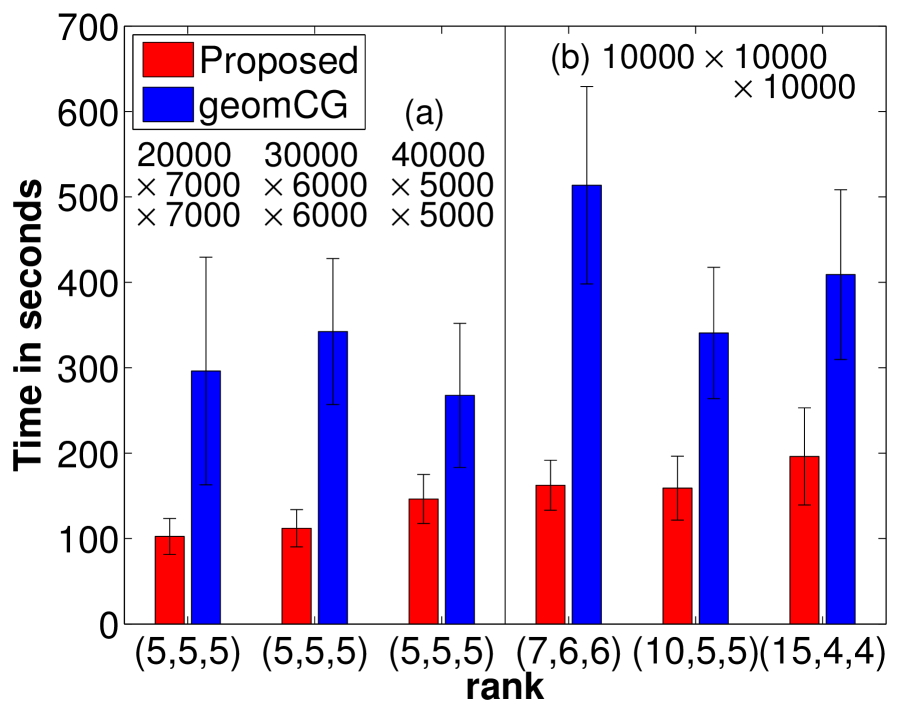
Case S7: rectangular instances. We consider instances where the dimensions and ranks along certain modes are different than others. Two cases are considered. Case (7.a) considers tensors size , , and with rank . Case (7.b) considers a tensor of size with ranks , , and . In all the cases, the proposed algorithm converges faster than geomCG as shown in Figure 2(h).
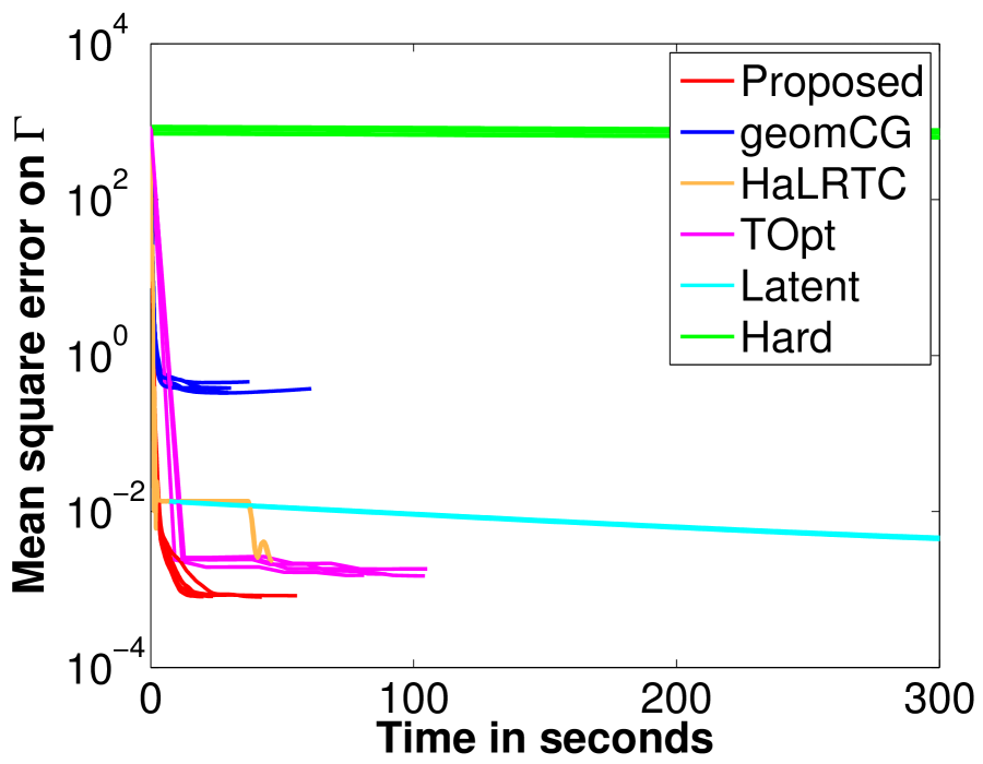
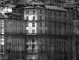
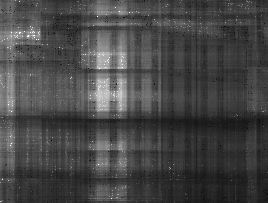
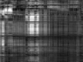
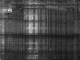
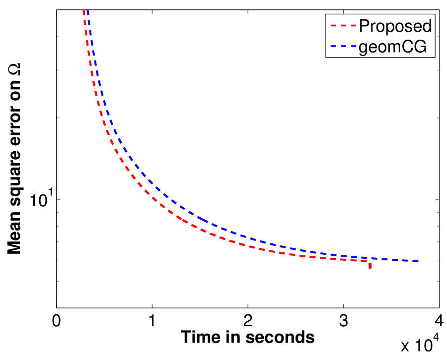
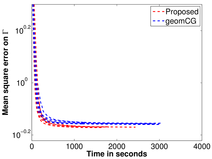
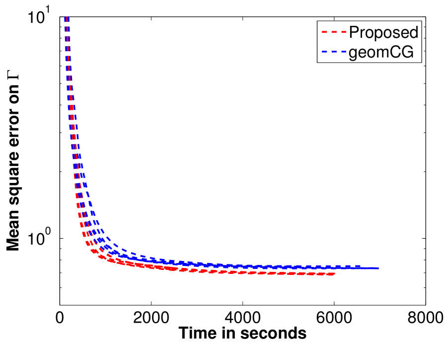
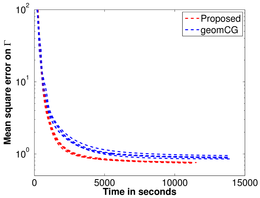
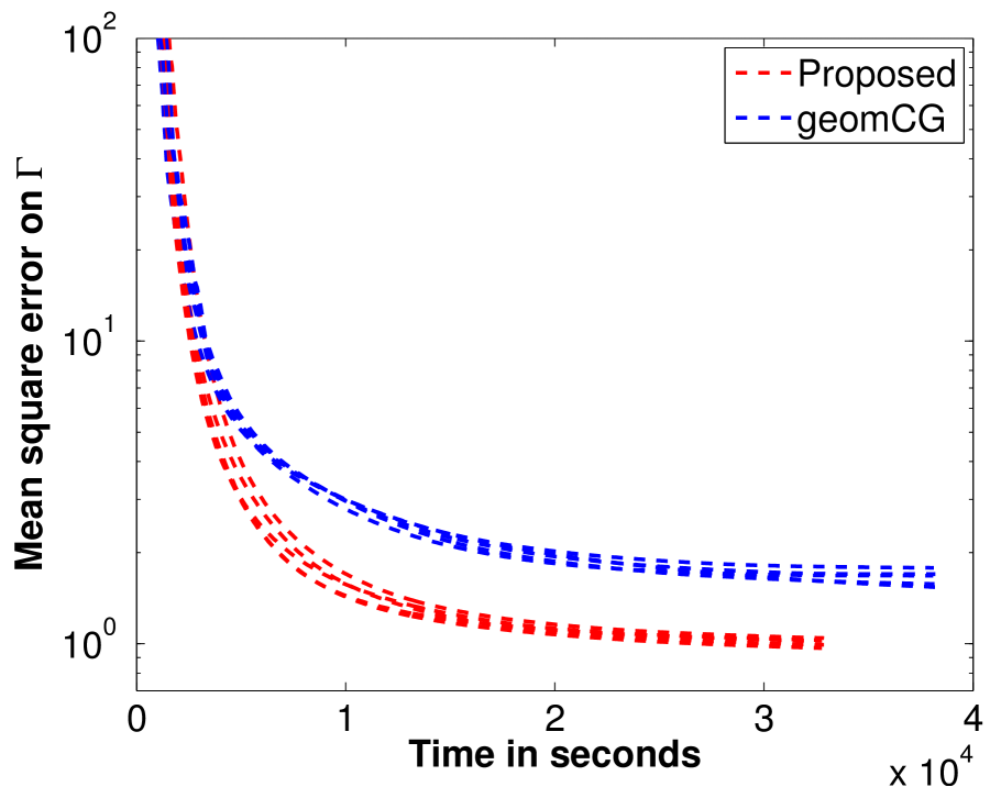
Case R1: hyperspectral image. We consider the hyperspectral image “Ribeira” Foster et al. (2007) discussed in Signoretto et al. (2011); Kressner et al. (2014). The tensor size is , where each slice corresponds to a particular image measured at a different wavelength. As suggested in Signoretto et al. (2011); Kressner et al. (2014), we resize it to . We perform five random samplings of the pixels based on the OS values and , corresponding to the rank r= adopted in Kressner et al. (2014). This set is further randomly split into //–train/validation/test partitions. The algorithms are stopped when the MSE on the validation set starts to increase. While corresponds to the observation ratio of studied in Kressner et al. (2014), considers a challenging scenario with the observation ratio of . Figures 2(i) shows the good performance of our algorithm. Table 2 compiles the results.
Case R2: MovieLens-10M222http://grouplens.org/datasets/movielens/.. This dataset contains ratings corresponding to users and movies. We split the time into -days wide bins results, and finally, get a tensor of size . The fraction of known entries is less than . The completion task on this dataset reveals periodicity of the latent genres. We perform five random //–train/validation/test partitions. The maximum iteration threshold is set to . In Table 2, our proposed algorithm consistently gives lower test errors than geomCG across different ranks.
 (a) Case O: synthetic dataset.
 (b) Case O: Airport Hall dataset.
|
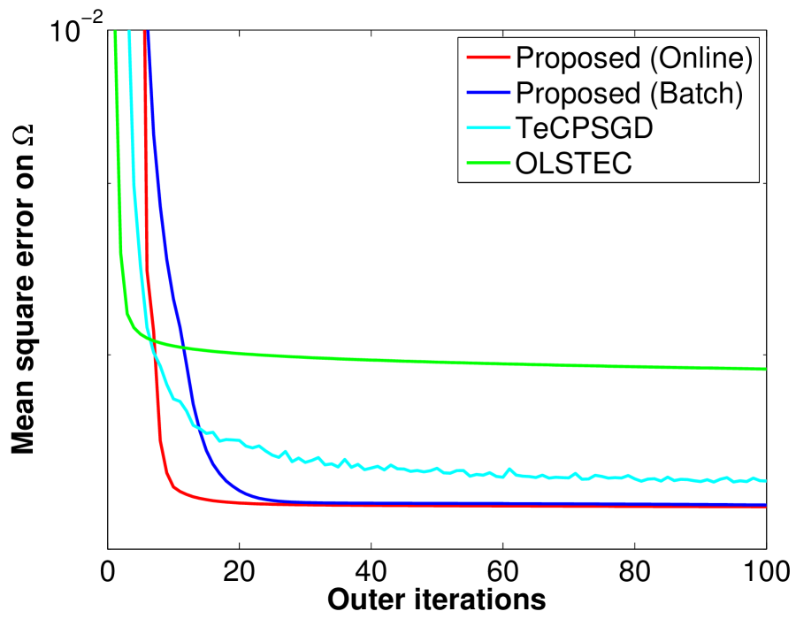
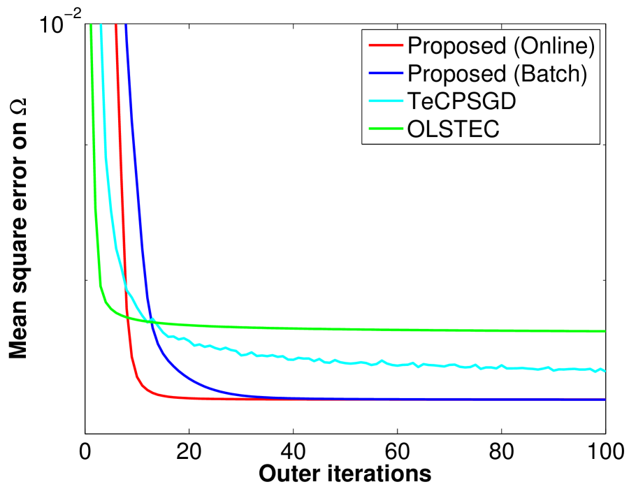
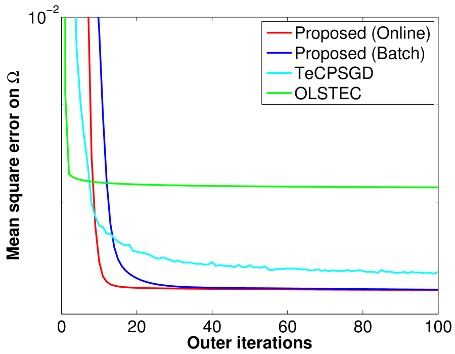
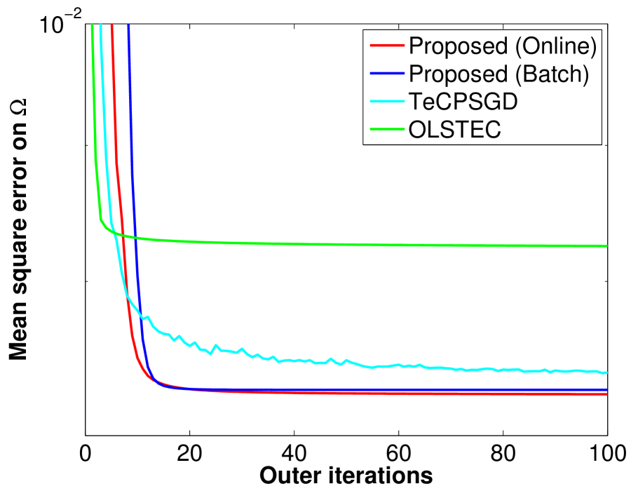
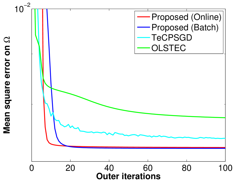
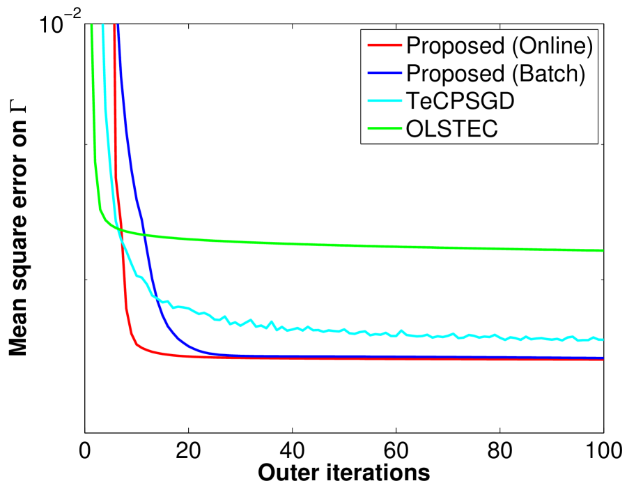
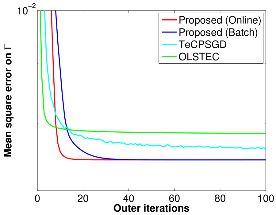
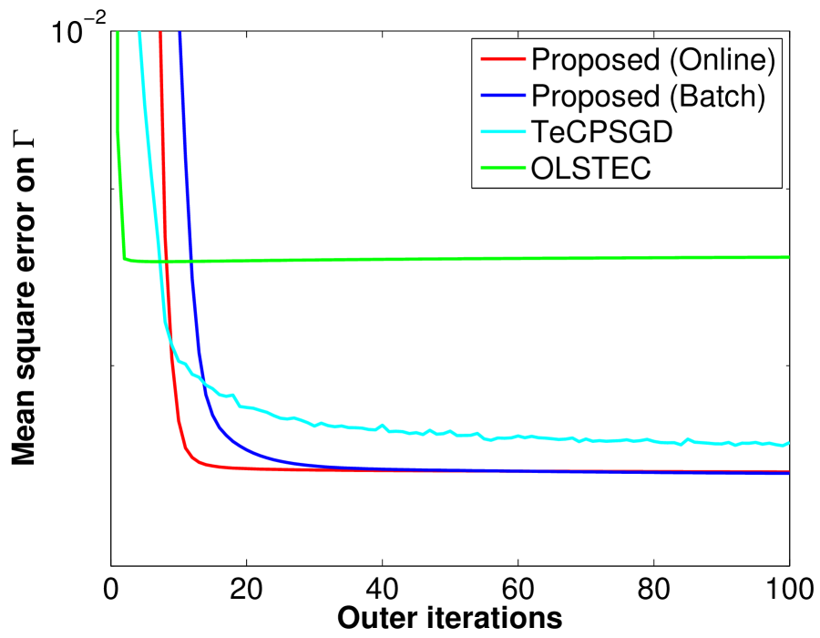
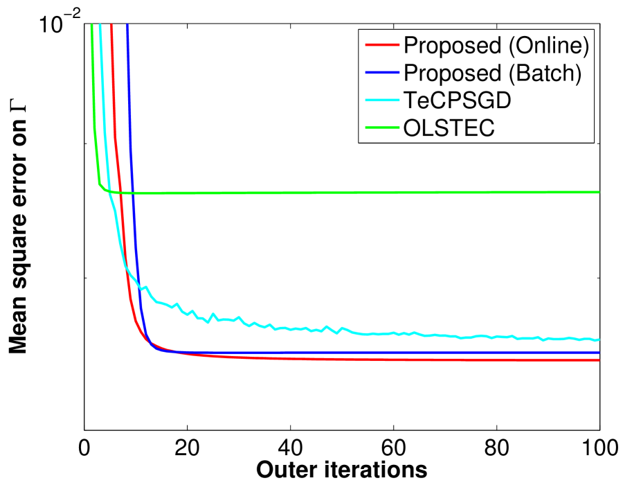
Case O: online instances. We compare the proposed stochastic gradient descent algorithm with its batch counterpart gradient descent algorithm and with TeCPSGD Mardani et al. (2015) and OLSTEC Kasai (2016). As the implementations of TeCPSGD and OLSTEC are computationally more intensive than ours, our plots only show test MSE against the number of outer iterations, i.e., the number of the passes through the data.
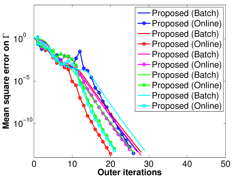
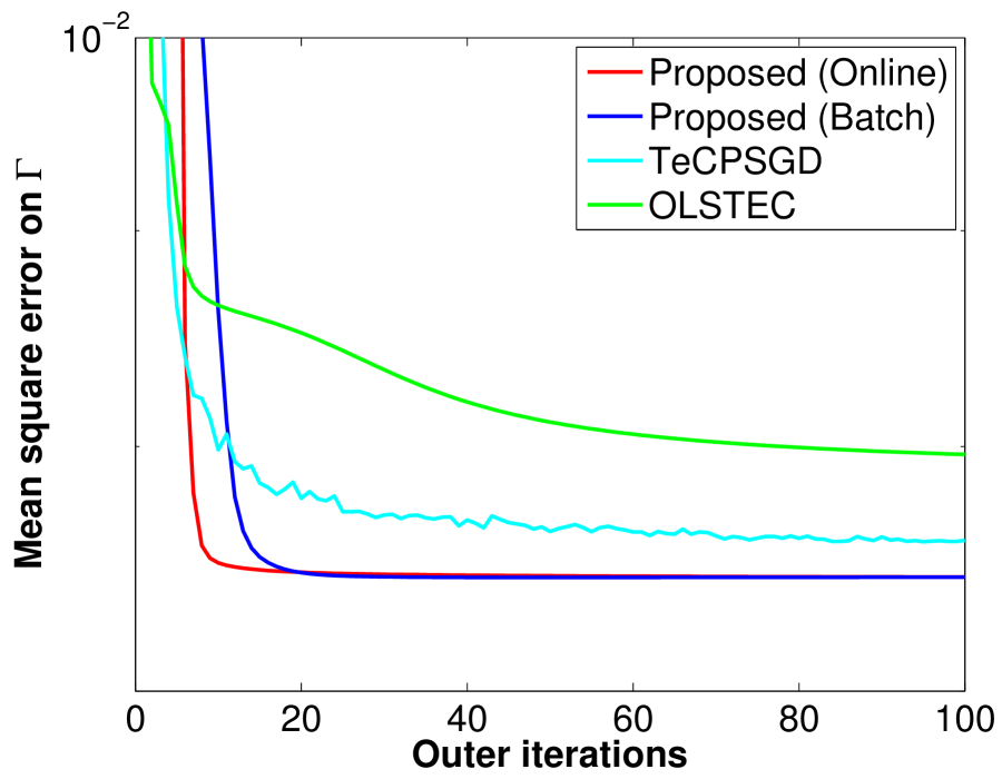
Figure 3(a) shows comparisons on a synthetic instance of tensor size with rank . is selected from the step-size list in the pre-training phase. entries are randomly observed. The pre-training uses frontal slices of all the slices. The maximum number of outer loops is set to . Figure 3(a) shows five different runs, where the online algorithm has the same asymptotic convergence behavior as the batch counterpart on a test dataset . Figure 3(b) shows comparisons on the Airport Hall surveillance video sequence dataset333http://perception.i2r.a-star.edu.sg/bk_model/bk_index.html of size with frames. is selected from and frontal slices are selected for pre-training. of the entries are observed. In Figure 3(b), both the proposed online and batch algorithms achieve lower test errors than TeCPSGD and OLSTEC.
6 Conclusion
We have proposed preconditioned batch (conjugate gradient) and online (stochastic gradient descent) algorithms for the tensor completion problem. The algorithms stem from the Riemannian preconditioning approach that exploits the fundamental structures of symmetry (due to non-uniqueness of Tucker decomposition) and least-squares of the cost function. A novel Riemannian metric (inner product) is proposed that enables to use the versatile Riemannian optimization framework. Numerical comparisons suggest that our proposed algorithms have a superior performance on different benchmarks.
Acknowledgments
We thank Rodolphe Sepulchre, Paul Van Dooren, and Nicolas Boumal for useful discussions on the paper. This paper presents research results of the Belgian Network DYSCO (Dynamical Systems, Control, and Optimization), funded by the Interuniversity Attraction Poles Programme, initiated by the Belgian State, Science Policy Office. The scientific responsibility rests with its authors. Hiroyuki Kasai is (partly) supported by the Ministry of Internal Affairs and Communications, Japan, as the SCOPE Project (150201002). This work was initiated while Bamdev Mishra was with the Department of Electrical Engineering and Computer Science, University of Liège, 4000 Liège, Belgium and was visiting the Department of Engineering (Control Group), University of Cambridge, Cambridge, UK. He was supported as a research fellow (aspirant) of the Belgian National Fund for Scientific Research (FNRS).
References
- Absil et al. [2008] Absil, P.-A., Mahony, R., and Sepulchre, R. Optimization Algorithms on Matrix Manifolds. Princeton University Press, 2008.
- Bonnabel [2013] Bonnabel, S. Stochastic gradient descent on Riemannian manifolds. IEEE Trans. Autom. Control, 58(9):2217–2229, 2013.
- Bottou [2012] Bottou, L. Stochastic gradient descent tricks. Neural Networks: Tricks of the Trade (2nd ed.), pp. 421–436, 2012.
- Boumal & Absil [2015] Boumal, N. and Absil, P.-A. Low-rank matrix completion via preconditioned optimization on the Grassmann manifold. Linear Algebra Appl., 475:200–239, 2015.
- Boumal et al. [2014] Boumal, N., Mishra, B., Absil, P.-A., and Sepulchre, R. Manopt: a Matlab toolbox for optimization on manifolds. J. Mach. Learn. Res., 15(1):1455–1459, 2014.
- Candès & Recht [2009] Candès, E. J. and Recht, B. Exact matrix completion via convex optimization. Found. Comput. Math., 9(6):717–772, 2009.
- Edelman et al. [1998] Edelman, A., Arias, T.A., and Smith, S.T. The geometry of algorithms with orthogonality constraints. SIAM J. Matrix Anal. Appl., 20(2):303–353, 1998.
- Filipović & Jukić [2013] Filipović, M. and Jukić, A. Tucker factorization with missing data with application to low-n-rank tensor completion. Multidim. Syst. Sign. P., 2013. Doi: 10.1007/s11045-013-0269-9.
- Foster et al. [2007] Foster, D. H., Nascimento, S. M. C., and Amano, K. Information limits on neural identification of colored surfaces in natural scenes. Visual Neurosci., 21(3):331–336, 2007.
- Kasai [2016] Kasai, H. Online low-rank tensor subspace tracking from incomplete data by CP decomposition using recursive least squares. In IEEE ICASSP, 2016.
- Kasai & Mishra [2015] Kasai, Hiroyuki and Mishra, Bamdev. Riemannian preconditioning for tensor completion. Technical report, arXiv preprint arXiv:1506.02159, 2015.
- Kolda & Bader [2009] Kolda, T. G. and Bader, B. W. Tensor decompositions and applications. SIAM Rev., 51(3):455–500, 2009.
- Kressner et al. [2014] Kressner, D., Steinlechner, M., and Vandereycken, B. Low-rank tensor completion by Riemannian optimization. BIT Numer. Math., 54(2):447–468, 2014.
- Lee [2003] Lee, J. M. Introduction to smooth manifolds, volume 218 of Graduate Texts in Mathematics. Springer-Verlag, New York, second edition, 2003.
- Liu et al. [2013] Liu, J., Musialski, P., Wonka, P., and Ye, J. Tensor completion for estimating missing values in visual data. IEEE Trans. Pattern Anal. Mach. Intell., 35(1):208–220, 2013.
- Mardani et al. [2015] Mardani, M., Mateos, G., and Giannakis, G.B. Subspace learning and imputation for streaming big data matrices and tensors. IEEE Trans. Signal Process., 63(10):266 –2677, 2015.
- Mishra & Sepulchre [2014] Mishra, B. and Sepulchre, R. R3MC: A Riemannian three-factor algorithm for low-rank matrix completion. In IEEE CDC, pp. 1137–1142, 2014.
- Mishra & Sepulchre [2016] Mishra, B. and Sepulchre, R. Riemannian preconditioning. SIAM J. Optim., 26(1):635–660, 2016.
- Ngo & Saad [2012] Ngo, T. and Saad, Y. Scaled gradients on Grassmann manifolds for matrix completion. In NIPS, pp. 1421–1429, 2012.
- Nocedal & Wright [2006] Nocedal, J. and Wright, S. J. Numerical Optimization, volume Second Edition. Springer, 2006.
- Ring & Wirth [2012] Ring, W. and Wirth, B. Optimization methods on Riemannian manifolds and their application to shape space. SIAM J. Optim., 22(2):596–627, 2012.
- Sato & Iwai [2015] Sato, H. and Iwai, T. A new, globally convergent Riemannian conjugate gradient method. Optimization, 64(4):1011–1031, 2015.
- Signoretto et al. [2011] Signoretto, M., Plas, R. V. d., Moor, B. D., and Suykens, J. A. K. Tensor versus matrix completion: A comparison with application to spectral data. IEEE Signal Process. Lett., 18(7):403–406, 2011.
- Signoretto et al. [2014] Signoretto, M., Dinh, Q. T., Lathauwer, L. D., and Suykens, J. A. K. Learning with tensors: a framework based on convex optimization and spectral regularization. Mach. Learn., 94(3):303–351, 2014.
- Tomioka et al. [2011] Tomioka, R., Hayashi, K., and Kashima, H. Estimation of low-rank tensors via convex optimization. Technical report, arXiv preprint arXiv:1010.0789, 2011.
- Vandereycken [2013] Vandereycken, B. Low-rank matrix completion by Riemannian optimization. SIAM J. Optim., 23(2):1214–1236, 2013.
- Wen et al. [2012] Wen, Z., Yin, W., and Zhang, Y. Solving a low-rank factorization model for matrix completion by a nonlinear successive over-relaxation. Math Program. Comput., 4(4):333–361, 2012.
Appendix A Proof and derivation of manifold-related ingredients
The concrete computations of the optimization-related ingredients presented in the paper are discussed below.
The total space is . Each element has the matrix representation . Invariance of Tucker decomposition under the transformation for all , the set of orthogonal matrices of size of results in equivalence classes of the form .
A.1 Tangent space characterization and the Riemannian metric
The tangent space, , at given by in the total space is the product space of the tangent spaces of the individual manifolds. From [1], the tangent space has the matrix characterization
| (A.1) |
The proposed metric is
| (A.2) |
where are tangent vectors with matrix characterizations and , respectively and is the Euclidean inner product.
A.2 Characterization of the normal space
Given a vector in , its projection onto the tangent space is obtained by extracting the component normal, in the metric sense, to the tangent space. This section describes the characterization of the normal space, .
Let , and . Since is orthogonal to , i.e., , the conditions
| (A.3) |
must hold for all in the tangent space. Additionally from [1], has the characterization
| (A.4) |
where is any skew-symmetric matrix, K is a any matrix of size , and is any that is orthogonal complement of . Let and let is defined as
| (A.5) |
without loss of generality, where and are to be characterized from (A.3) and (A.4). A few standard computations show that A has to be symmetric and . Consequently, , where . Equivalently, for a symmetric matrix . Finally, the normal space has the characterization
| (A.6) |
A.3 Characterization of the vertical space
The horizontal space projector of a tangent vector is obtained by removing the component along the vertical direction. This section shows the matrix characterization of the vertical space .
is the defined as the linearization of the equivalence class at . Equivalently, is the linearization of along at the identity element for . From the characterization of linearization of an orthogonal matrix [1], we have the characterization for the vertical space as
| (A.7) |
A.4 Characterization of the horizontal space
The characterization of the horizontal space is derived from its orthogonal relationship with the vertical space .
Let , and . Since must be orthogonal to , which is equivalent to in (A.2), the characterization for is derived from (A.2) and (A.7).
where is the mode- unfolding of . Since above should be zero for all skew-matrices , must satisfy
| (A.8) |
A.5 Proof of Proposition 1
We first introduce the following lemma:
Lemma 1.
Let and be a tangent vector to the quotient manifold at . The horizontal lifts of at and are related for as follows,
| (A.9) |
Proof.
Let be an arbitrary smooth function, and define
where is the mapping defined by .
Consider the mapping
where . Since for all , we have
By taking the differential of both sides,
| (A.10) |
By noting the definition of , i.e., , the right side of (A.10) is
where the chain rule is applied to the first equality.
Moreover, from the directional derivatives of the mapping , the bracket of the left side of (A.10) is obtained as
Therefore, (A.10) yields
| (A.11) |
where we address the equivalence class . The left side of (A.11) is further transformed by the chain rule as
| (A.12) |
By comparing the right sides of (A.11) and (A.12), since this equality holds for any smooth function , it implies that
| (A.13) |
Finally, we check whether is an element of
.
Addressing that the mode- unfolding of is , plugging into in (A.8) yields
| (A.14) |
Since is a symmetric matrix, the obtained result is also symmetric. Therefore, is a horizontal vector at . This implies that is the horizontal lift of at , and the proof is completed. ∎
Now, the proof of Proposition 1 is given below using the result (A.9) in Lemma 1.
A.6 Proof of Proposition 2 (derivation of the tangent space projector)
Proof.
The tangent space projector is obtained by extracting the component normal to in the ambient space. The normal space has the matrix characterization shown in (A.6). The operator has the expression
| (A.15) |
From the definition of the tangent space in (A.1), should satisfy
Multiplying from the right and left sides results in
Finally, we obtain the Lyapunov equation as
| (A.16) |
that are solved efficiently with the Matlab’s lyap routine.
∎
A.7 Proof of Proposition 3 (derivation of the horizontal space projector)
Proof.
We consider the projection of a tangent vector into a vector . This is achieved by subtracting the component in the vertical space in (A.7) as
As a result, the horizontal operator has the expression
| (A.18) |
where and is a skew-symmetric matrix of size . The skew-matrices for that are identified based on the conditions (A.8).
It should be noted that the tensor in (A.7) has the following equivalent unfoldings.
Plugging and into (A.8) and using the relation results in
which should be a symmetric matrix due to (A.8), i.e., .
Subsequently,
which is equivalent to
Here extracts the skew-symmetric part of a square matrix, i.e., .
Finally, we obtain the coupled Lyapunov equations
| (A.21) |
that are solved efficiently with the Matlab’s pcg routine that is combined with a specific preconditioner resulting from the Gauss-Seidel approximation of (A.21).
∎
A.8 Proof of Proposition 4 (derivation of the Riemannian gradient formula)
Proof.
Let and be an auxiliary sparse tensor variable that is interpreted as the Euclidean gradient of in .
The partial derivatives of are
where is mode- unfolding of and
Due to the specific scaled metric (A.2), the partial derivatives of are further scaled by , denoted as (after scaling), i.e.,
Consequently, from the relationship that horizontal lift of is equal to , we obtain that, using (A.15),
From the requirements in (A.16) for a vector to be in the tangent space, we have the following relationship for mode-.
where .
Subsequently,
Finally, for are obtained by solving the Lyapunov equations
where extracts the symmetric part of a square matrix, i.e., . The above Lyapunov equations are solved efficiently with the Matlab’s lyap routine.
∎
Appendix B Additional numerical comparisons
In addition to the representative numerical comparisons in the paper, we show additional numerical experiments spanning synthetic and real-world datasets.
Experiments on synthetic datasets:
Case S1: comparison with the Euclidean metric. We first show the benefit of the proposed metric (A.2) over the conventional choice of the Euclidean metric that exploits the product structure of and symmetry. We compare steepest descent algorithms with Armijo backtracking linesearch for both the metric choices. Figure A.1 shows that the algorithm with the metric (A.2) gives a superior performance in test error than that of the conventional metric choice.
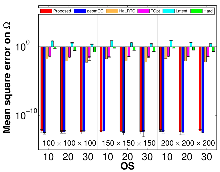
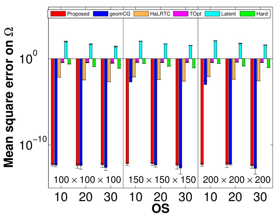
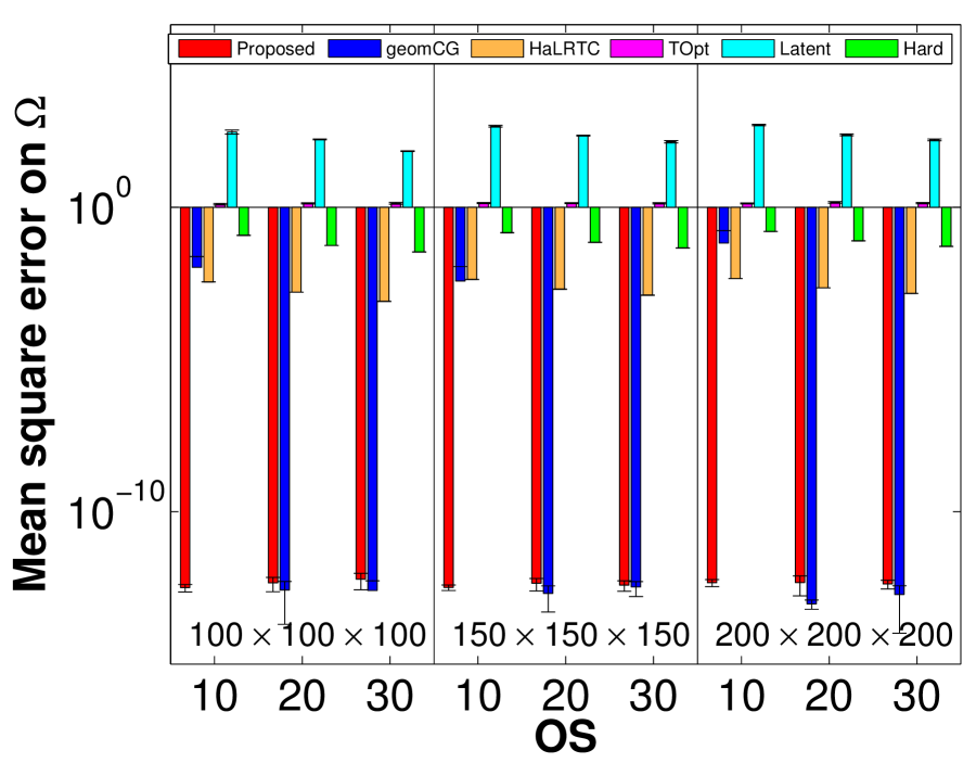
Case S2: small-scale instances. We consider tensors of size , , and and ranks , , and . OS is . Figures A.2(a)-(c) and Figures A.3(a)-(c) show the convergence behavior of different algorithms on a train set and on a test set , where Figures A.3(b) is identical to the figure in the manuscript paper. Figures A.2(d)-(f) and A.3(d)-(f) show the mean square error on and on each algorithm. Furthermore, Figure A.2(g)-(i) and Figure A.3(g)-(i) show the mean square error on and when OS is in all the five runs. From Figures A.2 and Figures A.3, our proposed algorithm is consistently competitive or faster than geomCG, HalRTC, and TOpt. In addition, the mean square errors on a train set and a test set are consistently competitive or lower than those of geomCG and HalRTC, especially for lower sampling ratios, e.g, for OS .
Case S3: large-scale instances. We consider large-scale tensors of size , , and and ranks r= and . OS is . We compare our proposed algorithm to geomCG. Figure A.4 and Figure A.5 show the convergence behavior of the algorithms. The proposed algorithm outperforms geomCG in all the cases.
Case S4: influence of low sampling. We look into problem instances which result from scarcely sampled data. The test requires completing a tensor of size and rank r=. Figure A.9 and Figure A.9 show the convergence behavior when OS is . The case of is particularly interesting. In this case, while the mean square errors on and increase for geomCG, the proposed algorithm stably decreases the error in all the five runs.
Case S5: influence of ill-conditioning and low sampling. We consider the problem instance of Case S4 with . Additionally, for generating the instance, we impose a diagonal core with exponentially decaying positive values of condition numbers (CN) , , and . Figure A.9 shows that the proposed algorithm outperforms geomCG for all the considered CN values on a train set .
Case S6: influence of noise. We evaluate the convergence properties of algorithms under the presence of noise The tensor size and rank are same as in Case S4 and OS is . Figure A.9 shows that the train error on a train set for each is almost identical to the , but our proposed algorithm converges faster than geomCG.
Case S7: rectangular instances. We consider instances where dimensions and ranks along certain modes are different than others. Two cases are considered. Case (7.a) considers tensors size , , and and rank . Case (7.b) considers a tensor of size with ranks , , and . Figures A.11(a)-(c) and Figures A.11(a)-(c) show that the convergence behavior of our proposed algorithm is superior to that of geomCG on and , respectively. Our proposed algorithm also outperforms geomCG for the asymmetric rank cases as shown in Figure A.11(d)-(f) and Figure A.11(d)-(f).
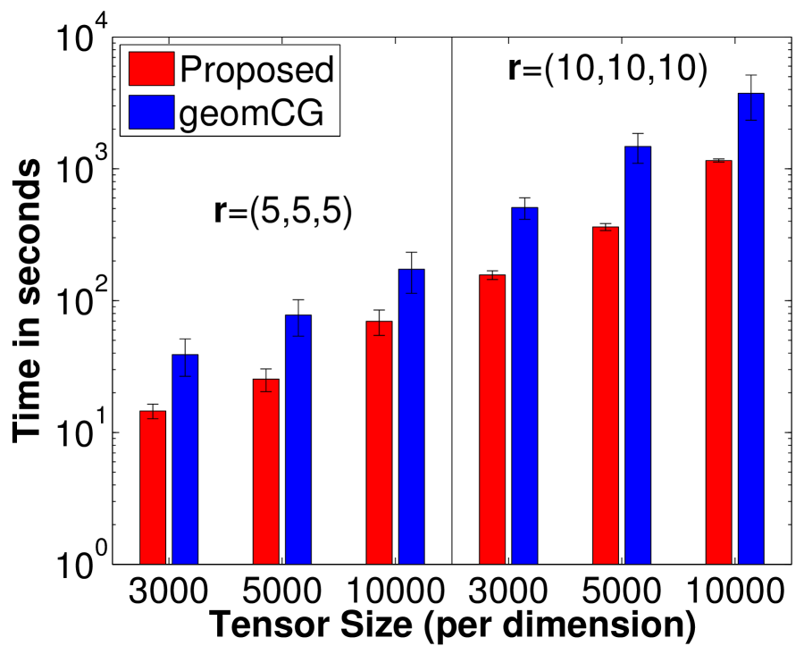
Case S8: medium-scale instances. We additionally consider medium-scale tensors of size , , and and ranks , and . OS is . Our proposed algorithm and geomCG are only compared as the other algorithms cannot handle these scales efficiently. Figures A.13(a)-(c) and A.13(a)-(c) show the convergence behavior on and , respectively. Figures A.13(d)-(f) and Figures A.13(d)-(f) also show the mean square error on and of rank in all the five runs. The proposed algorithm performs better than geomCG in all the cases.
Experiments on real-world datasets:
Case R1: hyperspectral image. We also show the performance of our algorithm on the hyperspectral image “Ribeira”. We show the mean square error on and when OS is in Figure A.14 and Figure A.15, where Figure A.15(a) is identical to the figure in the manuscript paper. Our proposed algorithm gives lower test errors than those obtained by the other algorithms. We also show the image recovery results. Figures A.16 and A.17 show the reconstructed images when OS is , respectively. From these figures, we find that the proposed algorithm shows a good performance, especially for the lower sampling ratio.
Case R2: MovieLens-10M. Figure A.18 and Figure A.19 show the convergence plots for all the five runs of ranks , , and on and , respectively. These figures show the superior performance of our proposed algorithm.
Experiments for online algorithms:
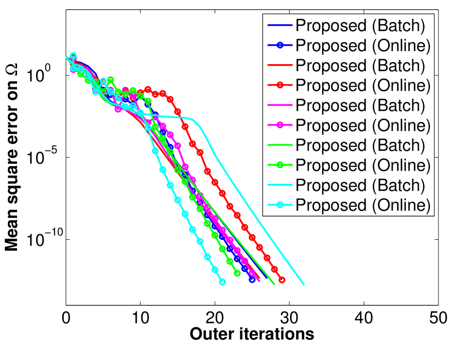
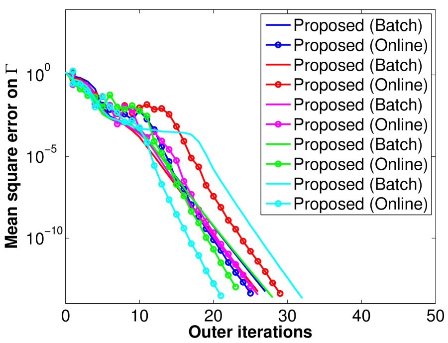
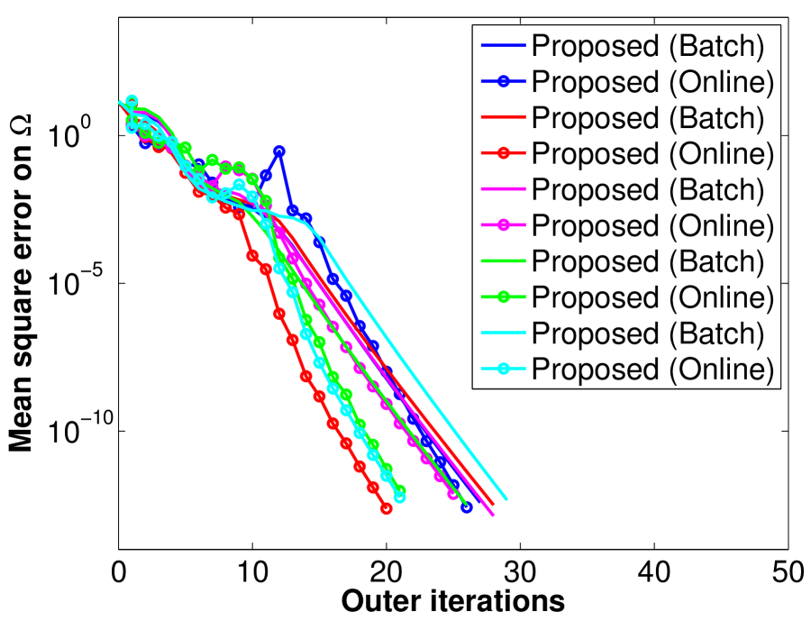
Case O: online instances. Figure A.21 and A.21 show the convergence plots for all the five runs on tensors of ranks , and with rank on and , respectively. These figures show that the proposed stochastic gradient descent algorithm gives similar or faster convergence than the proposed batch gradient descent algorithm.
Figure A.23 and A.23 show the convergence speed comparisons in the train error and the test error of the proposed online and batch algorithms with TeCPSGD and OLSTEC with rank on the real-world video sequence Airport Hall dataset. These figures show that the proposed stochastic gradient descent algorithm gives similar or faster convergence than the proposed batch algorithm. In addition, Table A.1 shows that the final train and test MSEs show the superior performance of the proposed algorithms.
 (a) r = ().
 (b) r = ().
 (c) r = ().
|
 (d) r = ().
 (e) r = ().
 (f) r = ().
|
 (g) , OS = ,
r = (). 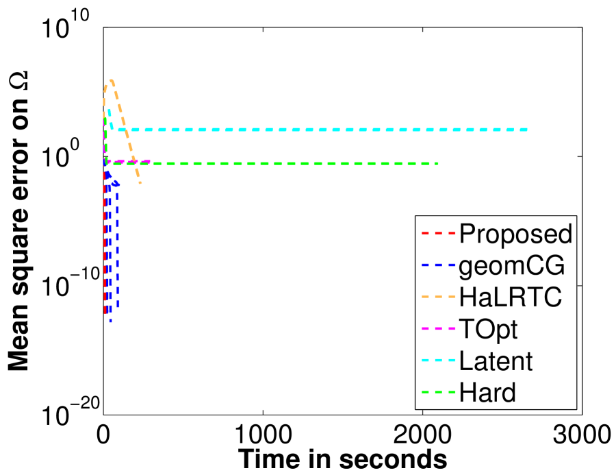 (h) , OS = ,
r = (). 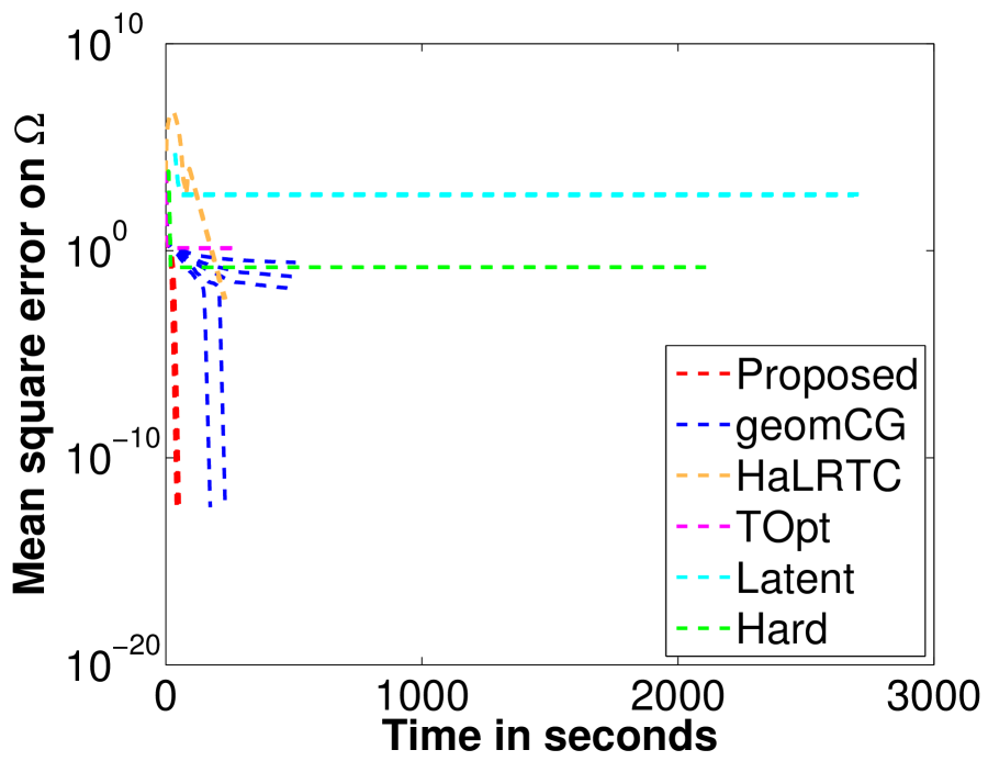 (i) , OS = ,
r = (). |
 (a) r = ().
 (b) r = ().
 (c) r = ().
|
 (d) r = ().
 (e) r = ().
 (f) r = ().
|
 (g) , OS = ,
r = (). 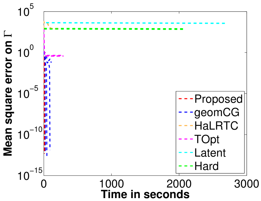 (h) , OS = ,
r = (). 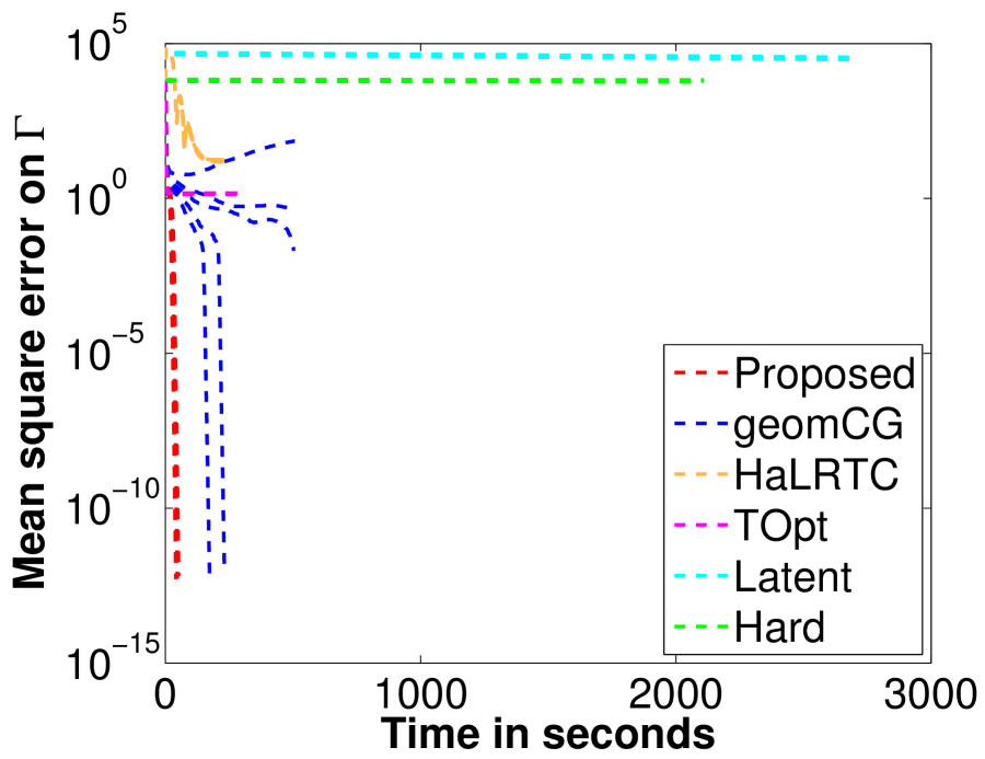 (i) , OS = ,
r = (). |
 (a) ,
(a) ,
r = ().  (b) ,
(b) ,
r = (). 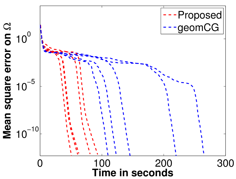 (c) ,
(c) ,
r = (). |
 (d) ,
(d) ,
r = (). 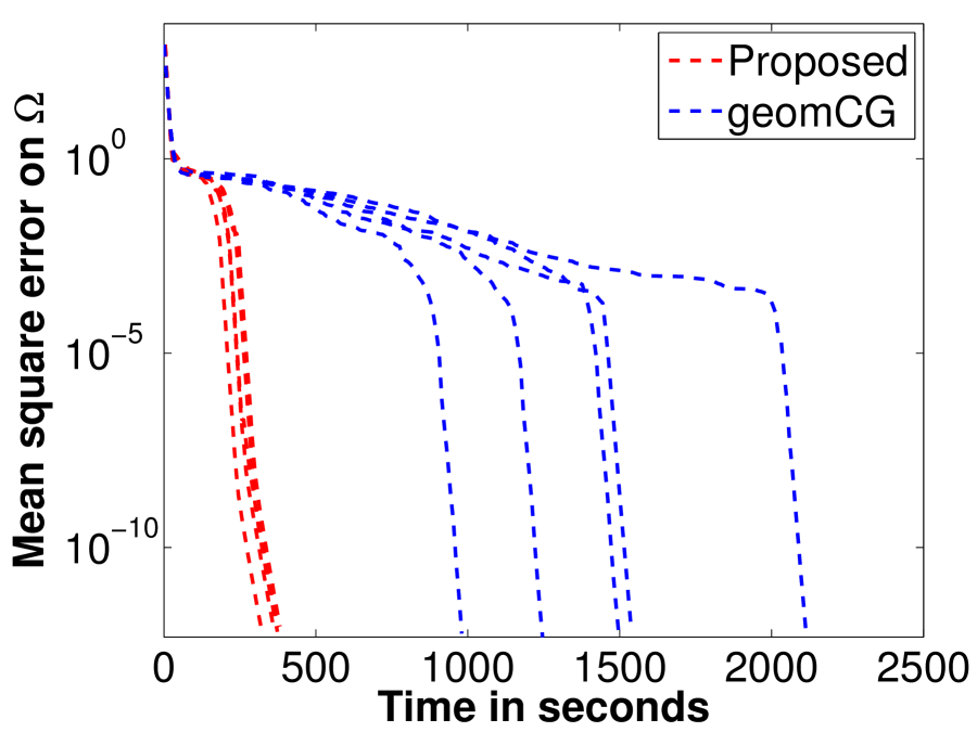 (e) ,
(e) ,
r = ().  (f) ,
(f) ,
r = (). |
 (a) ,
(a) ,
r = (). 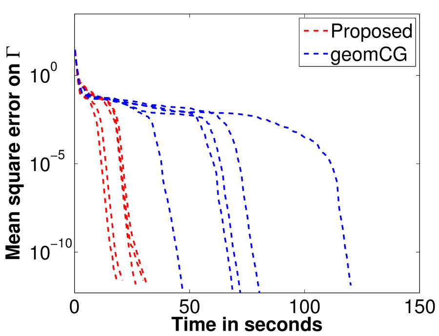 (b) ,
(b) ,
r = ().  (c) ,
(c) ,
r = (). |
 (d) ,
(d) ,
r = (). 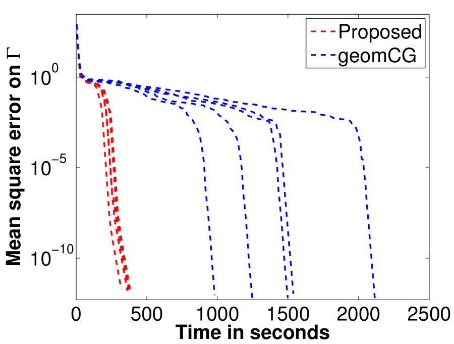 (e) ,
(e) ,
r = (). 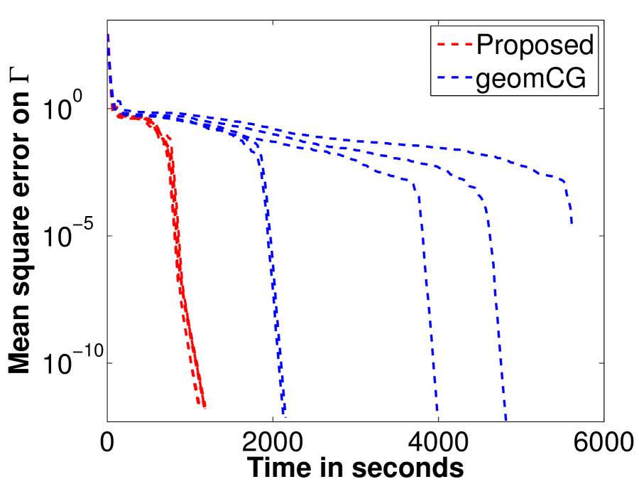 (f) ,
(f) ,
r = (). |
 (a) OS = .
 (b) OS = .
 (c) OS = .
|
 (a) OS = .
 (b) OS = .
 (c) OS = .
|
 (a) ,
(a) ,
r = (). 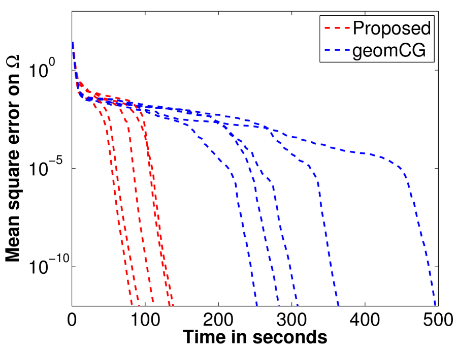 (b) ,
(b) ,
r = (). 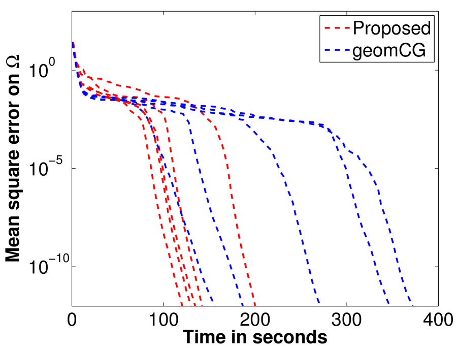 (c) ,
(c) ,
r = (). |
 (d) r = (),
.  (e) r = (),
.  (f) r = (),
. |
 (a) ,
(a) ,
r = (). 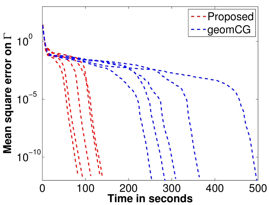 (b) ,
(b) ,
r = (). 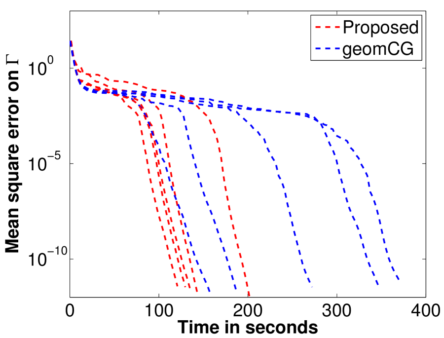 (c) ,
(c) ,
r = (). |
 (d) r = (),
.  (e) r = (),
.  (f) r = (),
. |
 (a) r = ().
 (b) r = ().
 (c) r = ().
|
 (d) ,
(d) ,
r = (). 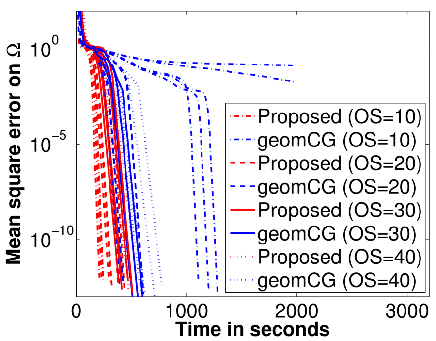 (e) ,
(e) ,
r = (). 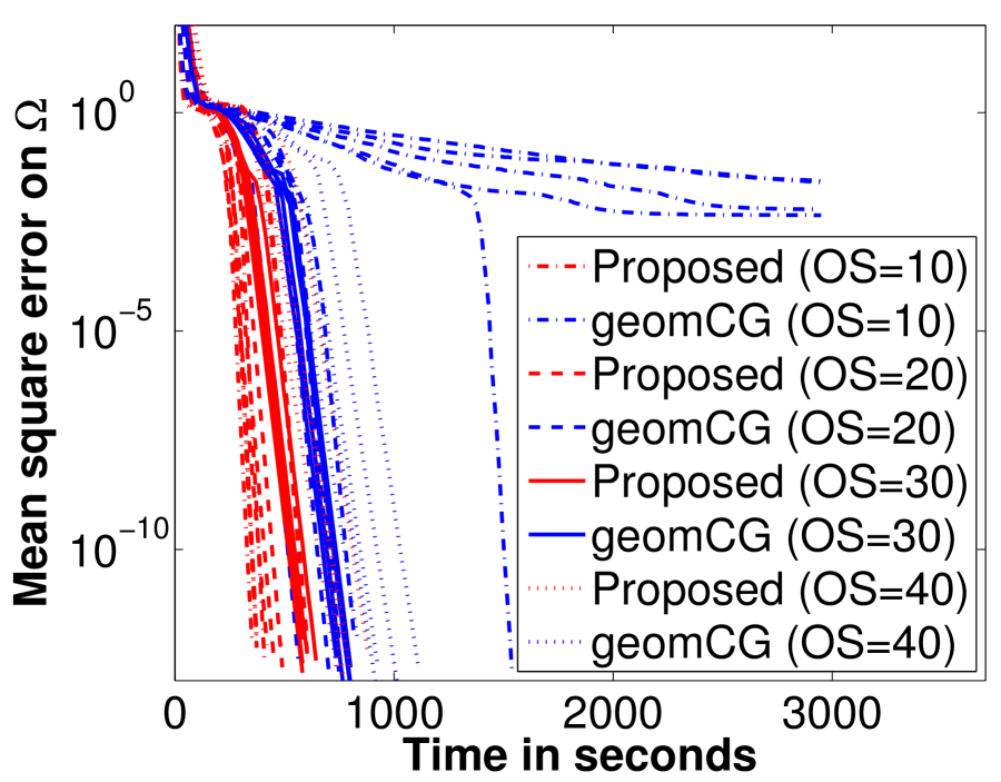 (f) ,
(f) ,
r = (). |
 (a) r = ().
 (b) r = ().
 (c) r = ().
|
 (d) ,
(d) ,
r = (). 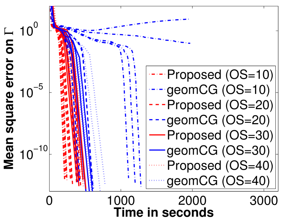 (e) ,
(e) ,
r = (). 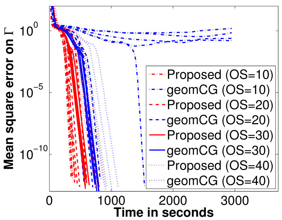 (f) ,
(f) ,
r = (). |
 (a) OS = .
 (b) OS = .
|
 (a) OS = .
 (b) OS = .
|
 (a) Original.
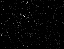 (b) Sampled (% observed).
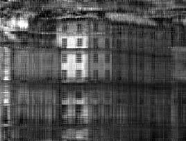 (c) Proposed.
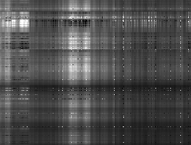 (d) geomCG.
|
 (e) HaLRTC.
 (f) TOpt.
 (g) Latent.
 (h) Hard.
|
(a) Original.
 (b) Sampled ( observed).
 (c) Proposed.
 (d) geomCG.
|
 (e) HaLRTC.
 (f) TOpt.
 (g) Latent.
 (h) Hard.
|
 (a) r = ().
 (b) r = ().
|
 (c) r = ().
 (d) r = ().
|
 (a) r = ().
 (b) r = ().
|
 (c) r = ().
 (d) r = ().
|
 (a) Mean square error on (train error).
 (b) Mean square error on (test error).
|
 (a) Mean square error on (train error).
 (b) Mean square error on (test error).
|
| Error type | Algorithm | run 1 | run 2 | run 3 | run 4 | run 5 |
|---|---|---|---|---|---|---|
| Training error | Proposed (Online) | 7.210000 | 7.211718 | 7.205027 | 7.255203 | 7.230000 |
| on | Proposed (Batch) | 7.215763 | 7.211496 | 7.208463 | 7.282901 | 7.218042 |
| TeCPSGD | 7.335320 | 7.389269 | 7.364065 | 7.393318 | 7.390530 | |
| OLSTEC | 7.922385 | 7.653096 | 8.150799 | 8.248936 | 7.753596 | |
| Test error | Proposed (Online) | 7.462097 | 7.440332 | 7.452799 | 7.443505 | 7.450065 |
| on | Proposed (Batch) | 7.471942 | 7.440508 | 7.446072 | 7.492786 | 7.218042 |
| TeCPSGD | 7.592109 | 7.601955 | 7.600740 | 7.579759 | 7.600621 | |
| OLSTEC | 8.205765 | 7.840107 | 8.599819 | 8.625715 | 7.965405 |
 (a) Run 1.
 (b) Run 2.
 (c) Run 3.
|
 (d) Run 4.
 (e) Run 5.
|
 (a) Run 1.
 (b) Run 2.
 (c) Run 3.
|
 (d) Run 4.
 (e) Run 5.
|